Last updated: 2026-02-17
Checks:
Knit directory: jovial-shockley/
This reproducible R Markdown
analysis was created with workflowr (version
1.7.1). The Checks tab describes the reproducibility checks
that were applied when the results were created. The Past
versions tab lists the development history.
Great! Since the R Markdown file has been committed to the Git
repository, you know the exact version of the code that produced these
results.
Great job! The global environment was empty. Objects defined in the
global environment can affect the analysis in your R Markdown file in
unknown ways. For reproduciblity it’s best to always run the code in an
empty environment.
The command set.seed(20260127) was run prior to running
the code in the R Markdown file. Setting a seed ensures that any results
that rely on randomness, e.g. subsampling or permutations, are
reproducible.
Nice! There were no cached chunks for this analysis, so you can be
confident that you successfully produced the results during this
run.
Great job! Using relative paths to the files within your workflowr
project makes it easier to run your code on other machines.
Great! You are using Git for version control. Tracking code development
and connecting the code version to the results is critical for
reproducibility.
The results in this page were generated with repository version
c592bd3 .
See the Past versions tab to see a history of the changes made
to the R Markdown and HTML files.
Note that you need to be careful to ensure that all relevant files for
the analysis have been committed to Git prior to generating the results
(you can use wflow_publish or
wflow_git_commit). workflowr only checks the R Markdown
file, but you know if there are other scripts or data files that it
depends on. Below is the status of the Git repository when the results
were generated:
Ignored files:
    Ignored:    .claude/
    Ignored:    renv/library/
    Ignored:    renv/staging/

Untracked files:
    Untracked:  Data/laconia_messinia_cups_skulls.csv
    Untracked:  Data/period_dictionary.csv
    Untracked:  Data/tomb_type_dictionary.csv

Unstaged changes:
    Deleted:    data/laconia_messinia_cups_skulls - Sheet2.csv
Note that any generated files, e.g. HTML, png, CSS, etc., are not
included in this status report because it is ok for generated content to
have uncommitted changes.
These are the previous versions of the repository in which changes were
made to the R Markdown
(analysis/cups_and_skulls_analysis.Rmd) and HTML
(docs/cups_and_skulls_analysis.html) files. If you’ve
configured a remote Git repository (see ?wflow_git_remote),
click on the hyperlinks in the table below to view the files as they
were in that past version.
File
Version
Author
Date
Message
Rmd
c592bd3
tinalasisi
2026-02-17
Add data dictionary worksheet and chamber space analysis
Introduction
This analysis examines the relationship between drinking vessels and
human skeletal remains in Laconian and Messinian tholos and chamber
tombs. The data focuses on grave contexts where drinking vessels are
recorded alongside information about primary and secondary burials.
Load Libraries
library(readr)
library(dplyr)
library(ggplot2)
library(tidyr)
library(stringr)
library(janitor)
library(knitr)
Load Data
# Load the CSV data
data_path <- here::here("data", "laconia_messinia_cups_skulls.csv")
cups_skulls <- read_csv(data_path)
Rows: 296 Columns: 14
── Column specification ────────────────────────────────────────────────────────
Delimiter: ","
chr (11): Grave ID, site, type, period, secondary, primary, dimensions, orie...
dbl (3): drinking vessel number, skulls number, area of chamber estimated
ℹ Use `spec()` to retrieve the full column specification for this data.
ℹ Specify the column types or set `show_col_types = FALSE` to quiet this message.# Display dimensions
cat("Dataset dimensions:", nrow(cups_skulls), "graves ×", ncol(cups_skulls), "columns\n")Dataset dimensions: 296 graves × 14 columns# Show column names
glimpse(cups_skulls)Rows: 296
Columns: 14
$ `Grave ID` <chr> "vapheio_tholos", "arkynes_tholos_A", "ark…
$ site <chr> "Vapheio", "Arkynes", "Arkynes", "Arkynes"…
$ type <chr> "tholos", "tholos", "tholos", "tholos", "t…
$ period <chr> "LHIIA-LHIIIA1", "LHIIIA- LHIIIB", "LHIII"…
$ secondary <chr> "absent", "absent", "absent", "present", "…
$ primary <chr> "absent", "absent", "present", "absent", "…
$ dimensions <chr> "83.28m^2. dromos: L 29.8m x w3.18-3.45, s…
$ orientation <chr> "NE-SW", "SE-NW", NA, NA, "E-W", "N-S", "W…
$ `drinking vessel` <chr> "yes", "no", "no", "no", "no", "no", "no",…
$ remains <chr> "yes", "yes", "yes", "yes", "yes", "no", "…
$ `drinking vessel number` <dbl> 6, NA, NA, NA, NA, NA, NA, 4, NA, NA, 5, N…
$ `skulls number` <dbl> NA, NA, NA, NA, NA, NA, NA, NA, NA, NA, NA…
$ `area of chamber estimated` <dbl> 84.130, 17.350, NA, 28.274, 7.793, NA, 18.…
$ region <chr> "laconia", "laconia", "laconia", "laconia"…
Data Cleaning
cups_skulls_clean <- cups_skulls %>%
  # Clean column names
  janitor::clean_names() %>%

  # Trim whitespace from character columns
  mutate(across(where(is.character), str_trim)) %>%

  # Standardize yes/no values in drinking vessel column
  mutate(
    has_drinking_vessel = case_when(
      tolower(drinking_vessel) == "yes" ~ TRUE,
      tolower(drinking_vessel) == "no" ~ FALSE,
      TRUE ~ NA
    ),
    has_remains = case_when(
      tolower(remains) == "yes" ~ TRUE,
      tolower(remains) == "no" ~ FALSE,
      TRUE ~ NA
    ),
    primary_burial = case_when(
      tolower(primary) == "present" ~ TRUE,
      tolower(primary) == "absent" ~ FALSE,
      TRUE ~ NA
    ),
    secondary_burial = case_when(
      tolower(secondary) == "present" ~ TRUE,
      tolower(secondary) == "absent" ~ FALSE,
      TRUE ~ NA
    )
  ) %>%

  # Create burial category
  mutate(
    burial_category = case_when(
      primary_burial & secondary_burial ~ "Both Primary & Secondary",
      primary_burial & !secondary_burial ~ "Primary Only",
      !primary_burial & secondary_burial ~ "Secondary Only",
      TRUE ~ "Unknown/Not Recorded"
    )
  ) %>%

  # Simplify grave type
  mutate(
    grave_type_simple = case_when(
      str_detect(tolower(type), "tholos") ~ "Tholos",
      str_detect(tolower(type), "chamber") ~ "Chamber Tomb",
      str_detect(tolower(type), "cist") ~ "Cist Grave",
      str_detect(tolower(type), "pit") ~ "Pit Grave",
      str_detect(tolower(type), "dromos") ~ "Dromos Only",
      TRUE ~ "Other"
    )
  )

# Show cleaned data structure
glimpse(cups_skulls_clean)
Rows: 296
Columns: 20
$ grave_id <chr> "vapheio_tholos", "arkynes_tholos_A", "arkyn…
$ site <chr> "Vapheio", "Arkynes", "Arkynes", "Arkynes", …
$ type <chr> "tholos", "tholos", "tholos", "tholos", "tho…
$ period <chr> "LHIIA-LHIIIA1", "LHIIIA- LHIIIB", "LHIII", …
$ secondary <chr> "absent", "absent", "absent", "present", "pr…
$ primary <chr> "absent", "absent", "present", "absent", "pr…
$ dimensions <chr> "83.28m^2. dromos: L 29.8m x w3.18-3.45, sto…
$ orientation <chr> "NE-SW", "SE-NW", NA, NA, "E-W", "N-S", "W-E…
$ drinking_vessel <chr> "yes", "no", "no", "no", "no", "no", "no", "…
$ remains <chr> "yes", "yes", "yes", "yes", "yes", "no", "no…
$ drinking_vessel_number <dbl> 6, NA, NA, NA, NA, NA, NA, 4, NA, NA, 5, NA,…
$ skulls_number <dbl> NA, NA, NA, NA, NA, NA, NA, NA, NA, NA, NA, …
$ area_of_chamber_estimated <dbl> 84.130, 17.350, NA, 28.274, 7.793, NA, 18.32…
$ region <chr> "laconia", "laconia", "laconia", "laconia", …
$ has_drinking_vessel <lgl> TRUE, FALSE, FALSE, FALSE, FALSE, FALSE, FAL…
$ has_remains <lgl> TRUE, TRUE, TRUE, TRUE, TRUE, FALSE, FALSE, …
$ primary_burial <lgl> FALSE, FALSE, TRUE, FALSE, TRUE, FALSE, FALS…
$ secondary_burial <lgl> FALSE, FALSE, FALSE, TRUE, TRUE, FALSE, FALS…
$ burial_category <chr> "Unknown/Not Recorded", "Unknown/Not Recorde…
$ grave_type_simple <chr> "Tholos", "Tholos", "Tholos", "Tholos", "Tho…
Data Overview
Basic Statistics
cat("=== Dataset Summary ===\n\n")=== Dataset Summary ===cat("Total graves:", nrow(cups_skulls_clean), "\n")Total graves: 296 cat("Graves with drinking vessels recorded:", sum(cups_skulls_clean$has_drinking_vessel == TRUE, na.rm = TRUE), "\n")Graves with drinking vessels recorded: 80 cat("Graves with human remains:", sum(cups_skulls_clean$has_remains == TRUE, na.rm = TRUE), "\n")Graves with human remains: 226 cat("\n")# Missing data summary
cat("=== Missing Data ===\n")=== Missing Data ===cups_skulls_clean %>%
summarise(across(everything(), ~sum(is.na(.)))) %>%
pivot_longer(everything(), names_to = "column", values_to = "missing_count") %>%
filter(missing_count > 0) %>%
arrange(desc(missing_count)) %>%
kable()
orientation
262
drinking_vessel_number
222
skulls_number
213
area_of_chamber_estimated
197
dimensions
171
period
90
type
12
Sites Represented
sites_summary <- cups_skulls_clean %>%
  count(site, region, name = "n_graves") %>%
  arrange(desc(n_graves))

cat("Number of sites:", n_distinct(cups_skulls_clean$site), "\n")
Number of sites: 50 cat("Sites represented:\n\n")Sites represented:print(sites_summary, n = 30)# A tibble: 50 × 3
site region n_graves
<chr> <chr> <int>
1 Agios Stephanos laconia 63
2 volimidhia messenia 35
3 Xerokambi: Agios Vasileios North Cemetery laconia 25
4 Ayos Ioannis Papoulia messenia 23
5 Koukounara Gouvalari messenia 14
6 Epidavros Limera:PAL1 laconia 10
7 Peristeria & kokorakou messenia 9
8 Voidhokoloa messenia 9
9 Nihoria messenia 8
10 Handhrinou Kissos messenia 7
11 Kaminia messenia 7
12 Pellana laconia 7
13 Englianos messenia 6
14 Skoura: malathria laconia 6
15 Pellana: pelekete and Palaiokastro laconia 5
16 Peristeri: Solakos laconia 5
17 Routsi messenia 4
18 Sparti: Polydendron laconia 4
19 Sykea laconia 4
20 Amyklai: Spelakia laconia 3
21 Amyklaion laconia 3
22 Arkynes laconia 3
23 Geraki: Acropolis laconia 3
24 Daphi: Louria laconia 2
25 Daphni: Louria 3 laconia 2
26 Koukounara Livadhiti to Fities messenia 2
27 Koukounara akones messenia 2
28 Psari Metsiki messenia 2
29 Tragana messenia 2
30 Agios Georgios Voion laconia 1
# ℹ 20 more rows
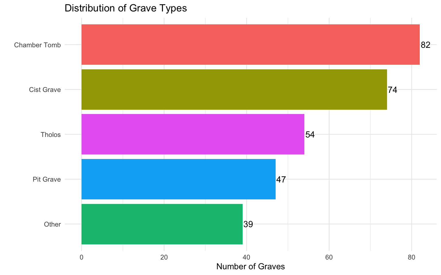
Grave Type Distribution
grave_type_summary <- cups_skulls_clean %>%
  count(grave_type_simple, name = "count") %>%
  arrange(desc(count))

print(grave_type_summary)
# A tibble: 5 × 2
grave_type_simple count
<chr> <int>
1 Chamber Tomb 82
2 Cist Grave 74
3 Tholos 54
4 Pit Grave 47
5 Other 39ggplot(grave_type_summary, aes(x = reorder(grave_type_simple, count), y = count, fill = grave_type_simple)) +
geom_col() +
coord_flip() +
geom_text(aes(label = count), hjust = -0.1, size = 4) +
labs(
title = "Distribution of Grave Types",
x = "",
y = "Number of Graves"
) +
theme_minimal() +
theme(legend.position = "none")
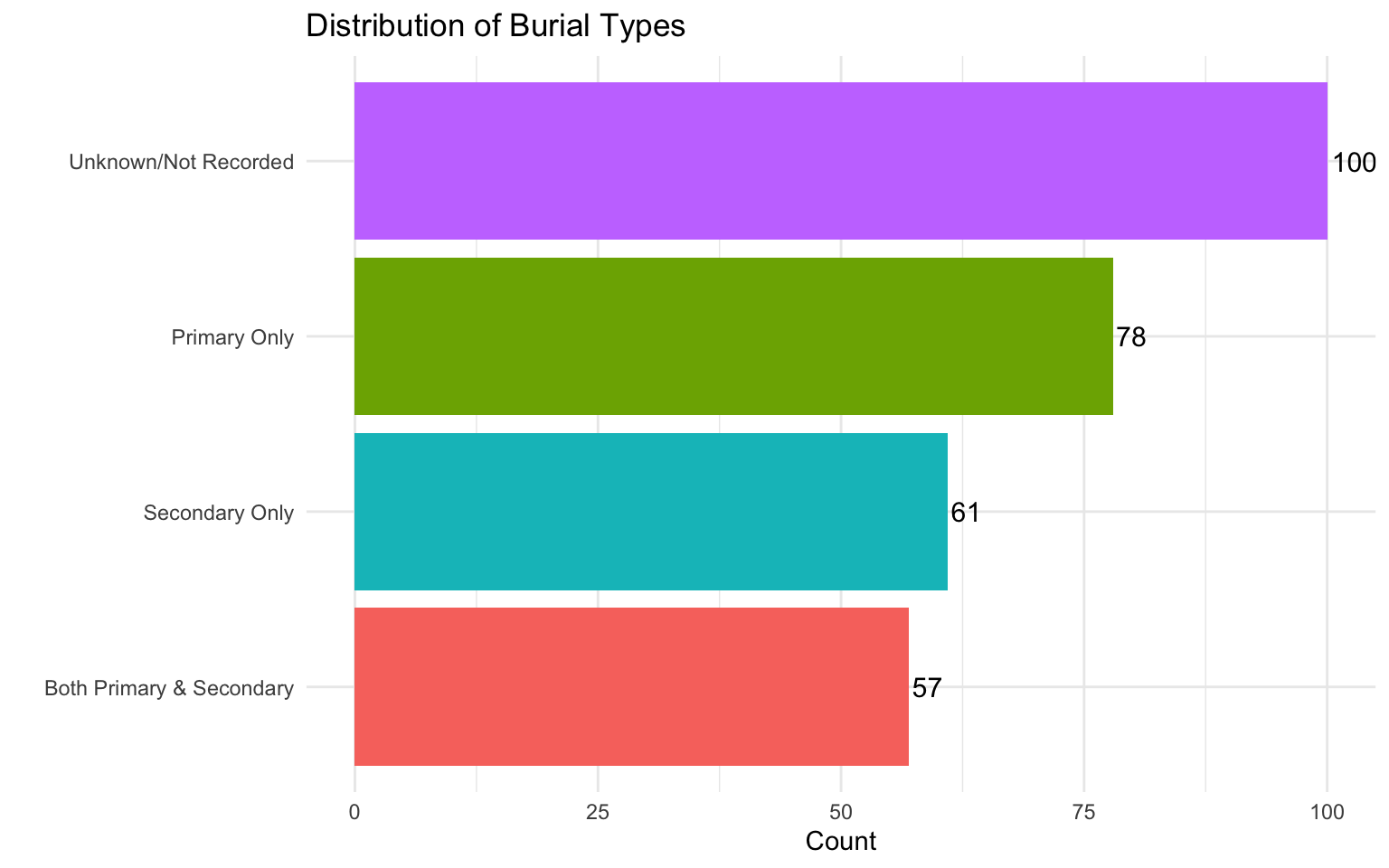
Burial Types
Primary vs Secondary Burials
burial_type_summary <- cups_skulls_clean %>%
  summarise(
    total = n(),
    with_primary = sum(primary_burial == TRUE, na.rm = TRUE),
    with_secondary = sum(secondary_burial == TRUE, na.rm = TRUE),
    both = sum(primary_burial == TRUE & secondary_burial == TRUE, na.rm = TRUE),
    neither = sum(primary_burial == FALSE & secondary_burial == FALSE, na.rm = TRUE),
    unknown = sum(is.na(primary_burial) | is.na(secondary_burial))
  ) %>%
  mutate(
    pct_primary = round(with_primary / total * 100, 1),
    pct_secondary = round(with_secondary / total * 100, 1),
    pct_both = round(both / total * 100, 1)
  )

print(burial_type_summary)
# A tibble: 1 × 9
total with_primary with_secondary both neither unknown pct_primary
<int> <int> <int> <int> <int> <int> <dbl>
1 296 135 118 57 100 0 45.6
# ℹ 2 more variables: pct_secondary <dbl>, pct_both <dbl>burial_category_data <- cups_skulls_clean %>%
count(burial_category) %>%
arrange(desc(n))
ggplot(burial_category_data, aes(x = reorder(burial_category, n), y = n, fill = burial_category)) +
geom_col() +
coord_flip() +
geom_text(aes(label = n), hjust = -0.1, size = 4) +
labs(
title = "Distribution of Burial Types",
x = "",
y = "Count"
) +
theme_minimal() +
theme(legend.position = "none")
Drinking Vessels Analysis
Overall Drinking Vessel Presence
dv_summary <- cups_skulls_clean %>%
  summarise(
    total_graves = n(),
    with_vessels = sum(has_drinking_vessel == TRUE, na.rm = TRUE),
    without_vessels = sum(has_drinking_vessel == FALSE, na.rm = TRUE),
    unknown_vessel_status = sum(is.na(has_drinking_vessel))
  ) %>%
  mutate(
    pct_with = round(with_vessels / total_graves * 100, 1),
    avg_vessels_recorded = round(mean(cups_skulls_clean$drinking_vessel_number, na.rm = TRUE), 2)
  )

print(dv_summary)
# A tibble: 1 × 6
total_graves with_vessels without_vessels unknown_vessel_status pct_with
<int> <int> <int> <int> <dbl>
1 296 80 216 0 27
# ℹ 1 more variable: avg_vessels_recorded <dbl>
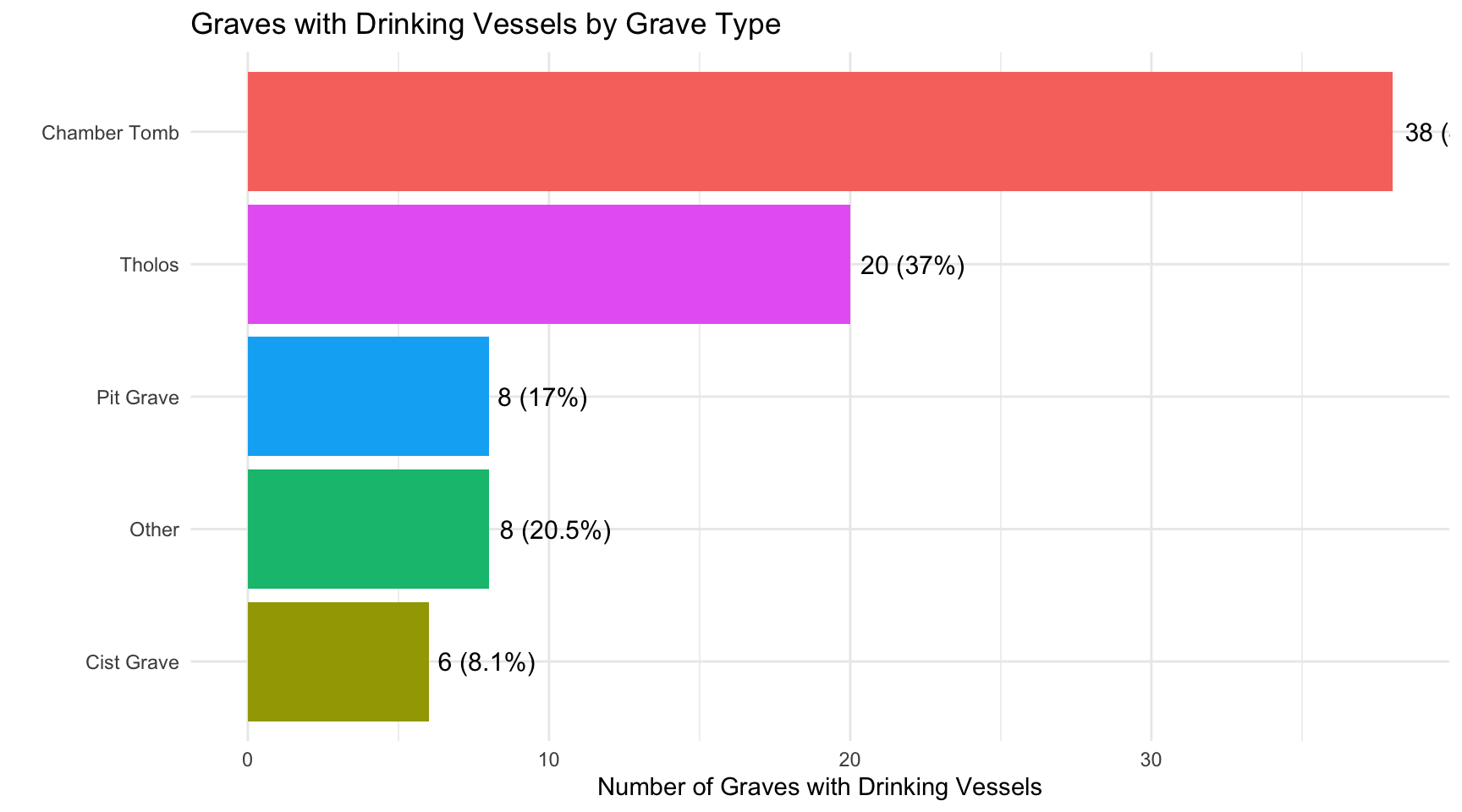
Drinking Vessels by Grave Type
dv_by_type <- cups_skulls_clean %>%
  group_by(grave_type_simple) %>%
  summarise(
    total = n(),
    with_vessels = sum(has_drinking_vessel == TRUE, na.rm = TRUE),
    pct_with_vessels = round(with_vessels / total * 100, 1),
    avg_vessel_count = round(mean(drinking_vessel_number, na.rm = TRUE), 2)
  ) %>%
  arrange(desc(with_vessels))

print(dv_by_type)
# A tibble: 5 × 5
grave_type_simple total with_vessels pct_with_vessels avg_vessel_count
<chr> <int> <int> <dbl> <dbl>
1 Chamber Tomb 82 38 46.3 2.62
2 Tholos 54 20 37 2.74
3 Other 39 8 20.5 1.25
4 Pit Grave 47 8 17 1.14
5 Cist Grave 74 6 8.1 1.33ggplot(dv_by_type, aes(x = reorder(grave_type_simple, with_vessels), y = with_vessels, fill = grave_type_simple)) +
geom_col() +
coord_flip() +
geom_text(aes(label = paste0(with_vessels, " (", pct_with_vessels, "%)")), hjust = -0.1, size = 4) +
labs(
title = "Graves with Drinking Vessels by Grave Type",
x = "",
y = "Number of Graves with Drinking Vessels"
) +
theme_minimal() +
theme(legend.position = "none")
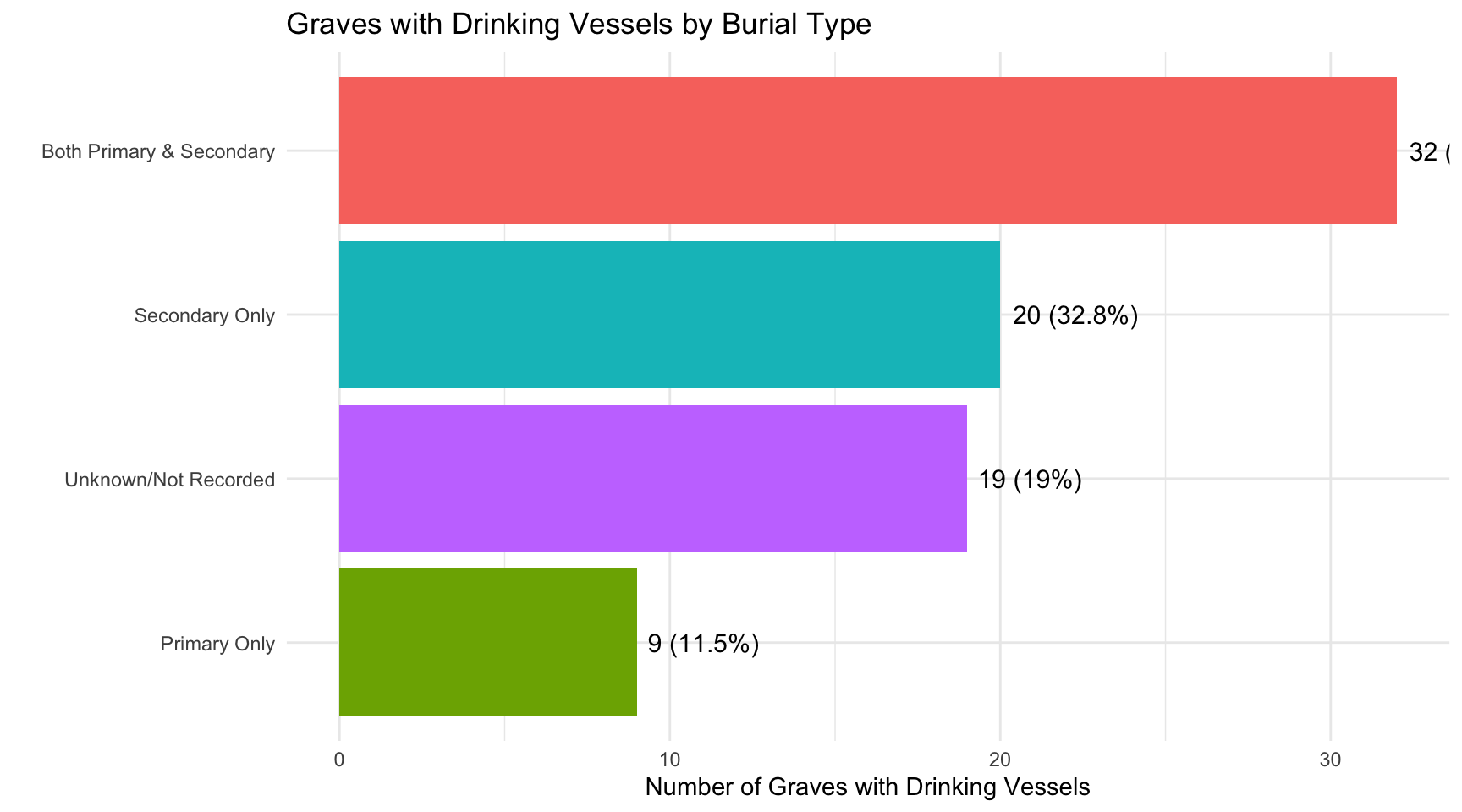
Drinking Vessels by Burial Type
dv_by_burial <- cups_skulls_clean %>%
  group_by(burial_category) %>%
  summarise(
    total = n(),
    with_vessels = sum(has_drinking_vessel == TRUE, na.rm = TRUE),
    pct_with_vessels = round(with_vessels / total * 100, 1),
    avg_vessel_count = round(mean(drinking_vessel_number, na.rm = TRUE), 2)
  ) %>%
  arrange(desc(with_vessels))

print(dv_by_burial)
# A tibble: 4 × 5
burial_category total with_vessels pct_with_vessels avg_vessel_count
<chr> <int> <int> <dbl> <dbl>
1 Both Primary & Secondary 57 32 56.1 3.1
2 Secondary Only 61 20 32.8 1.83
3 Unknown/Not Recorded 100 19 19 1.88
4 Primary Only 78 9 11.5 1 ggplot(dv_by_burial, aes(x = reorder(burial_category, with_vessels), y = with_vessels, fill = burial_category)) +
geom_col() +
coord_flip() +
geom_text(aes(label = paste0(with_vessels, " (", pct_with_vessels, "%)")), hjust = -0.1, size = 4) +
labs(
title = "Graves with Drinking Vessels by Burial Type",
x = "",
y = "Number of Graves with Drinking Vessels"
) +
theme_minimal() +
theme(legend.position = "none")
Skeletal Remains Analysis
Remains Distribution
remains_summary <- cups_skulls_clean %>%
  summarise(
    total_graves = n(),
    with_remains = sum(has_remains == TRUE, na.rm = TRUE),
    without_remains = sum(has_remains == FALSE, na.rm = TRUE),
    unknown_remains = sum(is.na(has_remains))
  ) %>%
  mutate(pct_with_remains = round(with_remains / total_graves * 100, 1))

print(remains_summary)
# A tibble: 1 × 5
total_graves with_remains without_remains unknown_remains pct_with_remains
<int> <int> <int> <int> <dbl>
1 296 226 70 0 76.4
Skulls Recorded
skulls_stats <- cups_skulls_clean %>%
  filter(!is.na(skulls_number)) %>%
  summarise(
    graves_with_skull_count = n(),
    total_skulls = sum(skulls_number, na.rm = TRUE),
    avg_skulls = round(mean(skulls_number, na.rm = TRUE), 2),
    min_skulls = min(skulls_number, na.rm = TRUE),
    max_skulls = max(skulls_number, na.rm = TRUE)
  )

print(skulls_stats)
# A tibble: 1 × 5
graves_with_skull_count total_skulls avg_skulls min_skulls max_skulls
<int> <dbl> <dbl> <dbl> <dbl>
1 83 350 4.22 1 47skulls_by_count <- cups_skulls_clean %>%
filter(!is.na(skulls_number)) %>%
count(skulls_number, name = "graves") %>%
arrange(skulls_number)
print(skulls_by_count)# A tibble: 16 × 2
skulls_number graves
<dbl> <int>
1 1 48
2 2 10
3 3 5
4 4 2
5 5 1
6 6 3
7 7 1
8 9 2
9 10 2
10 12 2
11 14 1
12 15 1
13 20 2
14 24 1
15 27 1
16 47 1
Cross-Analysis: Drinking Vessels and Remains
Do graves with drinking vessels tend to have remains?
vessels_remains_cross <- cups_skulls_clean %>%
  filter(!is.na(has_drinking_vessel) & !is.na(has_remains)) %>%
  count(has_drinking_vessel, has_remains) %>%
  pivot_wider(names_from = has_remains, values_from = n, values_fill = 0) %>%
  rename(no_remains = `FALSE`, with_remains = `TRUE`)

rownames(vessels_remains_cross) <- c("No Drinking Vessels", "With Drinking Vessels")
Warning: Setting row names on a tibble is deprecated.print(vessels_remains_cross)# A tibble: 2 × 3
has_drinking_vessel no_remains with_remains
* <lgl> <int> <int>
1 FALSE 55 161
2 TRUE 15 65# Calculate cross-tabulation with percentages
cross_analysis <- cups_skulls_clean %>%
filter(!is.na(has_drinking_vessel) & !is.na(has_remains)) %>%
group_by(has_drinking_vessel) %>%
summarise(
total = n(),
with_remains = sum(has_remains == TRUE, na.rm = TRUE),
pct_with_remains = round(with_remains / total * 100, 1)
) %>%
mutate(vessel_status = ifelse(has_drinking_vessel, "With Drinking Vessels", "Without Drinking Vessels"))
kable(select(cross_analysis, vessel_status, total, with_remains, pct_with_remains))
Without Drinking Vessels
216
161
74.5
With Drinking Vessels
80
65
81.2
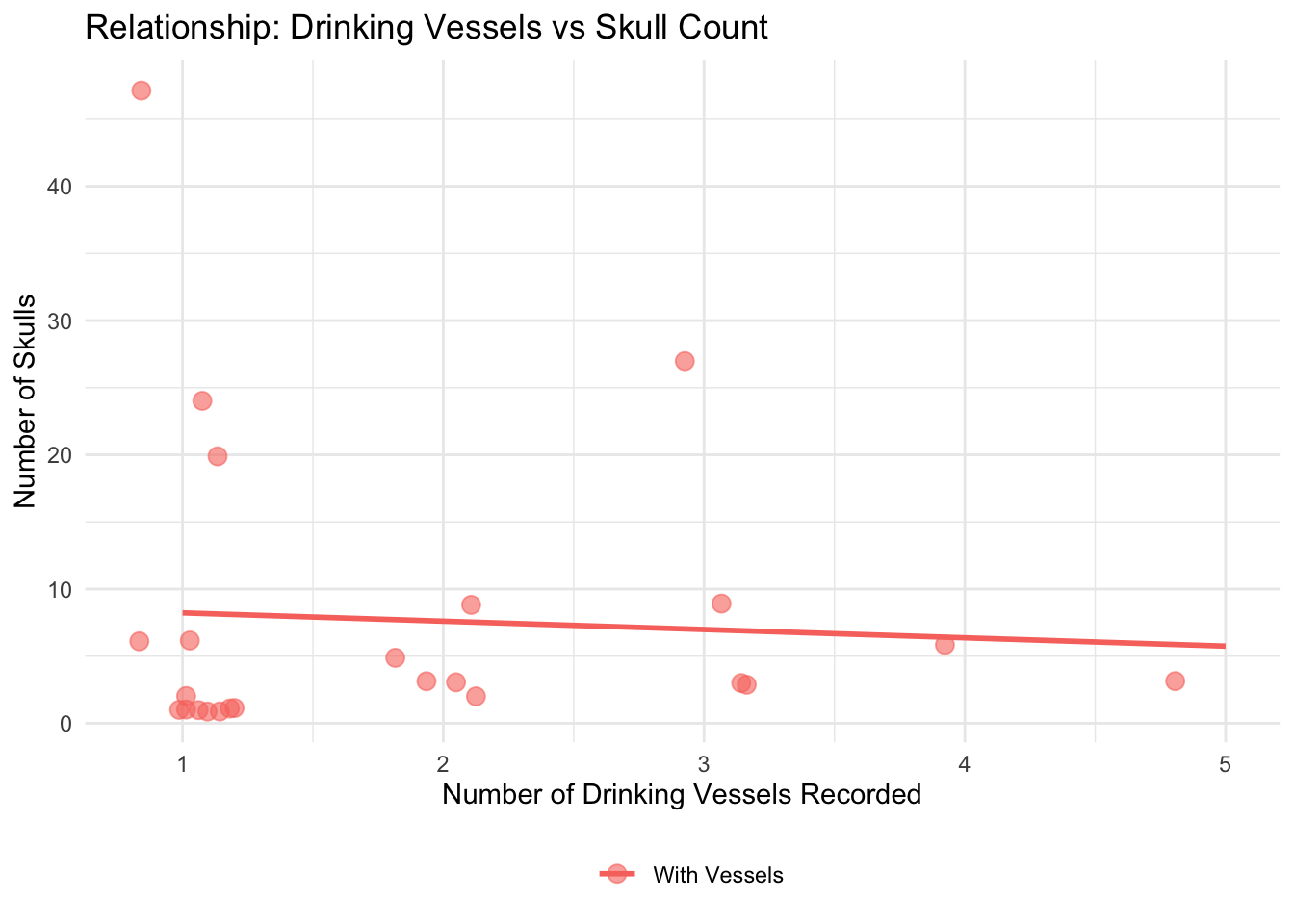
Drinking Vessels and Skull Count
vessels_skulls_data <- cups_skulls_clean %>%
  filter(!is.na(drinking_vessel_number) & !is.na(skulls_number)) %>%
  mutate(has_vessels_label = ifelse(has_drinking_vessel, "With Vessels", "No Vessels"))

ggplot(vessels_skulls_data, aes(x = drinking_vessel_number, y = skulls_number, color = has_vessels_label)) +
  geom_jitter(size = 3, alpha = 0.6, width = 0.2, height = 0.2) +
  geom_smooth(method = "lm", se = FALSE, alpha = 0.2) +
  labs(
    title = "Relationship: Drinking Vessels vs Skull Count",
    x = "Number of Drinking Vessels Recorded",
    y = "Number of Skulls",
    color = ""
  ) +
  theme_minimal() +
  theme(legend.position = "bottom")
`geom_smooth()` using formula = 'y ~ x'
Regional Analysis
Laconia vs Other Regions
regional_summary <- cups_skulls_clean %>%
  group_by(region) %>%
  summarise(
    total_graves = n(),
    with_drinking_vessels = sum(has_drinking_vessel == TRUE, na.rm = TRUE),
    pct_with_vessels = round(with_drinking_vessels / total_graves * 100, 1),
    with_remains = sum(has_remains == TRUE, na.rm = TRUE),
    pct_with_remains = round(with_remains / total_graves * 100, 1),
    avg_skulls = round(mean(skulls_number, na.rm = TRUE), 2)
  )

print(regional_summary)
# A tibble: 2 × 7
region total_graves with_drinking_vessels pct_with_vessels with_remains
<chr> <int> <int> <dbl> <int>
1 laconia 153 29 19 127
2 messenia 143 51 35.7 99
# ℹ 2 more variables: pct_with_remains <dbl>, avg_skulls <dbl>
Chronological Overview
Periods Represented
period_summary <- cups_skulls_clean %>%
  mutate(
    period_category = case_when(
      str_detect(tolower(period), "mh") ~ "Middle Helladic",
      str_detect(tolower(period), "lh\\s*i(?!i)")  | str_detect(tolower(period), "lh i-") ~ "LH I-II",
      str_detect(tolower(period), "lh\\s*ii") & !str_detect(tolower(period), "lh\\s*ii") ~ "LH II",
      str_detect(tolower(period), "lh\\s*iii") ~ "LH III",
      str_detect(tolower(period), "lh") ~ "Late Helladic (general)",
      is.na(period) | period == "" ~ "Unrecorded",
      TRUE ~ "Other"
    )
  ) %>%
  count(period_category, name = "graves") %>%
  arrange(desc(graves))

print(period_summary)
# A tibble: 5 × 2
period_category graves
<chr> <int>
1 Unrecorded 90
2 LH III 88
3 LH I-II 45
4 Middle Helladic 39
5 Late Helladic (general) 34
Key Findings Summary
cat("=== KEY FINDINGS ===\n\n")=== KEY FINDINGS ===cat("1. Drinking Vessel Prevalence:\n")1. Drinking Vessel Prevalence:cat(" -", sum(cups_skulls_clean$has_drinking_vessel == TRUE, na.rm = TRUE),
"graves (", round(sum(cups_skulls_clean$has_drinking_vessel == TRUE, na.rm = TRUE) / nrow(cups_skulls_clean) * 100, 1),
"%) have drinking vessels recorded\n\n") - 80 graves ( 27 %) have drinking vessels recordedcat("2. Skeletal Remains:\n")2. Skeletal Remains:cat(" -", sum(cups_skulls_clean$has_remains == TRUE, na.rm = TRUE),
"graves (", round(sum(cups_skulls_clean$has_remains == TRUE, na.rm = TRUE) / nrow(cups_skulls_clean) * 100, 1),
"%) have human remains\n") - 226 graves ( 76.4 %) have human remainscat(" - Skull counts recorded in", sum(!is.na(cups_skulls_clean$skulls_number)), "graves\n\n") - Skull counts recorded in 83 gravescat("3. Burial Type Association:\n")3. Burial Type Association:burial_counts <- cups_skulls_clean %>%
count(burial_category) %>%
arrange(desc(n))
for (i in 1:nrow(burial_counts)) {
cat(" -", burial_counts$burial_category[i], ":", burial_counts$n[i], "graves\n")
} - Unknown/Not Recorded : 100 graves
- Primary Only : 78 graves
- Secondary Only : 61 graves
- Both Primary & Secondary : 57 graves
Chamber Space and Burial Goods
Do larger chambers have more skulls and drinking vessels?
This section explores whether the estimated chamber area relates to
the number of skulls and drinking vessels found.
Data Availability
space_analysis_data <- cups_skulls_clean %>%
  filter(!is.na(area_of_chamber_estimated))

cat("Graves with chamber area estimated:", nrow(space_analysis_data), "\n")
Graves with chamber area estimated: 99 cat("Graves with area AND skull count:", sum(!is.na(space_analysis_data$skulls_number)), "\n")Graves with area AND skull count: 22 cat("Graves with area AND vessel count:", sum(!is.na(space_analysis_data$drinking_vessel_number)), "\n\n")Graves with area AND vessel count: 41 # Summary statistics for chamber area
cat("Chamber Area Summary (m²):\n")Chamber Area Summary (m²):print(space_analysis_data %>%
pull(area_of_chamber_estimated) %>%
summary()) Min. 1st Qu. Median Mean 3rd Qu. Max.
1.419 7.069 12.566 19.056 23.330 88.250
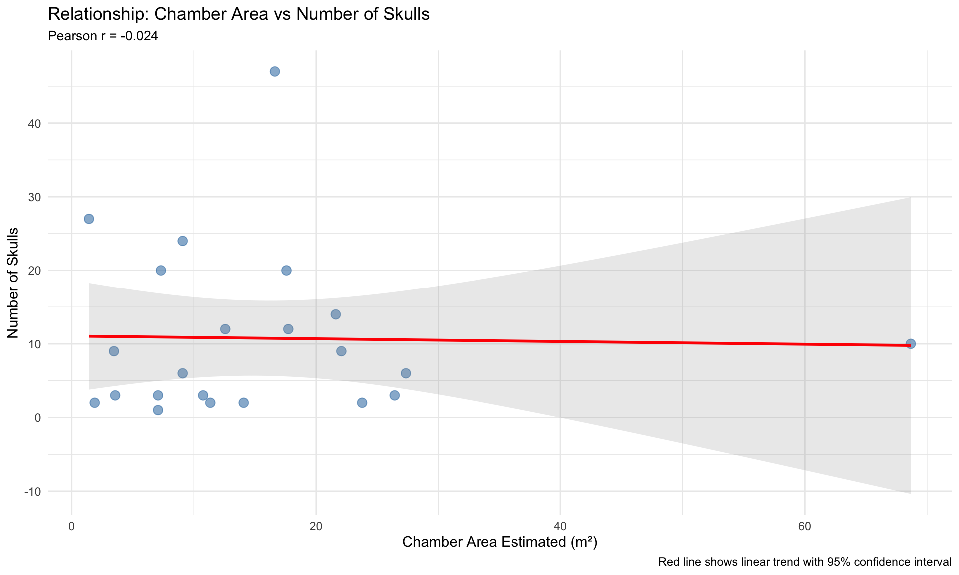
Skulls vs Chamber Area
skulls_area_data <- cups_skulls_clean %>%
  filter(!is.na(area_of_chamber_estimated) & !is.na(skulls_number))

# Calculate correlation
cor_skulls_area <- cor(skulls_area_data$area_of_chamber_estimated, skulls_area_data$skulls_number, use = "complete.obs")

ggplot(skulls_area_data, aes(x = area_of_chamber_estimated, y = skulls_number)) +
  geom_point(size = 3, alpha = 0.6, color = "steelblue") +
  geom_smooth(method = "lm", se = TRUE, color = "red", alpha = 0.2) +
  labs(
    title = "Relationship: Chamber Area vs Number of Skulls",
    subtitle = paste0("Pearson r = ", round(cor_skulls_area, 3)),
    x = "Chamber Area Estimated (m²)",
    y = "Number of Skulls",
    caption = "Red line shows linear trend with 95% confidence interval"
  ) +
  theme_minimal() +
  theme(plot.subtitle = element_text(size = 10))
`geom_smooth()` using formula = 'y ~ x'
# Statistical test
skulls_lm <- lm(skulls_number ~ area_of_chamber_estimated, data = skulls_area_data)
skulls_summary <- summary(skulls_lm)

cat("Linear Model: Skulls ~ Chamber Area\n")
Linear Model: Skulls ~ Chamber Areaprint(skulls_summary)
Call:
lm(formula = skulls_number ~ area_of_chamber_estimated, data = skulls_area_data)

Residuals:
   Min     1Q Median     3Q    Max
-9.929 -7.978 -3.274  2.823 36.249

Coefficients:
                          Estimate Std. Error t value Pr(>|t|)
(Intercept)               11.06009    3.65712   3.024   0.0067 **
area_of_chamber_estimated -0.01857    0.17576  -0.106   0.9169
---
Signif. codes:  0 '***' 0.001 '**' 0.01 '*' 0.05 '.' 0.1 ' ' 1

Residual standard error: 11.47 on 20 degrees of freedom
Multiple R-squared:  0.0005579, Adjusted R-squared:  -0.04941
F-statistic: 0.01116 on 1 and 20 DF,  p-value: 0.9169
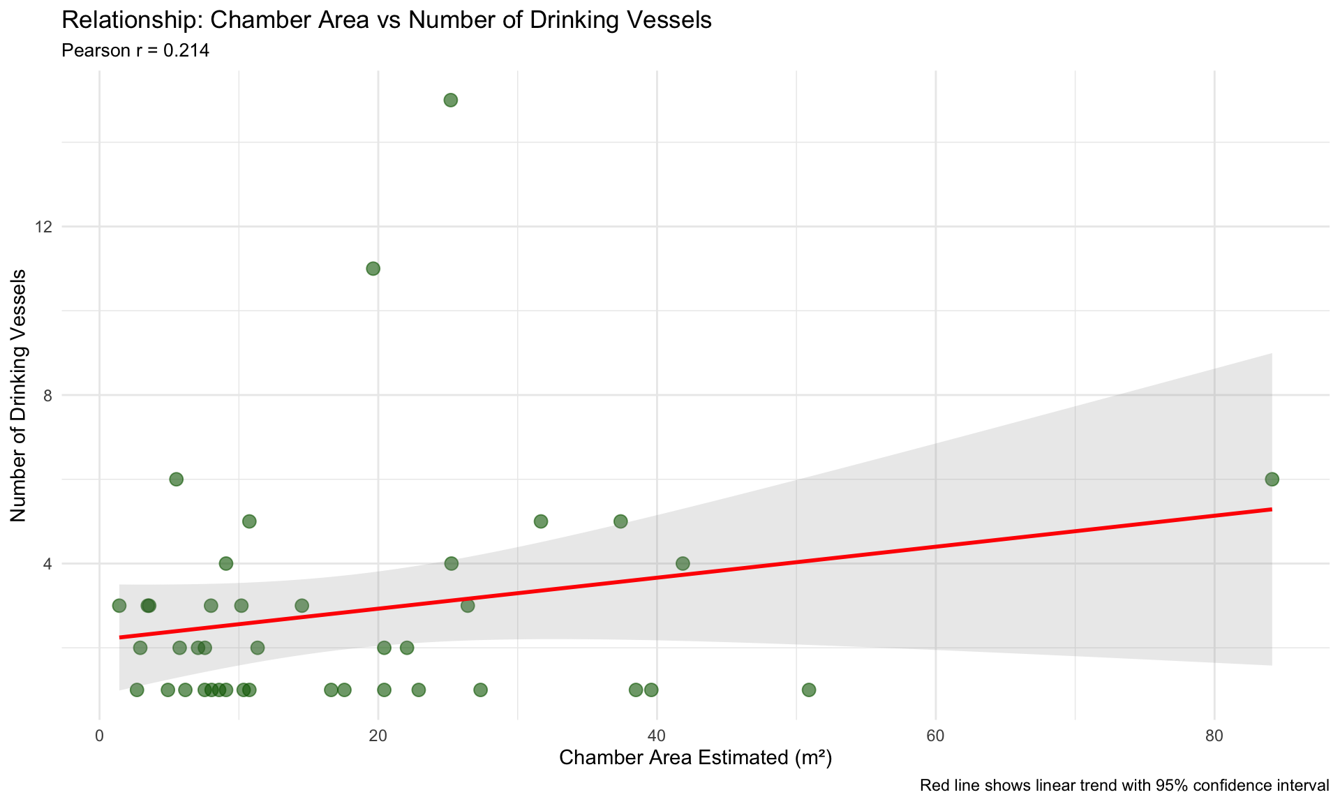
Drinking Vessels vs Chamber Area
vessels_area_data <- cups_skulls_clean %>%
  filter(!is.na(area_of_chamber_estimated) & !is.na(drinking_vessel_number))

# Calculate correlation
cor_vessels_area <- cor(vessels_area_data$area_of_chamber_estimated, vessels_area_data$drinking_vessel_number, use = "complete.obs")

ggplot(vessels_area_data, aes(x = area_of_chamber_estimated, y = drinking_vessel_number)) +
  geom_point(size = 3, alpha = 0.6, color = "darkgreen") +
  geom_smooth(method = "lm", se = TRUE, color = "red", alpha = 0.2) +
  labs(
    title = "Relationship: Chamber Area vs Number of Drinking Vessels",
    subtitle = paste0("Pearson r = ", round(cor_vessels_area, 3)),
    x = "Chamber Area Estimated (m²)",
    y = "Number of Drinking Vessels",
    caption = "Red line shows linear trend with 95% confidence interval"
  ) +
  theme_minimal() +
  theme(plot.subtitle = element_text(size = 10))
`geom_smooth()` using formula = 'y ~ x'
# Statistical test
vessels_lm <- lm(drinking_vessel_number ~ area_of_chamber_estimated, data = vessels_area_data)
vessels_summary <- summary(vessels_lm)

cat("Linear Model: Drinking Vessels ~ Chamber Area\n")
Linear Model: Drinking Vessels ~ Chamber Areaprint(vessels_summary)
Call:
lm(formula = drinking_vessel_number ~ area_of_chamber_estimated,
    data = vessels_area_data)

Residuals:
    Min      1Q  Median      3Q     Max
-3.0646 -1.5264 -0.4705  0.6802 11.8807

Coefficients:
                          Estimate Std. Error t value Pr(>|t|)
(Intercept)                2.19238    0.64999   3.373  0.00169 **
area_of_chamber_estimated  0.03678    0.02693   1.366  0.17982
---
Signif. codes:  0 '***' 0.001 '**' 0.01 '*' 0.05 '.' 0.1 ' ' 1

Residual standard error: 2.777 on 39 degrees of freedom
Multiple R-squared:  0.04565,   Adjusted R-squared:  0.02118
F-statistic: 1.865 on 1 and 39 DF,  p-value: 0.1798
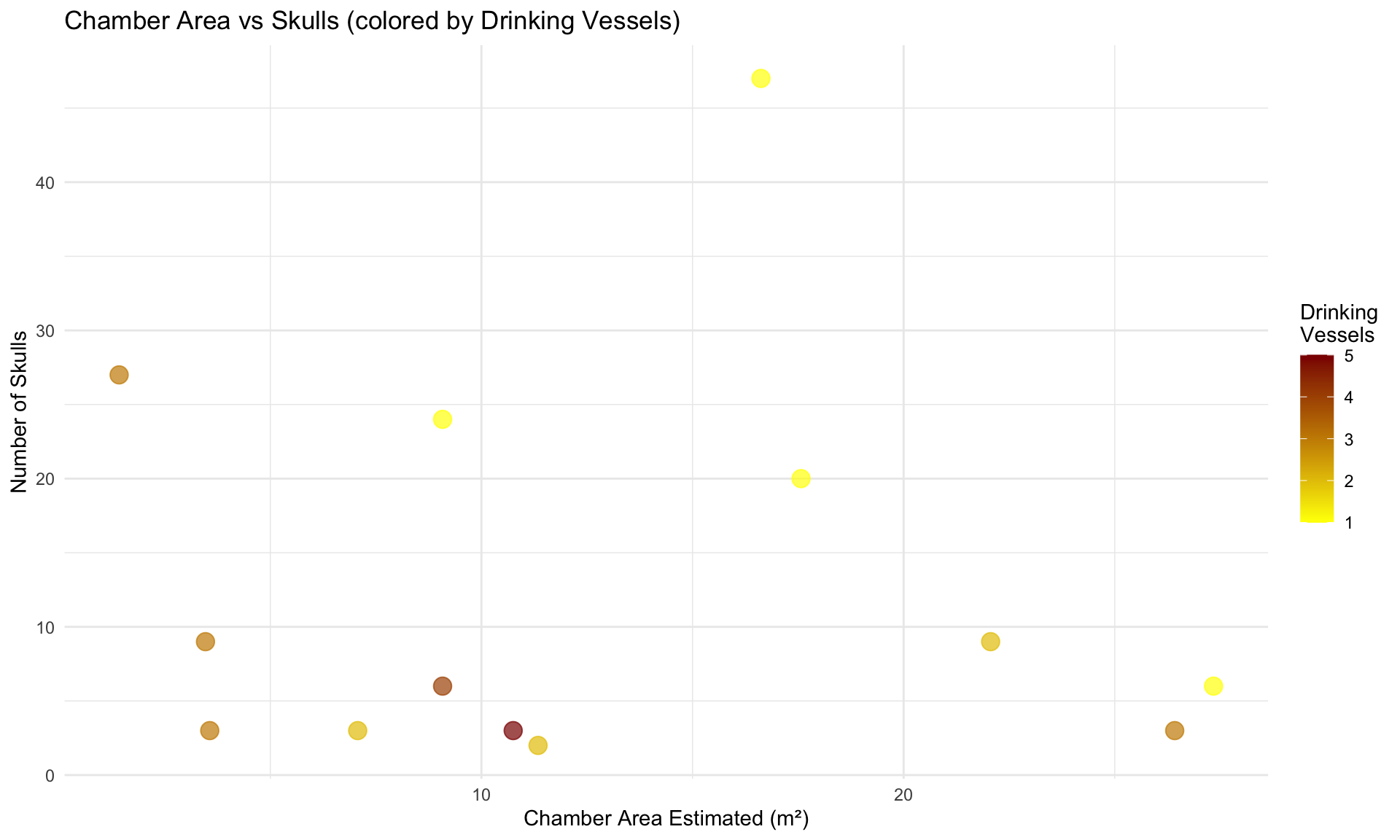
Both Skulls and Vessels vs Chamber Area
both_area_data <- cups_skulls_clean %>%
  filter(!is.na(area_of_chamber_estimated) & !is.na(skulls_number) & !is.na(drinking_vessel_number))

ggplot(both_area_data, aes(x = area_of_chamber_estimated, y = skulls_number)) +
  geom_point(aes(color = drinking_vessel_number), size = 4, alpha = 0.7) +
  scale_color_gradient(name = "Drinking\nVessels", low = "yellow", high = "darkred") +
  labs(
    title = "Chamber Area vs Skulls (colored by Drinking Vessels)",
    x = "Chamber Area Estimated (m²)",
    y = "Number of Skulls"
  ) +
  theme_minimal()
Session Info
sessionInfo()R version 4.5.2 (2025-10-31)
Platform: aarch64-apple-darwin20
Running under: macOS Tahoe 26.2
Matrix products: default
BLAS: /System/Library/Frameworks/Accelerate.framework/Versions/A/Frameworks/vecLib.framework/Versions/A/libBLAS.dylib
LAPACK: /Library/Frameworks/R.framework/Versions/4.5-arm64/Resources/lib/libRlapack.dylib; LAPACK version 3.12.1
locale:
[1] en_US/en_US/en_US/C/en_US/en_US
time zone: America/Detroit
tzcode source: internal
attached base packages:
[1] stats graphics grDevices datasets utils methods base
other attached packages:
[1] knitr_1.50 janitor_2.2.1 tidyr_1.3.1 ggplot2_4.0.1 dplyr_1.1.4
[6] readr_2.1.5 stringr_1.6.0
loaded via a namespace (and not attached):
[1] utf8_1.2.6 sass_0.4.10 generics_0.1.4 renv_1.1.6
[5] lattice_0.22-7 stringi_1.8.7 hms_1.1.3 digest_0.6.37
[9] magrittr_2.0.4 evaluate_1.0.3 grid_4.5.2 timechange_0.3.0
[13] RColorBrewer_1.1-3 fastmap_1.2.0 Matrix_1.7-4 rprojroot_2.0.4
[17] workflowr_1.7.1 jsonlite_2.0.0 whisker_0.4.1 promises_1.3.3
[21] mgcv_1.9-3 purrr_1.2.0 scales_1.4.0 jquerylib_0.1.4
[25] cli_3.6.5 crayon_1.5.3 rlang_1.1.7 splines_4.5.2
[29] bit64_4.6.0-1 withr_3.0.2 cachem_1.1.0 yaml_2.3.10
[33] parallel_4.5.2 tools_4.5.2 tzdb_0.5.0 httpuv_1.6.16
[37] here_1.0.1 vctrs_0.7.1 R6_2.6.1 lifecycle_1.0.5
[41] lubridate_1.9.4 git2r_0.36.2 snakecase_0.11.1 bit_4.6.0
[45] fs_1.6.6 vroom_1.6.5 pkgconfig_2.0.3 pillar_1.11.1
[49] bslib_0.9.0 later_1.4.2 gtable_0.3.6 glue_1.8.0
[53] Rcpp_1.1.1 xfun_0.54 tibble_3.3.1 tidyselect_1.2.1
[57] dichromat_2.0-0.1 farver_2.1.2 nlme_3.1-168 htmltools_0.5.8.1
[61] labeling_0.4.3 rmarkdown_2.29 compiler_4.5.2 S7_0.2.0