Short Range Familial Search
Tina Lasisi
2023-05-21 20:49:32
Last updated: 2023-05-21
Checks: 6 1
Knit directory: PODFRIDGE/
This reproducible R Markdown analysis was created with workflowr (version 1.7.0). The Checks tab describes the reproducibility checks that were applied when the results were created. The Past versions tab lists the development history.
The R Markdown is untracked by Git. To know which version of the R
Markdown file created these results, you’ll want to first commit it to
the Git repo. If you’re still working on the analysis, you can ignore
this warning. When you’re finished, you can run
wflow_publish to commit the R Markdown file and build the
HTML.
Great job! The global environment was empty. Objects defined in the global environment can affect the analysis in your R Markdown file in unknown ways. For reproduciblity it’s best to always run the code in an empty environment.
The command set.seed(20230302) was run prior to running
the code in the R Markdown file. Setting a seed ensures that any results
that rely on randomness, e.g. subsampling or permutations, are
reproducible.
Great job! Recording the operating system, R version, and package versions is critical for reproducibility.
Nice! There were no cached chunks for this analysis, so you can be confident that you successfully produced the results during this run.
Great job! Using relative paths to the files within your workflowr project makes it easier to run your code on other machines.
Great! You are using Git for version control. Tracking code development and connecting the code version to the results is critical for reproducibility.
The results in this page were generated with repository version 10423d8. See the Past versions tab to see a history of the changes made to the R Markdown and HTML files.
Note that you need to be careful to ensure that all relevant files for
the analysis have been committed to Git prior to generating the results
(you can use wflow_publish or
wflow_git_commit). workflowr only checks the R Markdown
file, but you know if there are other scripts or data files that it
depends on. Below is the status of the Git repository when the results
were generated:
Ignored files:
    Ignored:    .DS_Store
    Ignored:    .Rhistory
    Ignored:    .Rproj.user/
    Ignored:    data/.DS_Store
    Ignored:    data/FGG_Database_v.2022.xlsx

Untracked files:
    Untracked:  1036 revised AfAm, n=342.csv
    Untracked:  1036 revised Asian, n=97.csv
    Untracked:  1036 revised Cauc, n=361.csv
    Untracked:  1036 revised Hispanic, n=236.csv
    Untracked:  1036 revised all, n=1036.csv
    Untracked:  analysis/shortrange.Rmd
    Untracked:  data/1036_AfAm.csv
    Untracked:  data/1036_Asian.csv
    Untracked:  data/1036_Cauc.csv
    Untracked:  data/1036_Hispanic.csv
    Untracked:  data/1036_all.csv
    Untracked:  data/1036_allelefreqs.xlsx
    Untracked:  data/1036_rawgeno.xlsx
    Untracked:  data/FGGUserManual2022.pdf
    Untracked:  data/~$1036_allelefreqs.xlsx
Note that any generated files, e.g. HTML, png, CSS, etc., are not included in this status report because it is ok for generated content to have uncommitted changes.
There are no past versions. Publish this analysis with
wflow_publish() to start tracking its development.
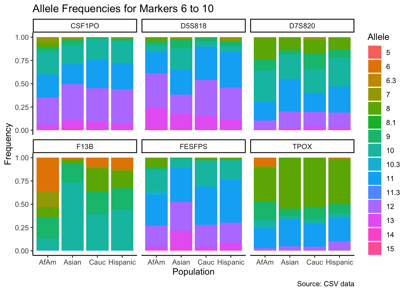
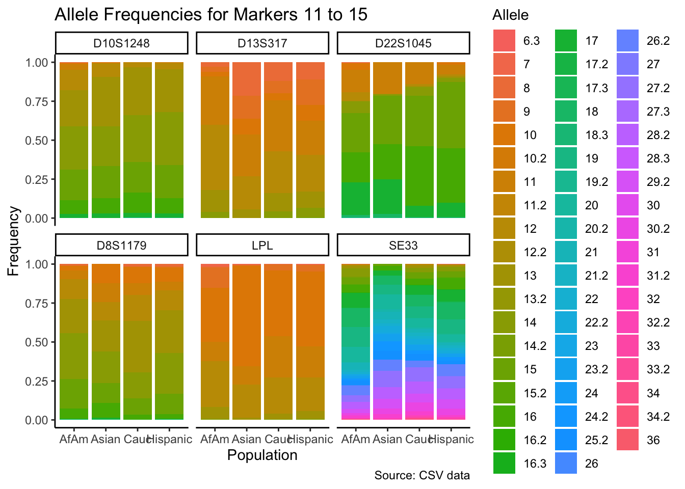
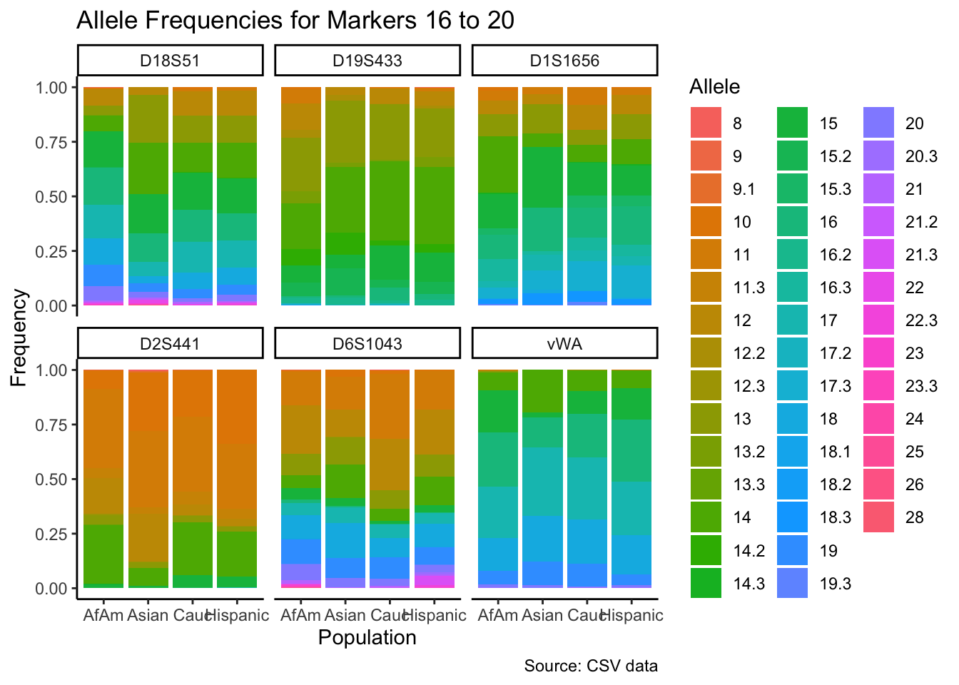
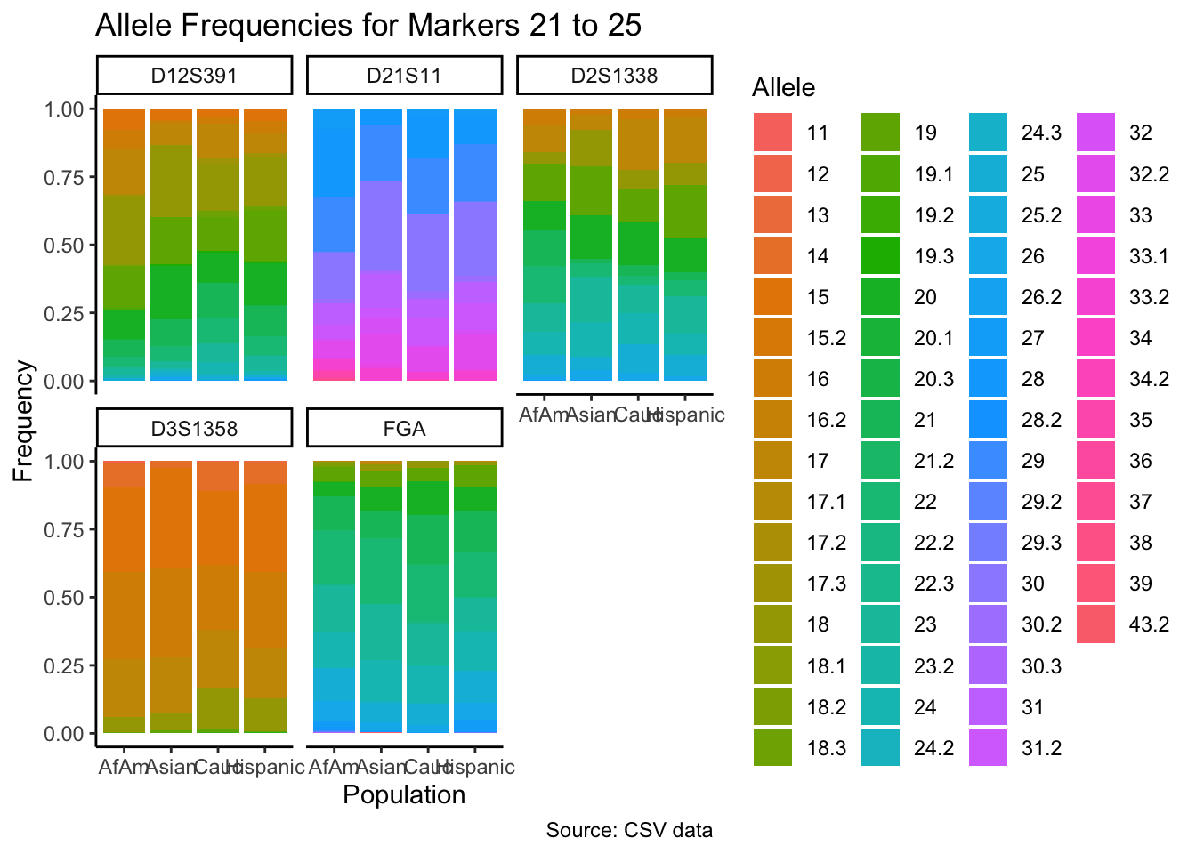
CODIS marker allele frequencies
Frequencies and raw genotypes for different populations were found here and refer to Steffen, C.R., Coble, M.D., Gettings, K.B., Vallone, P.M. (2017) Corrigendum to ‘U.S. Population Data for 29 Autosomal STR Loci’ [Forensic Sci. Int. Genet. 7 (2013) e82-e83]. Forensic Sci. Int. Genet. 31, e36–e40. The US core CODIS markers are a subset of the 29 described here.
Load CODIS allele frequencies
# Define the file paths
file_paths <- list.files(path = "data", pattern = "1036_.*\\.csv", full.names = TRUE)

# Create a list of data frames
df_list <- lapply(file_paths, function(path) {
  read_csv(path, col_types = cols(
    marker = col_character(),
    allele = col_double(),
    frequency = col_double(),
    population = col_character()
  ))
})

# Bind all data frames into one
df <- bind_rows(df_list)
# Find unique markers and split them into chunks of 5
unique_markers <- unique(df$marker)
marker_chunks <- split(unique_markers, ceiling(seq_along(unique_markers)/5))
# Loop through the chunks and create a plot for each chunk
for(i in seq_along(marker_chunks)) {
df_chunk <- df %>% filter(marker %in% marker_chunks[[i]])
p <- ggplot(df_chunk, aes(x = allele, y = frequency, fill = population)) +
geom_col(position = "dodge", width = 0.7) +
facet_grid(population ~ marker) +
# scale_x_continuous(breaks = seq(2.2, 43.2, by = 1)) +
labs(x = "Allele", y = "Frequency",
title = paste("Allele Frequencies for Markers", i*5-4, "to", min(i*5, length(unique_markers))),
caption = "Source: CSV data") +
theme_bw()
print(p)
}Warning: `position_dodge()` requires non-overlapping x intervals
`position_dodge()` requires non-overlapping x intervals
`position_dodge()` requires non-overlapping x intervals
`position_dodge()` requires non-overlapping x intervals
`position_dodge()` requires non-overlapping x intervals
`position_dodge()` requires non-overlapping x intervals
`position_dodge()` requires non-overlapping x intervals
`position_dodge()` requires non-overlapping x intervals
`position_dodge()` requires non-overlapping x intervals
`position_dodge()` requires non-overlapping x intervals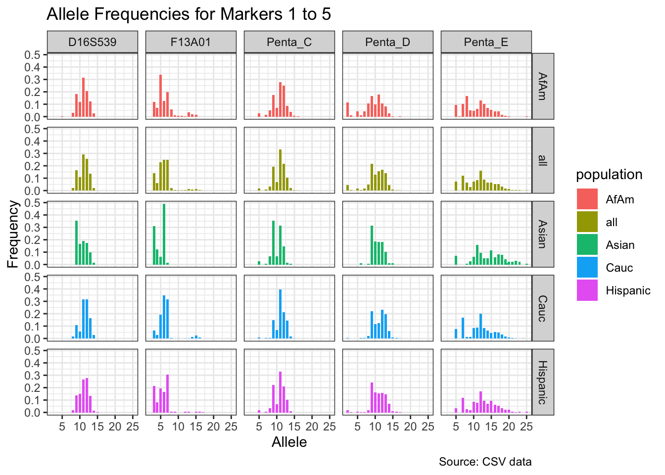
Warning: `position_dodge()` requires non-overlapping x intervals
`position_dodge()` requires non-overlapping x intervals
`position_dodge()` requires non-overlapping x intervals
`position_dodge()` requires non-overlapping x intervals
`position_dodge()` requires non-overlapping x intervals
`position_dodge()` requires non-overlapping x intervals
`position_dodge()` requires non-overlapping x intervals
`position_dodge()` requires non-overlapping x intervals
`position_dodge()` requires non-overlapping x intervals
`position_dodge()` requires non-overlapping x intervals
`position_dodge()` requires non-overlapping x intervals
`position_dodge()` requires non-overlapping x intervals
`position_dodge()` requires non-overlapping x intervals
`position_dodge()` requires non-overlapping x intervals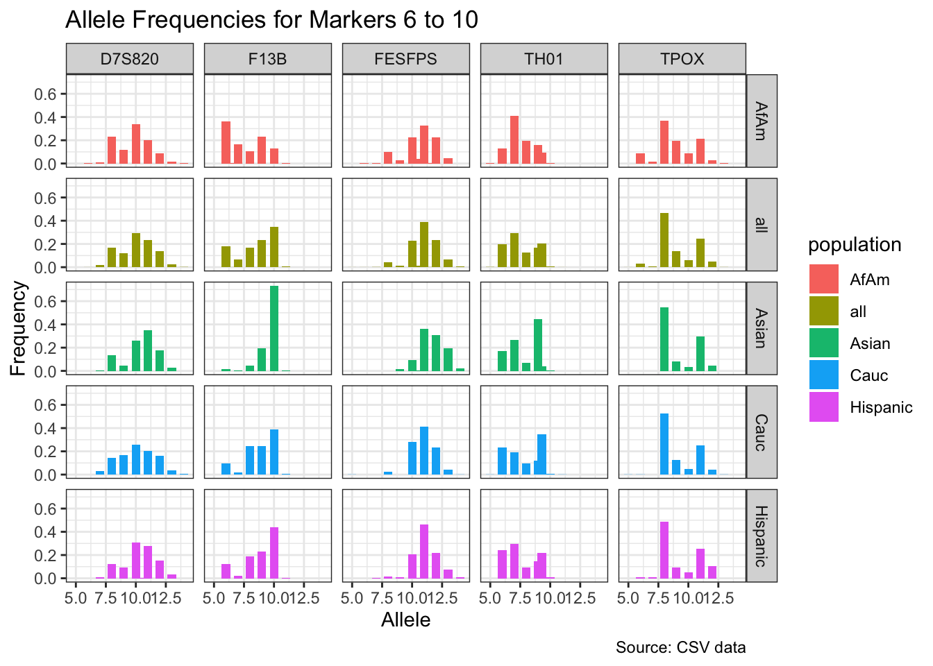
Warning: `position_dodge()` requires non-overlapping x intervals
`position_dodge()` requires non-overlapping x intervals
`position_dodge()` requires non-overlapping x intervals
`position_dodge()` requires non-overlapping x intervals
`position_dodge()` requires non-overlapping x intervals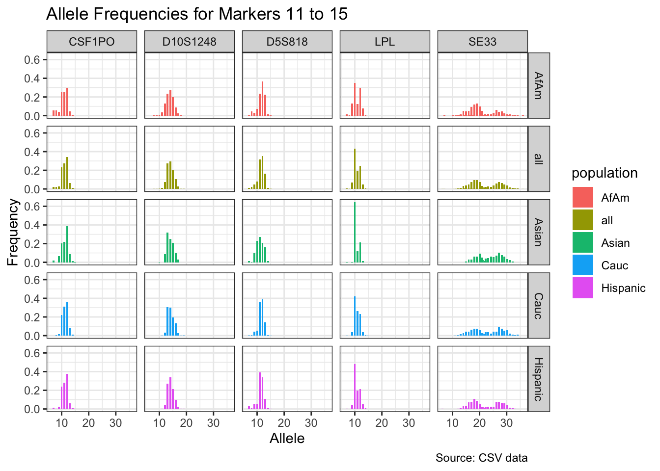
Warning: `position_dodge()` requires non-overlapping x intervals
`position_dodge()` requires non-overlapping x intervals
`position_dodge()` requires non-overlapping x intervals
`position_dodge()` requires non-overlapping x intervals
`position_dodge()` requires non-overlapping x intervals
`position_dodge()` requires non-overlapping x intervals
`position_dodge()` requires non-overlapping x intervals
`position_dodge()` requires non-overlapping x intervals
`position_dodge()` requires non-overlapping x intervals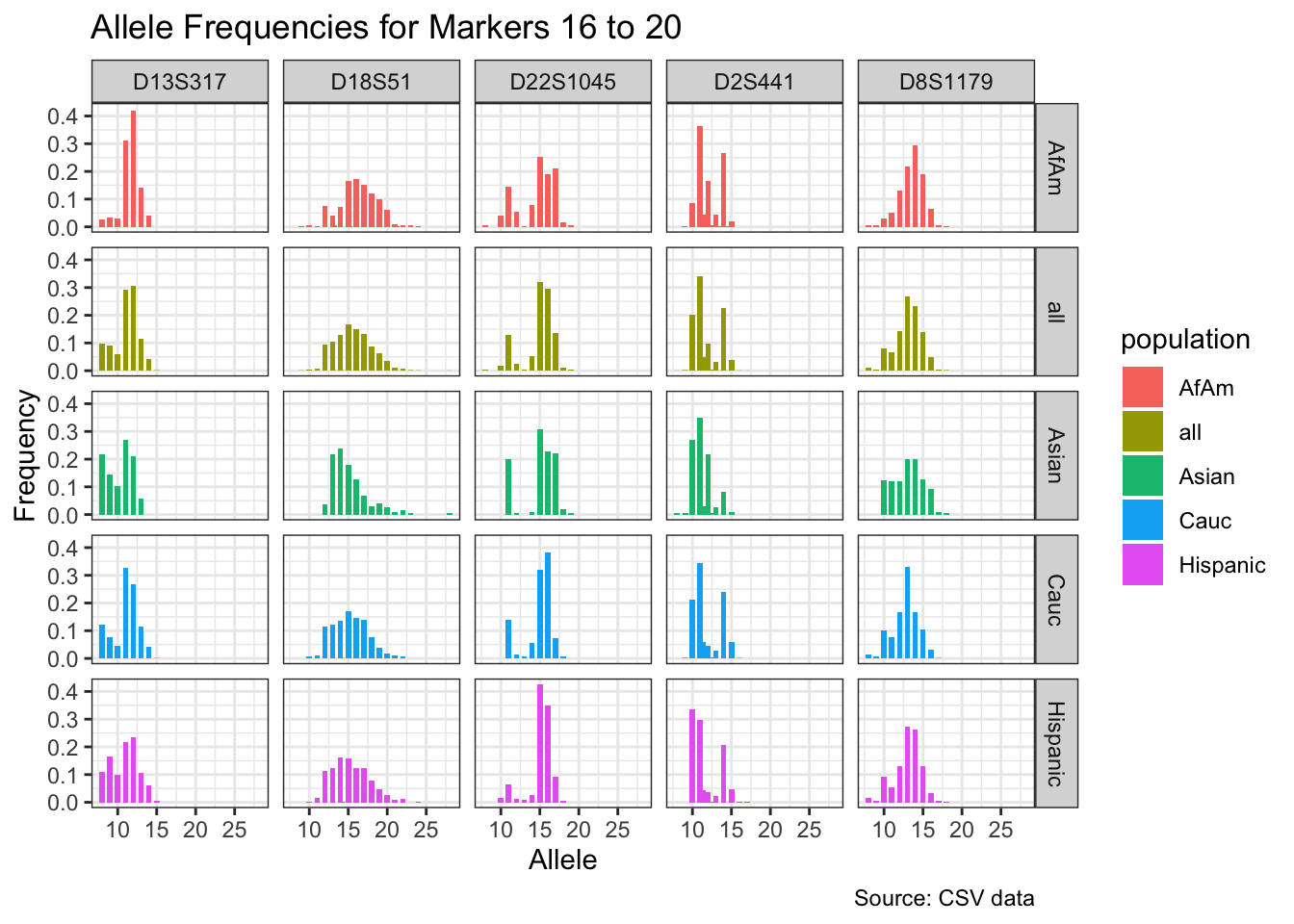
`position_dodge()` requires non-overlapping x intervals
`position_dodge()` requires non-overlapping x intervals
`position_dodge()` requires non-overlapping x intervals
`position_dodge()` requires non-overlapping x intervals
`position_dodge()` requires non-overlapping x intervals
`position_dodge()` requires non-overlapping x intervals
`position_dodge()` requires non-overlapping x intervals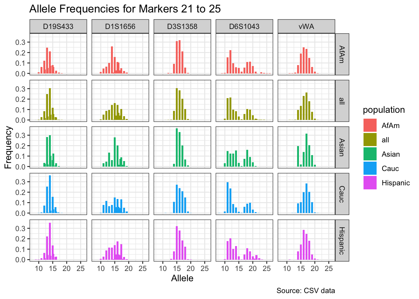
Warning: `position_dodge()` requires non-overlapping x intervals
`position_dodge()` requires non-overlapping x intervals
`position_dodge()` requires non-overlapping x intervals
`position_dodge()` requires non-overlapping x intervals
`position_dodge()` requires non-overlapping x intervals
`position_dodge()` requires non-overlapping x intervals
`position_dodge()` requires non-overlapping x intervals
`position_dodge()` requires non-overlapping x intervals
`position_dodge()` requires non-overlapping x intervals
`position_dodge()` requires non-overlapping x intervals
`position_dodge()` requires non-overlapping x intervals
`position_dodge()` requires non-overlapping x intervals
`position_dodge()` requires non-overlapping x intervals
`position_dodge()` requires non-overlapping x intervals
`position_dodge()` requires non-overlapping x intervals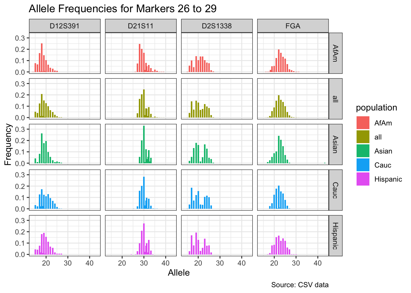
df %>%
  group_by(population) %>%
  filter(population != "all") %>%
  ggplot(aes(x = marker, y = allele, fill = population)) +
  geom_boxplot() +
  labs(x = "Marker", y = "Allele",
       title = "Range of Alleles Across Different Markers (Grouped by Population)",
       caption = "Source: CSV data") +
  coord_flip()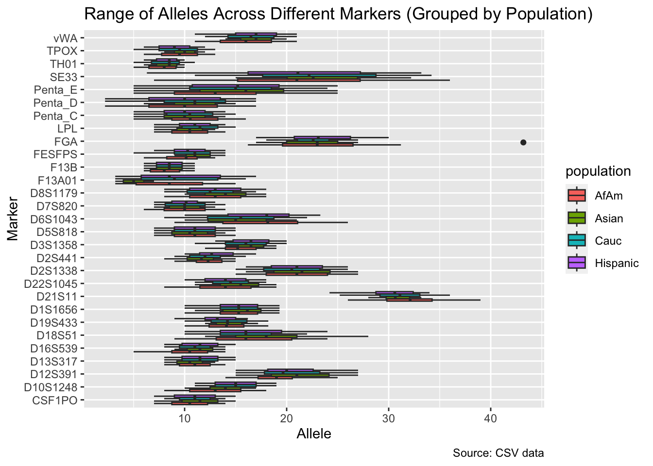
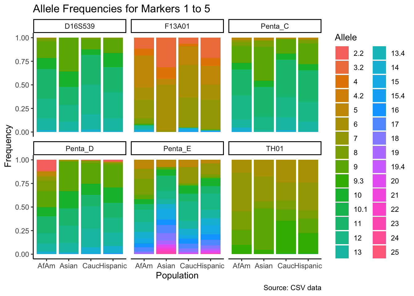
# Filter out the "all" population
df_filtered <- df %>% filter(population != "all")

# Get the unique markers and split them into chunks of 5
unique_markers <- unique(df_filtered$marker)
marker_chunks <- split(unique_markers, ceiling(seq_along(unique_markers)/6))

# Loop through the chunks
for(i in seq_along(marker_chunks)) {

  # Subset the data for the current chunk of markers
  df_chunk <- df_filtered %>% filter(marker %in% marker_chunks[[i]])

  # Convert the allele variable to a factor
  df_chunk$allele <- as.factor(df_chunk$allele)

  # Create the plot
  p <- ggplot(df_chunk, aes(x = population, y = frequency, fill = allele)) +
    geom_bar(stat = "identity") +
    facet_wrap(~ marker) +
    labs(x = "Population", y = "Frequency", fill = "Allele",
         title = paste("Allele Frequencies for Markers", i*5-4, "to", min(i*5, length(unique_markers))),
         caption = "Source: CSV data") +
    theme_classic()  # Apply theme_classic()

  # Print the plot
  print(p)
}
summary_df <- df %>%
  group_by(marker, population) %>%
  summarise(num_alleles = n_distinct(allele))
`summarise()` has grouped output by 'marker'. You can override using the
`.groups` argument.summary_df# A tibble: 145 × 3
# Groups: marker [29]
marker population num_alleles
<chr> <chr> <int>
1 CSF1PO AfAm 8
2 CSF1PO Asian 8
3 CSF1PO Cauc 7
4 CSF1PO Hispanic 9
5 CSF1PO all 9
6 D10S1248 AfAm 11
7 D10S1248 Asian 7
8 D10S1248 Cauc 9
9 D10S1248 Hispanic 9
10 D10S1248 all 12
# ℹ 135 more rowssummary_df <- df %>%
group_by(marker, population) %>%
summarise(num_alleles = n_distinct(allele))`summarise()` has grouped output by 'marker'. You can override using the
`.groups` argument.summary_pivot <- summary_df %>%
pivot_wider(names_from = population, values_from = num_alleles)
summary_pivot# A tibble: 29 × 6
# Groups: marker [29]
marker AfAm Asian Cauc Hispanic all
<chr> <int> <int> <int> <int> <int>
1 CSF1PO 8 8 7 9 9
2 D10S1248 11 7 9 9 12
3 D12S391 19 15 16 19 24
4 D13S317 7 6 8 8 8
5 D16S539 8 6 7 8 9
6 D18S51 19 13 15 15 22
7 D19S433 14 11 15 13 16
8 D1S1656 15 12 15 15 15
9 D21S11 20 12 16 16 27
10 D22S1045 11 8 8 9 11
# ℹ 19 more rowsSimulating genotypes
One marker at a time
# Function to simulate genotypes for a pair of individuals
simulate_genotypes <- function(allele_frequencies, relationship_type) {
  # Simulate the first individual's alleles by drawing from the population frequency
  individual1 <- sample(names(allele_frequencies), size = 2, replace = TRUE, prob = allele_frequencies)

  # Relationship probabilities
  relationship_probs <- list(
    'parent_child' = c(0, 1, 0),
    'full_siblings' = c(1/4, 1/2, 1/4),
    'half_siblings' = c(1/2, 1/2, 0),
    'cousins' = c(7/8, 1/8, 0),
    'second_cousins' = c(15/16, 1/16, 0),
    'unrelated' = c(1, 0, 0)
  )

  prob_shared_alleles <- relationship_probs[[relationship_type]]
  num_shared_alleles <- sample(c(0, 1, 2), size = 1, prob = prob_shared_alleles)
  individual2 <- c(sample(individual1, size = num_shared_alleles), sample(names(allele_frequencies), size = 2 - num_shared_alleles, replace = TRUE, prob = allele_frequencies))

  # Return the simulated genotypes
  return(list(individual1 = individual1, individual2 = individual2, num_shared_alleles = num_shared_alleles))
}

# Function to calculate the index of relatedness
calculate_relatedness <- function(simulated_genotypes, allele_frequencies) {
  # Calculate the number of shared alleles
  num_shared_alleles <- sum(simulated_genotypes$individual1 %in% simulated_genotypes$individual2)

  # Calculate the index of relatedness as the number of shared alleles weighted inversely to their frequencies
  # Now considering both individuals' alleles for the inverse frequency weighting
  relatedness <- num_shared_alleles / (sum(1 / allele_frequencies[simulated_genotypes$individual1]) + sum(1 / allele_frequencies[simulated_genotypes$individual2]))

  # Return the index of relatedness
  return(list(relatedness = relatedness, num_shared_alleles = simulated_genotypes$num_shared_alleles))
}

# Function to simulate genotypes and calculate relatedness for different relationships
simulate_relatedness <- function(df, marker, population, relationship_type) {
  # Filter the allele frequencies for the marker and population
  allele_frequencies <- df %>%
    filter(marker == marker, population == population) %>%
    pull(frequency) %>%
    setNames(df$allele)

  # Simulate genotypes
  simulated_genotypes <- simulate_genotypes(allele_frequencies, relationship_type)

  # Calculate and return the relatedness
  relatedness_data <- calculate_relatedness(simulated_genotypes, allele_frequencies)

  return(c(list(marker = marker, population = population, relationship_type = relationship_type), relatedness_data))
}

# Example usage

# simulate_relatedness(df, marker = "F13A01", population = "Asian", relationship_type = "full_siblings")
simulate_all_relationships <- function(df) {
# Define the list of relationship types
relationship_types <- c('parent_child', 'full_siblings', 'half_siblings', 'cousins', 'second_cousins', 'unrelated')
# Initialize an empty list to store results
results <- list()
# Iterate over all combinations of markers, populations, and relationship types
for (marker in unique(df$marker)) {
for (population in unique(df$population)) {
for (relationship_type in relationship_types) {
# Simulate relatedness and add the result to the list
results[[length(results) + 1]] <- simulate_relatedness(df, marker, population, relationship_type)
}
}
}
# Convert the list of results to a dataframe
results_df <- do.call(rbind, lapply(results, function(x) as.data.frame(t(unlist(x)))))
return(results_df)
}
# Usage:
# df <- # Your dataframe here
results_df <- simulate_all_relationships(df)simulate_all_relationships <- function(df, num_simulations) {
# Define the list of relationship types
relationship_types <- c('parent_child', 'full_siblings', 'half_siblings', 'cousins', 'second_cousins', 'unrelated')
# Initialize an empty list to store results
results <- list()
# Iterate over all combinations of markers, populations, and relationship types
for (marker in unique(df$marker)) {
for (population in unique(df$population)) {
for (relationship_type in relationship_types) {
for (i in 1:num_simulations) {
# Simulate relatedness and add the result to the list
results[[length(results) + 1]] <- simulate_relatedness(df, marker, population, relationship_type)
}
}
}
}
# Convert the list of results to a dataframe
results_df <- do.call(rbind, lapply(results, function(x) as.data.frame(t(unlist(x)))))
return(results_df)
}
# Usage:
# df <- # Your dataframe here
results_df <- simulate_all_relationships(df, num_simulations = 10)Visualization
# Function to capitalize the first letter of a string
ucfirst <- function(s) {
paste(toupper(substring(s, 1,1)), substring(s, 2), sep = "")
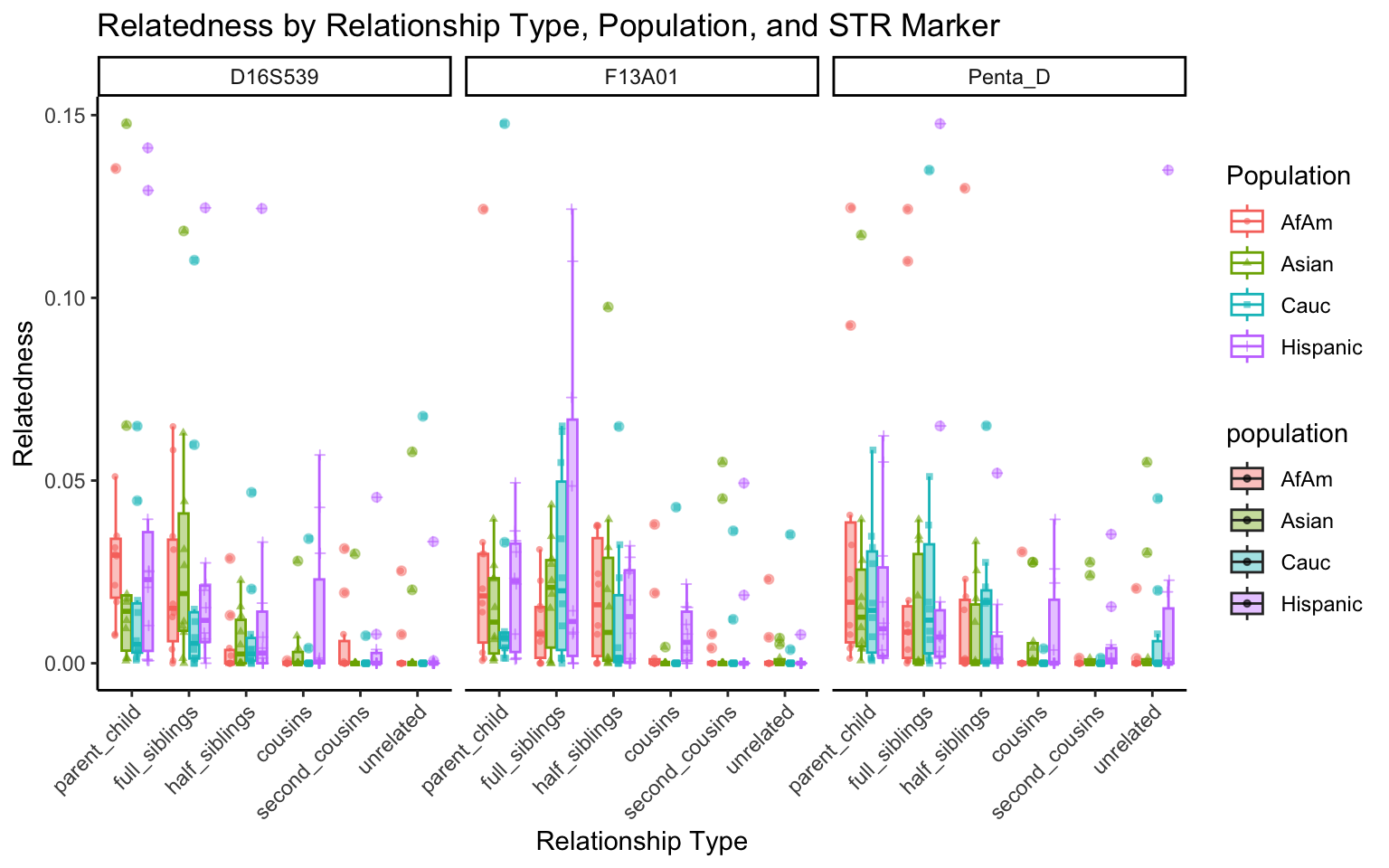
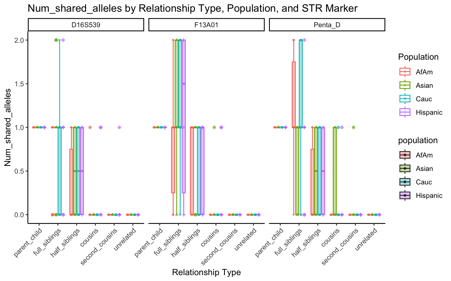
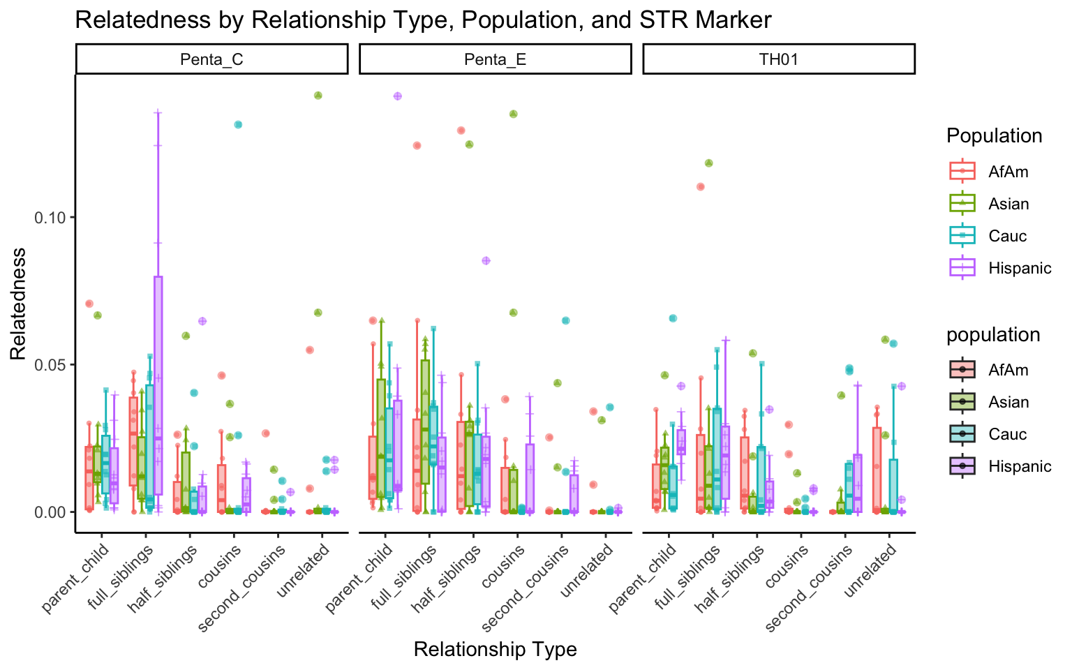
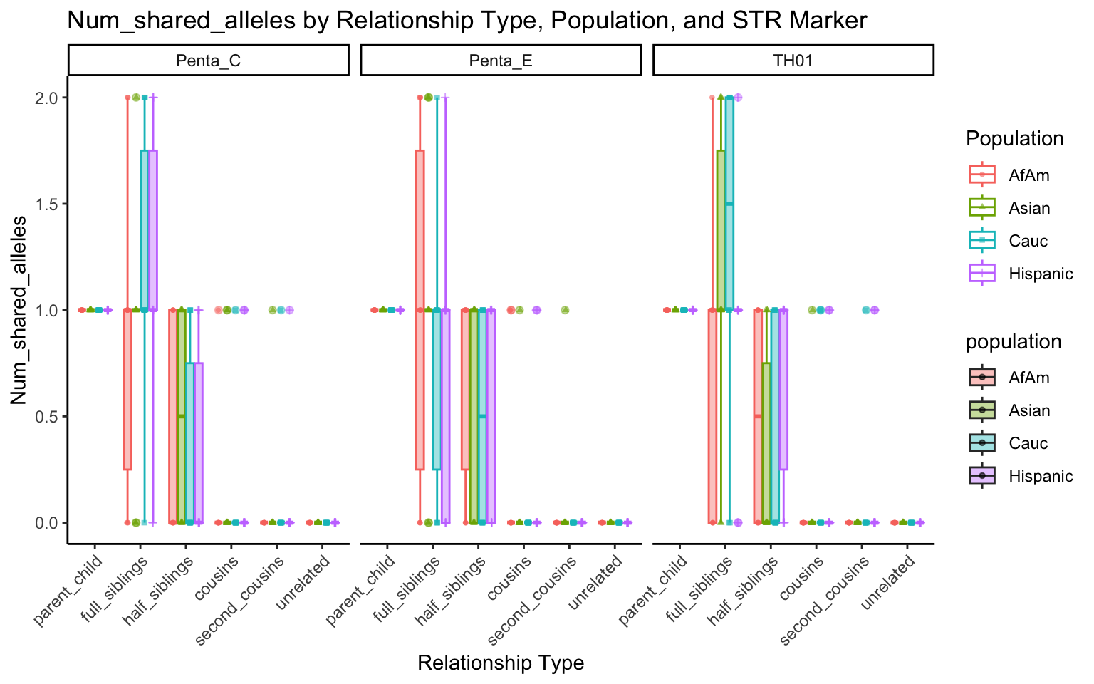
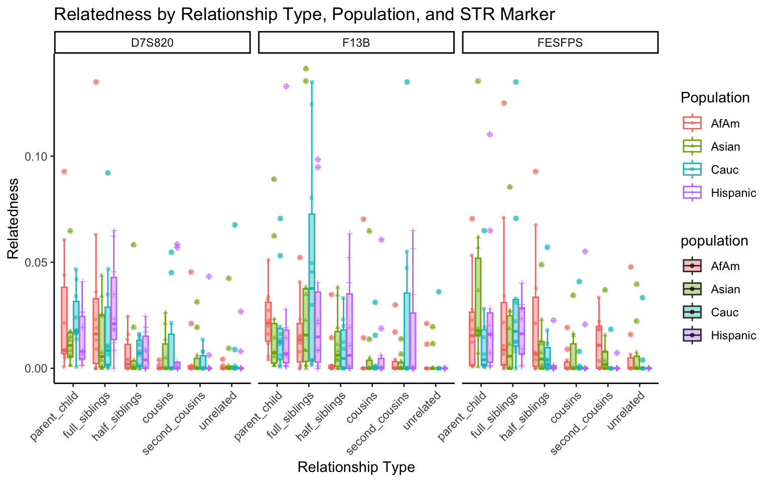
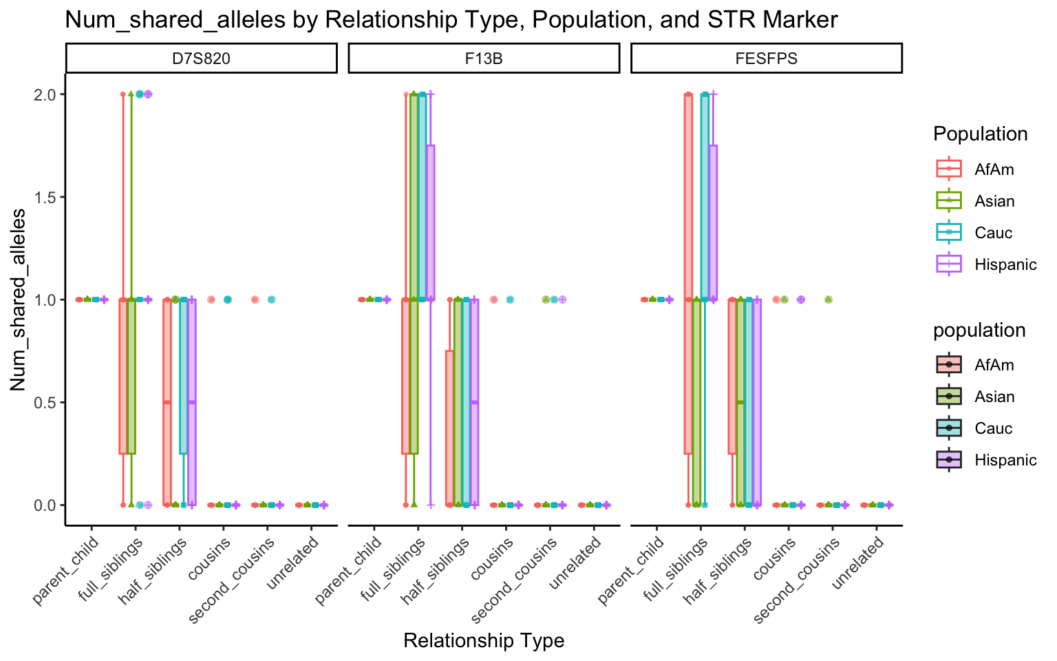
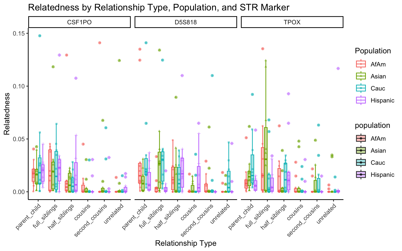
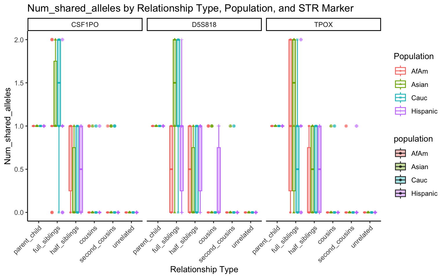
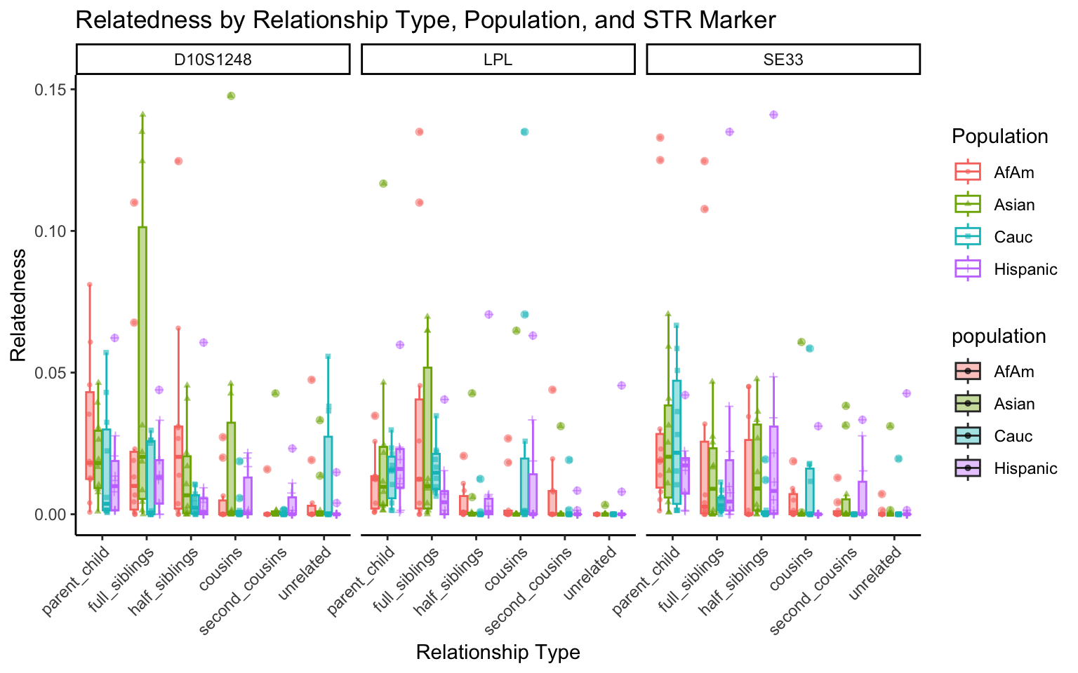
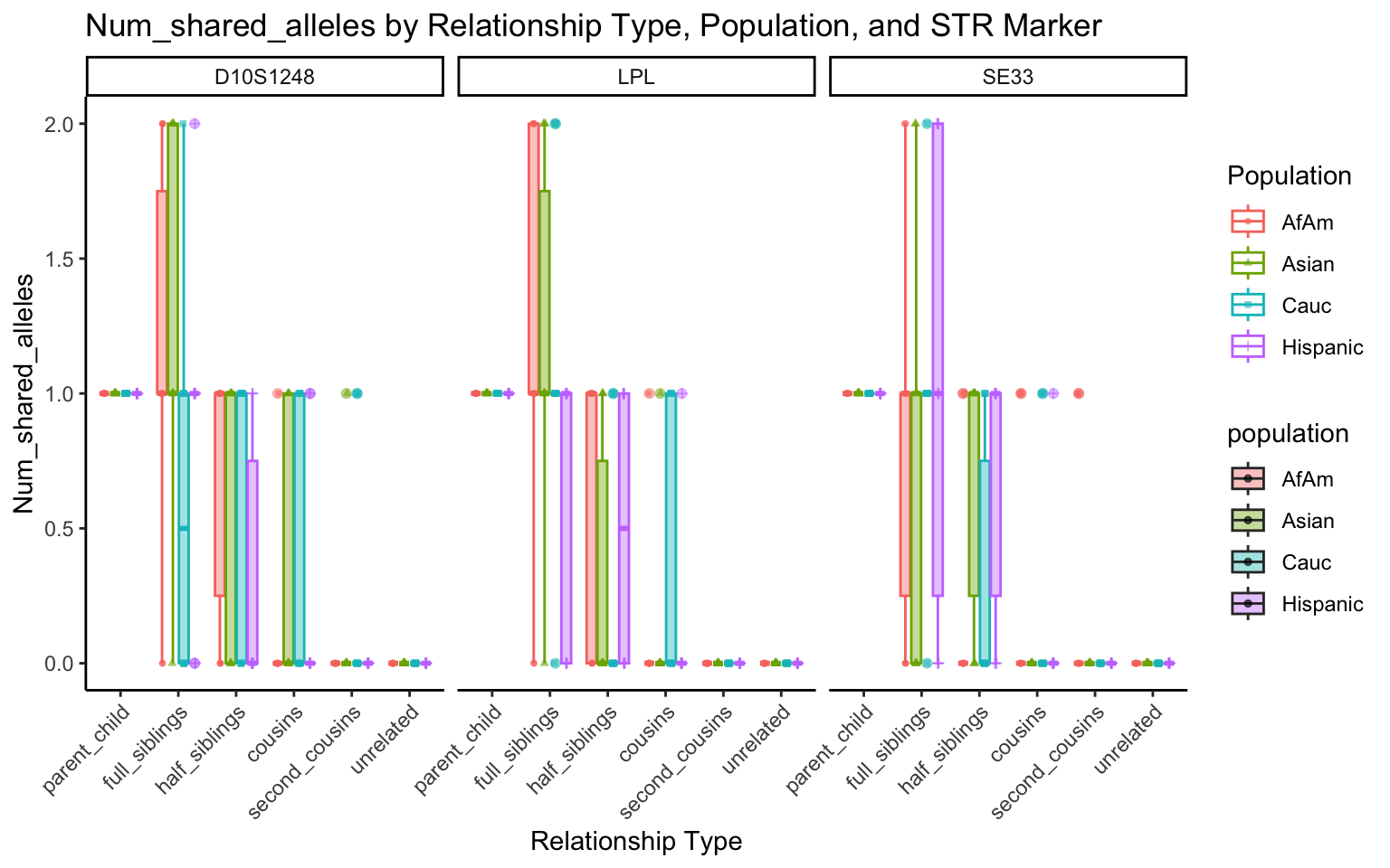
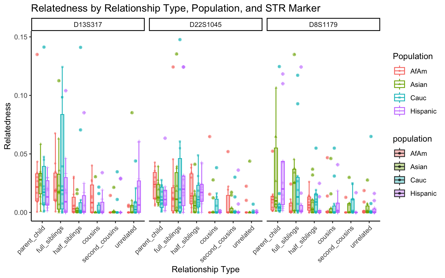
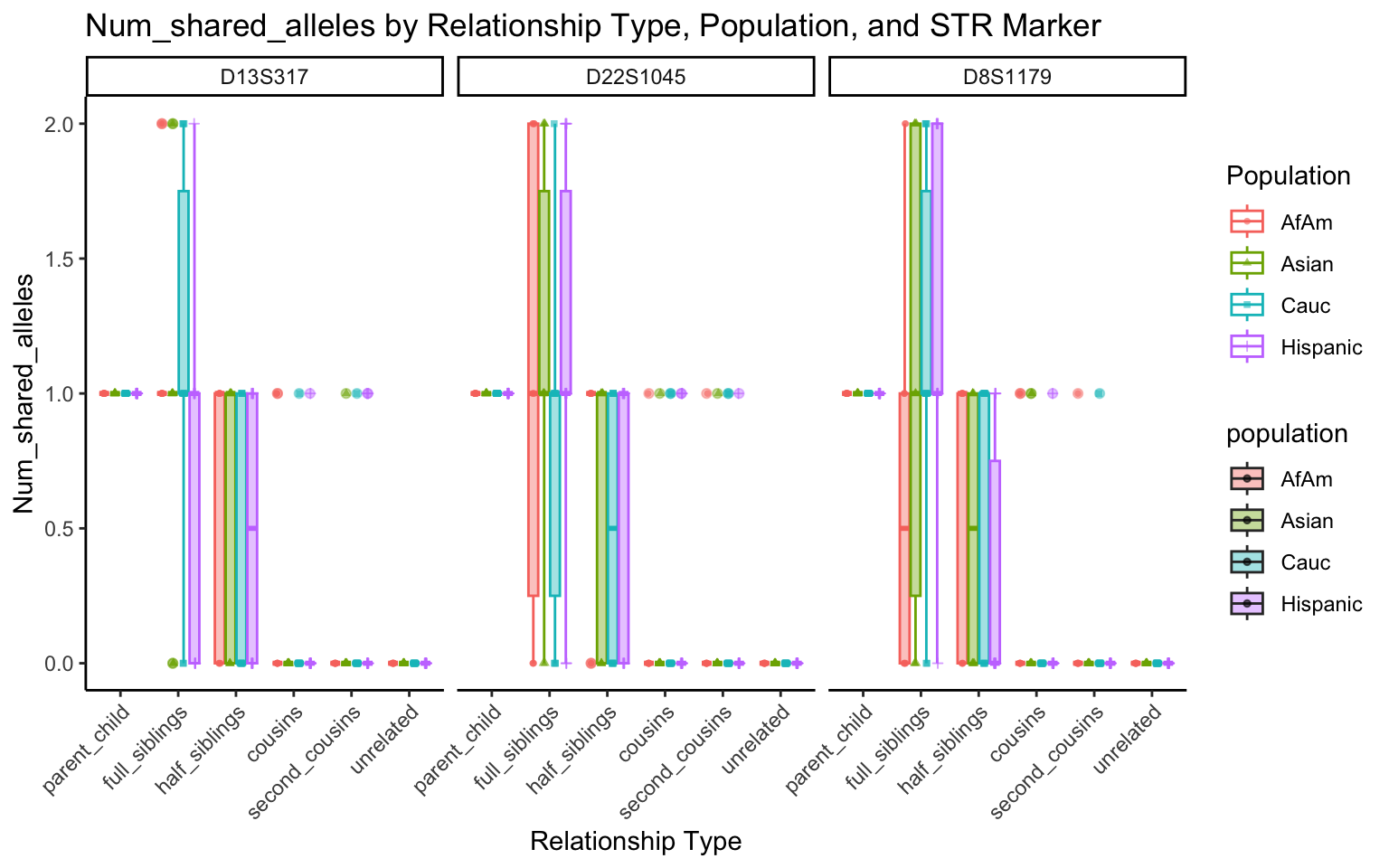
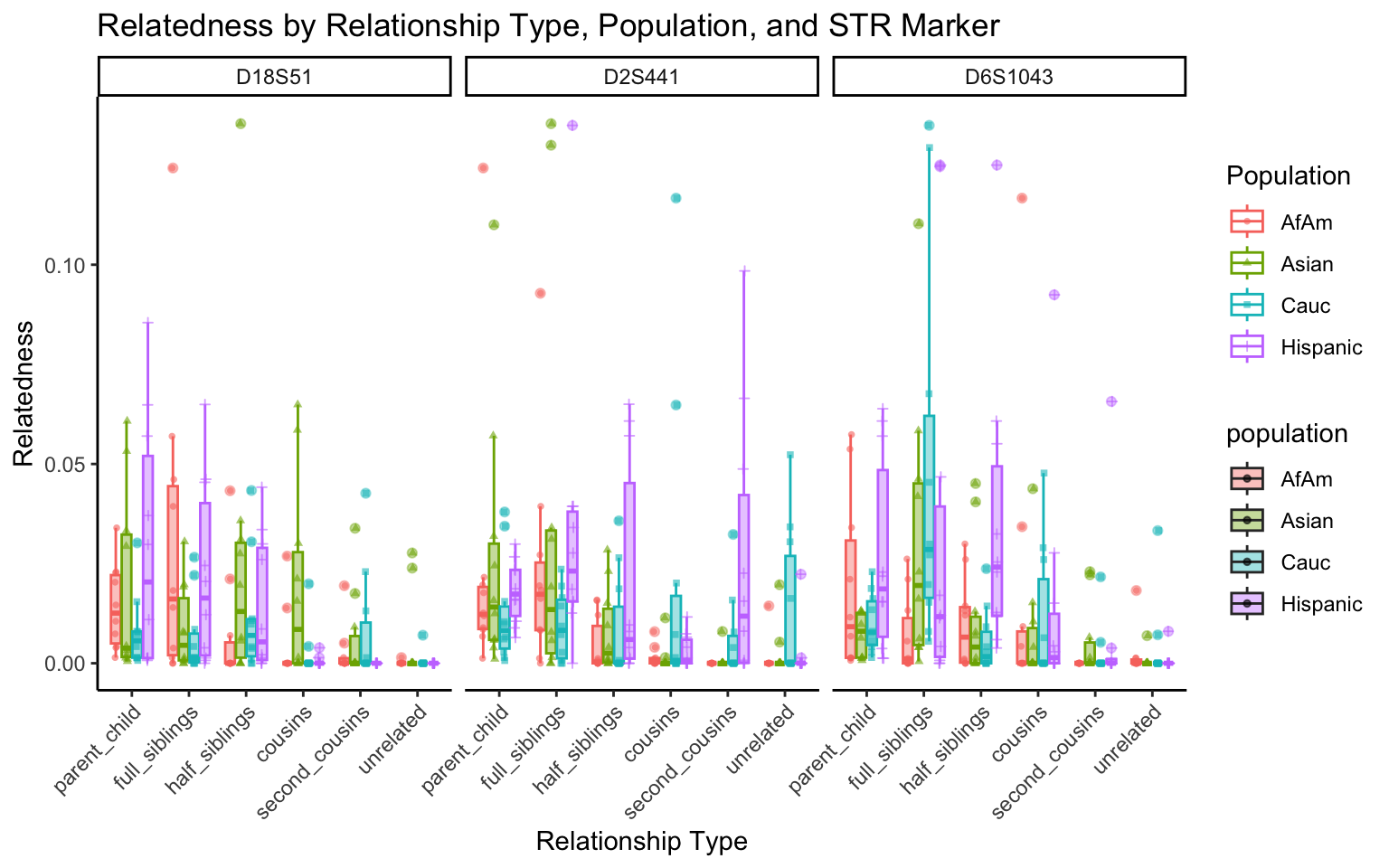
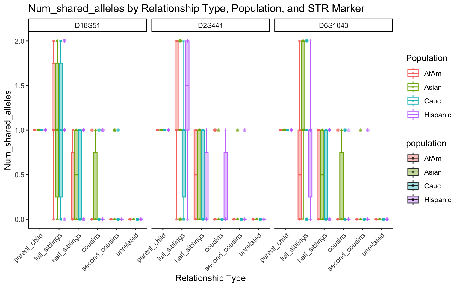
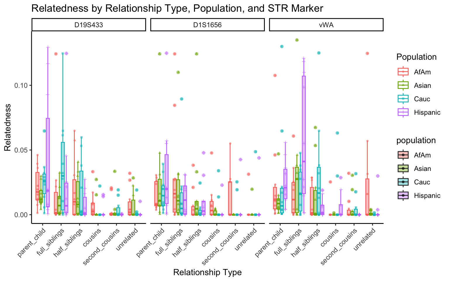
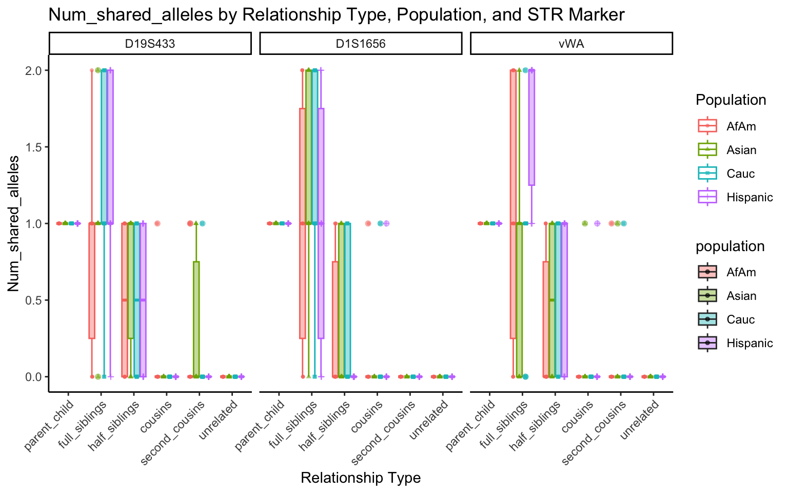
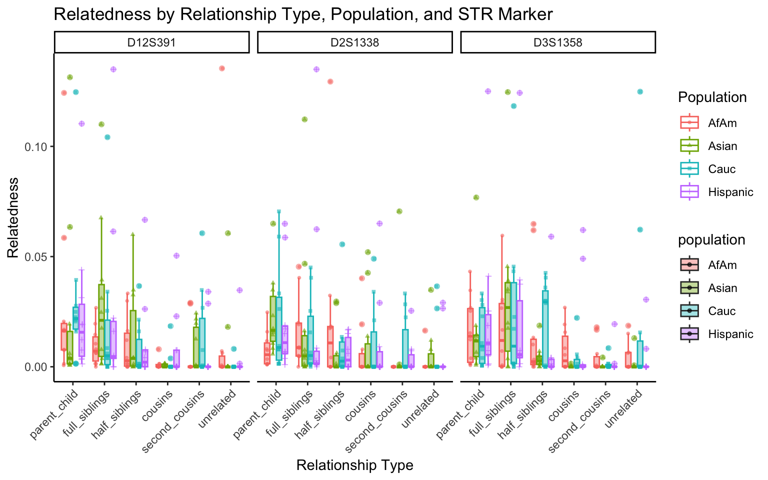
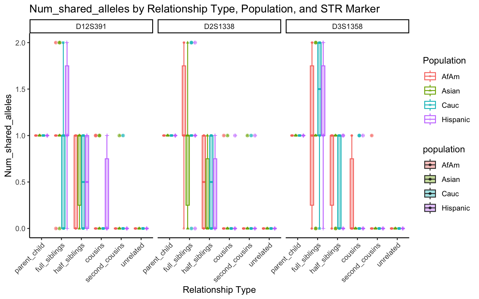
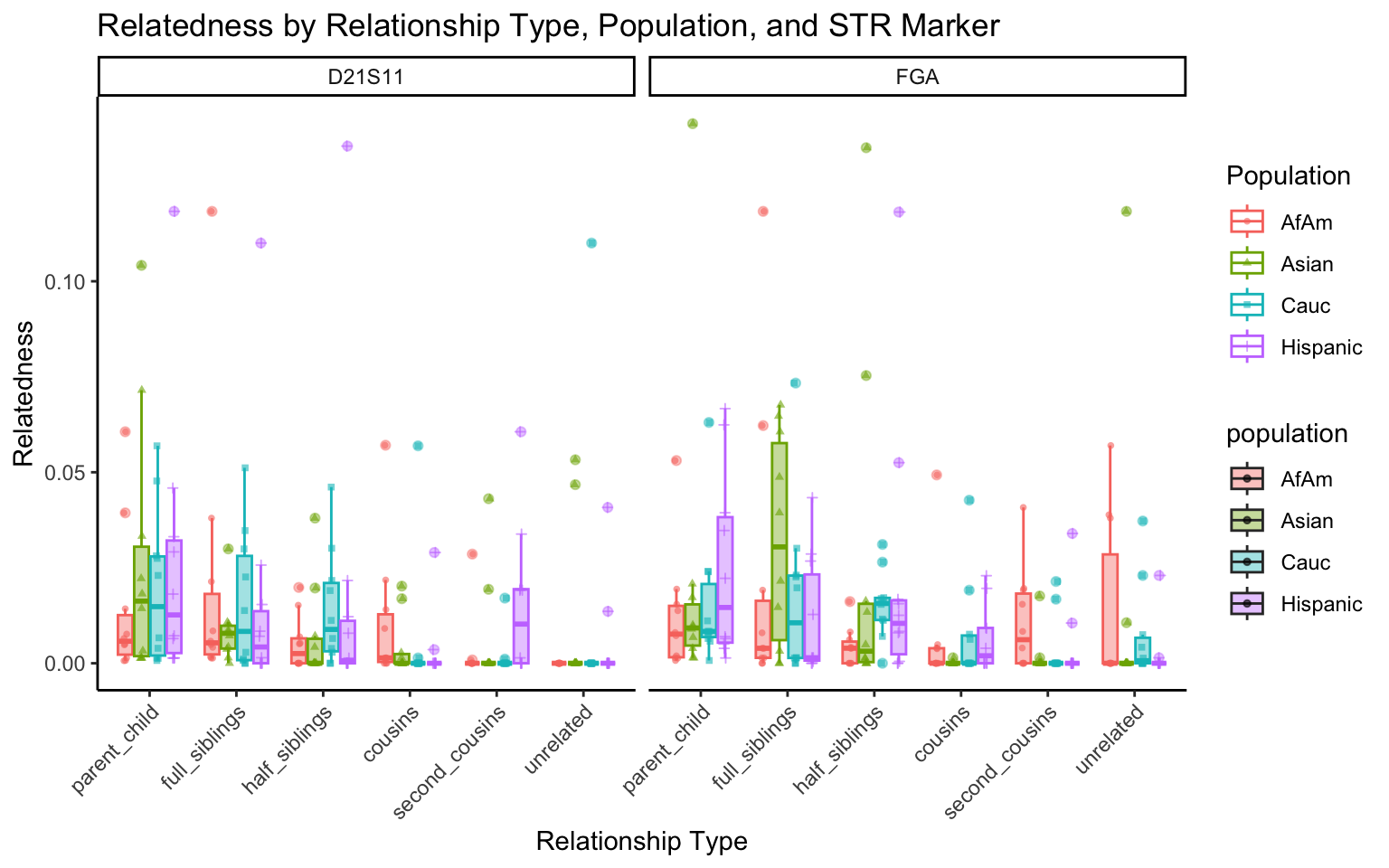
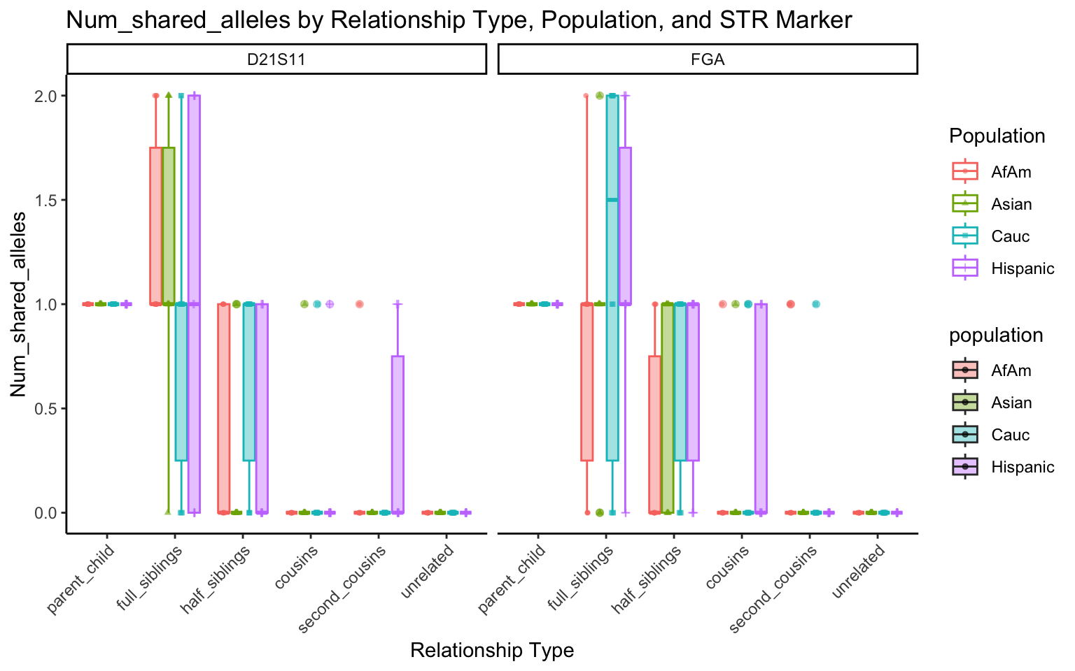
}create_plot <- function(df, variable_to_plot) {
# Create the plot
p <- ggplot(df, aes(x = relationship_type, y = .data[[variable_to_plot]], color = population, shape = population, fill = population)) +
geom_boxplot(alpha = 0.4) + # Change the order of geom_boxplot() and geom_point() and adjust alpha
geom_point(position = position_jitterdodge(jitter.width = 0.1, dodge.width = 0.75), size = 1, alpha = 0.6) +
facet_grid(. ~ marker) +
theme_classic() +
theme(axis.text.x = element_text(angle = 45, hjust = 1)) +
scale_x_discrete(limits = c('parent_child', 'full_siblings', 'half_siblings', 'cousins', 'second_cousins', 'unrelated')) +
labs(title = paste(ucfirst(variable_to_plot), "by Relationship Type, Population, and STR Marker"),
x = "Relationship Type",
y = ucfirst(variable_to_plot),
color = "Population",
shape = "Population")
return(p)
}# Filter your data for the first 3 unique STR markers
factor_vars <- c("marker", "population", "relationship_type")
numeric_vars <- c("relatedness", "num_shared_alleles")
# Filter your data for unique STR markers and remove the "all" population
results_df_filtered <- results_df %>%
filter(population != "all") %>%
mutate(
across(all_of(factor_vars), as.factor),
across(all_of(numeric_vars), as.numeric)
)
# Find the total number of unique markers
total_markers <- length(unique(results_df_filtered$marker))
# Iterate through the unique markers in groups of 3
for (i in seq(1, total_markers, by = 3)) {
# Filter the data for the current set of 3 or fewer markers
filtered_results_df <- results_df_filtered %>%
filter(marker %in% unique(marker)[i:min(i+2, total_markers)])
# Create and display the plots for the current set of markers
for (variable_to_plot in c("relatedness", "num_shared_alleles")) {
plot <- create_plot(df = filtered_results_df, variable_to_plot = variable_to_plot)
print(plot) # Print the plot to display it in the RMarkdown document
}
}
All Markers together
# Function to simulate genotypes for a pair of individuals
multi_simulate_genotypes <- function(allele_frequencies, relationship_type) {
  # Initialize an empty list to store results
  genotypes <- list()

  # Iterate over all markers
  for (marker in names(allele_frequencies)) {
    individual1 <- sample(names(allele_frequencies[[marker]]), size = 2, replace = TRUE, prob = allele_frequencies[[marker]])

    # Relationship probabilities
    relationship_probs <- list(
      'parent_child' = c(0, 1, 0),
      'full_siblings' = c(1/4, 1/2, 1/4),
      'half_siblings' = c(1/2, 1/2, 0),
      'cousins' = c(7/8, 1/8, 0),
      'second_cousins' = c(15/16, 1/16, 0),
      'unrelated' = c(1, 0, 0)
    )

    prob_shared_alleles <- relationship_probs[[relationship_type]]
    num_shared_alleles <- sample(c(0, 1, 2), size = 1, prob = prob_shared_alleles)
    individual2 <- c(sample(individual1, size = num_shared_alleles), sample(names(allele_frequencies[[marker]]), size = 2 - num_shared_alleles, replace = TRUE, prob = allele_frequencies[[marker]]))
    print(paste("The value of individual1 is:", individual1))
    print(paste("The value of individual2 is:", individual2))

    # Add the simulated genotypes to the list
    genotypes[[marker]] <- list(individual1 = individual1, individual2 = individual2, num_shared_alleles = num_shared_alleles)
  }

  # Return the list of simulated genotypes
  return(genotypes)
}

# Function to simulate genotypes and calculate relatedness for different relationships
multi_simulate_relatedness <- function(df, population, relationship_type) {
  # Filter the allele frequencies for the marker and population
  # allele_frequencies <- split(df[df$population == population, ], df$marker)
  allele_frequencies <- split(df[df$population == population, ]$frequency, df$marker)
  print(allele_frequencies)


  # Simulate genotypes
  simulated_genotypes <- multi_simulate_genotypes(allele_frequencies, relationship_type)

  # Calculate relatedness for each marker and store in a list
  relatedness_data <- lapply(names(simulated_genotypes), function(marker) {
    calculate_relatedness(simulated_genotypes[[marker]], allele_frequencies[[marker]])
  })

  # Convert the list of relatedness data to a dataframe
  relatedness_df <- do.call(rbind, lapply(relatedness_data, function(x) as.data.frame(t(unlist(x)))))

  # Add the marker, population, and relationship type to the dataframe
  relatedness_df$marker <- names(relatedness_data)
  relatedness_df$population <- population
  relatedness_df$relationship_type <- relationship_type

  return(relatedness_df)
}
# Function to simulate genotypes for a pair of individuals for all markers
simulate_genotypes_all_markers <- function(df, relationship_type, population) {
markers <- unique(df$marker)
# Simulate the first individual's alleles by drawing from the population frequency for each marker
individual1 <- setNames(lapply(markers, function(marker) {
allele_frequencies <- df %>%
filter(marker == marker, population == population) %>%
pull(frequency) %>%
setNames(df$allele)
sample(names(allele_frequencies), size = 2, replace = TRUE, prob = allele_frequencies)
}), markers)
# Relationship probabilities
relationship_probs <- list(
'parent_child' = c(0, 1, 0),
'full_siblings' = c(1/4, 1/2, 1/4),
'half_siblings' = c(1/2, 1/2, 0),
'cousins' = c(7/8, 1/8, 0),
'second_cousins' = c(15/16, 1/16, 0),
'unrelated' = c(1, 0, 0)
)
prob_shared_alleles <- relationship_probs[[relationship_type]]
num_shared_alleles <- sample(c(0, 1, 2), size = 1, prob = prob_shared_alleles)
individual2 <- setNames(lapply(markers, function(marker) {
allele_frequencies <- df %>%
filter(marker == marker, population == population) %>%
arrange(marker, allele) %>%
pull(frequency) %>%
setNames(df$allele)
prob_shared_alleles <- relationship_probs[[relationship_type]]
non_zero_indices <- which(prob_shared_alleles != 0)
num_shared_alleles <- sample(non_zero_indices - 1, size = 1, prob = prob_shared_alleles[non_zero_indices])
alleles_from_individual1 <- sample(individual1[[marker]], size = num_shared_alleles)
alleles_from_population <- sample(names(allele_frequencies), size = 2 - num_shared_alleles, replace = TRUE, prob = allele_frequencies)
return(c(alleles_from_individual1, alleles_from_population))
}), markers)
# Return the simulated genotypes
return(list(individual1 = individual1, individual2 = individual2))
}
# Function to calculate the index of relatedness for all markers
calculate_relatedness_all_markers <- function(simulated_genotypes, df, population) {
markers <- names(simulated_genotypes$individual1)
# Calculate the number of shared alleles for each marker
num_shared_alleles <- sapply(markers, function(marker) {
sum(simulated_genotypes$individual1[[marker]] %in% simulated_genotypes$individual2[[marker]])
})
# Calculate the index of relatedness as the number of shared alleles weighted inversely to their frequencies
# Now considering both individuals' alleles for the inverse frequency weighting
relatedness <- sapply(markers, function(marker) {
allele_frequencies <- df %>%
filter(marker == marker, population == population) %>%
pull(frequency) %>%
setNames(df$allele)
num_shared_alleles[marker] / (sum(1 / allele_frequencies[simulated_genotypes$individual1[[marker]]]) + sum(1 / allele_frequencies[simulated_genotypes$individual2[[marker]]]))
})
# Return the index of relatedness
return(list(relatedness = relatedness, num_shared_alleles = num_shared_alleles))
}
# Function to simulate genotypes and calculate relatedness for different relationships for all markers
simulate_relatedness_all_markers <- function(df, relationship_type, population) {
# Simulate genotypes for all markers
simulated_genotypes <- simulate_genotypes_all_markers(df, relationship_type, population)
# Calculate and return the relatedness for all markers
relatedness_data <- calculate_relatedness_all_markers(simulated_genotypes, df, population)
# Before returning the results_df, add marker and population information
results_df$marker <- rownames(results_df)
results_df$population <- population
return(relatedness_data)
}Visualizations
# Define the list of relationship types
relationship_types <- c('parent_child', 'full_siblings', 'half_siblings', 'cousins', 'second_cousins', 'unrelated')

# Create a dataframe of all combinations of populations and relationship types
combinations <- expand.grid(population = unique(df$population), relationship_type = relationship_types)

# Apply the function to each combination
results <- combinations %>%
  split(seq(nrow(.))) %>%
  map_dfr(function(combination) {
    population <- combination$population
    relationship_type <- combination$relationship_type
    # cat("Processing:", "population =", population, "; relationship_type =", relationship_type, "\n")
    sim_results <- simulate_relatedness_all_markers(df, relationship_type[[1]], population[[1]])

    # Bind resulting data frames
    tibble(
      population = population,
      relationship_type = relationship_type,
      sim_results = list(sim_results)
    )
  })

multi_results <- results %>%
  mutate(
    sum_relatedness = map_dbl(sim_results, function(x) {
      sum(x[["relatedness"]], na.rm = TRUE)
    }),
    sum_alleles = map_dbl(sim_results, function(x) {
      sum(x[["num_shared_alleles"]], na.rm = TRUE)
    })
  ) %>%
  select(-sim_results)

multi_results
# A tibble: 30 × 4
population relationship_type sum_relatedness sum_alleles
<fct> <fct> <dbl> <dbl>
1 AfAm parent_child 0.650 32
2 all parent_child 0.553 32
3 Asian parent_child 0.377 30
4 Cauc parent_child 0.449 36
5 Hispanic parent_child 0.462 33
6 AfAm full_siblings 0.488 25
7 all full_siblings 0.897 35
8 Asian full_siblings 0.679 31
9 Cauc full_siblings 0.738 32
10 Hispanic full_siblings 0.566 31
# ℹ 20 more rows# Define the number of simulations
n_sims <- 100
# Define the list of relationship types
relationship_types <- c('parent_child', 'full_siblings', 'half_siblings', 'cousins', 'second_cousins', 'unrelated')
# Create a dataframe of all combinations of populations, relationship types, and simulations
combinations <- expand.grid(population = unique(df$population), relationship_type = relationship_types, simulation = 1:n_sims)
# Apply the function to each combination
results <- combinations %>%
split(seq(nrow(.))) %>%
map_dfr(function(combination) {
population <- combination$population
relationship_type <- combination$relationship_type
sim <- combination$simulation
# cat("Processing:", "population =", population, "; relationship_type =", relationship_type, "; simulation =", sim, "\n")
sim_results <- simulate_relatedness_all_markers(df, relationship_type[[1]], population[[1]])
# Bind resulting data frames
tibble(
population = population,
relationship_type = relationship_type,
simulation = sim,
sim_results = list(sim_results)
)
})
multi_results <- results %>%
mutate(
sum_relatedness = map_dbl(sim_results, function(x) {
sum(x[["relatedness"]], na.rm = TRUE)
}),
sum_alleles = map_dbl(sim_results, function(x) {
sum(x[["num_shared_alleles"]], na.rm = TRUE)
})
) %>%
select(-sim_results)
multi_results# A tibble: 3,000 × 5
population relationship_type simulation sum_relatedness sum_alleles
<fct> <fct> <int> <dbl> <dbl>
1 AfAm parent_child 1 0.301 33
2 all parent_child 1 0.395 29
3 Asian parent_child 1 0.534 31
4 Cauc parent_child 1 0.393 30
5 Hispanic parent_child 1 0.453 35
6 AfAm full_siblings 1 0.776 35
7 all full_siblings 1 0.248 30
8 Asian full_siblings 1 0.656 32
9 Cauc full_siblings 1 0.363 30
10 Hispanic full_siblings 1 0.342 30
# ℹ 2,990 more rowscreate_plot <- function(df, variable_to_plot) {
# Create the plot
p <- ggplot(df, aes(x = relationship_type, y = .data[[variable_to_plot]], color = population, shape = population, fill = population)) +
geom_boxplot(alpha = 0.4, position = position_dodge(width = 0.75)) +
geom_point(position = position_jitterdodge(jitter.width = 0.1, dodge.width = 0.75), size = 1, alpha = 0.6) +
theme_classic() +
theme(axis.text.x = element_text(angle = 45, hjust = 1)) +
scale_x_discrete(limits = c('parent_child', 'full_siblings', 'half_siblings', 'cousins', 'second_cousins', 'unrelated')) +
labs(title = paste(ucfirst(variable_to_plot), "by Relationship Type and Population"),
x = "Relationship Type",
y = ucfirst(variable_to_plot),
color = "Population",
shape = "Population")
return(p)
}# Filter your data for unique STR markers and remove the "all" population
df_plt_multi_results <- multi_results %>%
filter(population != "all") %>%
select(-simulation)
p <- create_plot(df_plt_multi_results, "sum_relatedness")
p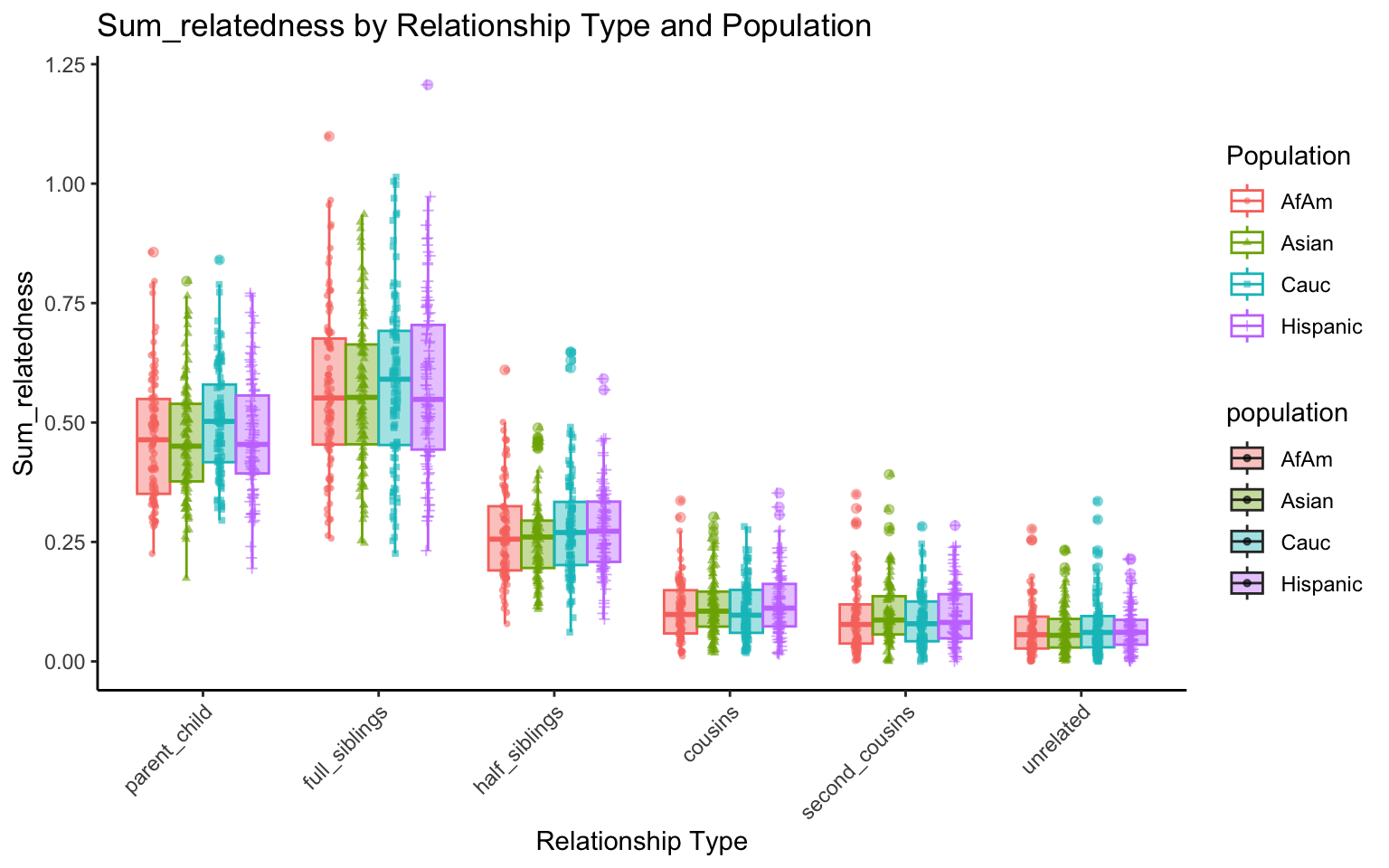
plt_allele <- create_plot(df_plt_multi_results, "sum_alleles")

plt_allele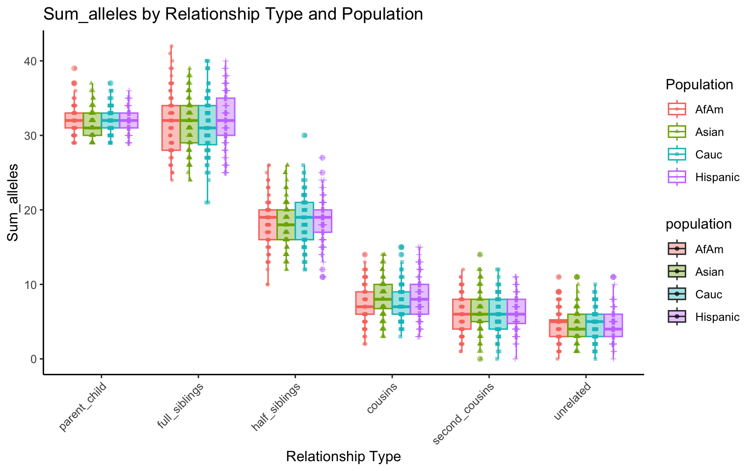
`
Probabilities
sessionInfo()R version 4.2.2 (2022-10-31)
Platform: aarch64-apple-darwin20 (64-bit)
Running under: macOS Ventura 13.3.1
Matrix products: default
BLAS: /Library/Frameworks/R.framework/Versions/4.2-arm64/Resources/lib/libRblas.0.dylib
LAPACK: /Library/Frameworks/R.framework/Versions/4.2-arm64/Resources/lib/libRlapack.dylib
locale:
[1] en_US.UTF-8/en_US.UTF-8/en_US.UTF-8/C/en_US.UTF-8/en_US.UTF-8
attached base packages:
[1] stats graphics grDevices utils datasets methods base
other attached packages:
[1] lubridate_1.9.2 forcats_1.0.0 stringr_1.5.0 dplyr_1.1.2
[5] purrr_1.0.1 readr_2.1.4 tidyr_1.3.0 tibble_3.2.1
[9] ggplot2_3.4.2 tidyverse_2.0.0 readxl_1.4.2 workflowr_1.7.0
loaded via a namespace (and not attached):
[1] Rcpp_1.0.10 getPass_0.2-2 ps_1.7.5 rprojroot_2.0.3
[5] digest_0.6.31 utf8_1.2.3 R6_2.5.1 cellranger_1.1.0
[9] evaluate_0.20 httr_1.4.5 highr_0.10 pillar_1.9.0
[13] rlang_1.1.0 rstudioapi_0.14 whisker_0.4.1 callr_3.7.3
[17] jquerylib_0.1.4 rmarkdown_2.21 labeling_0.4.2 bit_4.0.5
[21] munsell_0.5.0 compiler_4.2.2 httpuv_1.6.9 xfun_0.39
[25] pkgconfig_2.0.3 htmltools_0.5.5 tidyselect_1.2.0 fansi_1.0.4
[29] crayon_1.5.2 tzdb_0.3.0 withr_2.5.0 later_1.3.0
[33] grid_4.2.2 jsonlite_1.8.4 gtable_0.3.3 lifecycle_1.0.3
[37] git2r_0.32.0 magrittr_2.0.3 scales_1.2.1 cli_3.6.1
[41] stringi_1.7.12 vroom_1.6.1 cachem_1.0.7 farver_2.1.1
[45] fs_1.6.1 promises_1.2.0.1 bslib_0.4.2 generics_0.1.3
[49] vctrs_0.6.2 tools_4.2.2 bit64_4.0.5 glue_1.6.2
[53] hms_1.1.3 processx_3.8.1 parallel_4.2.2 fastmap_1.1.1
[57] yaml_2.3.7 timechange_0.2.0 colorspace_2.1-0 knitr_1.42
[61] sass_0.4.5