Sound Classification
Example

Toni Heittola
toni.heittola@tuni.fi

Introduction

This presentation goes through basic steps to build a CNN-based sound classifier.

Outline

• Dataset
• Cross-validation set
• Acoustic features
• Learning the acoustic model
• Testing the learned model
• Evaluation

Example application – Acoustic scene classification

The goal of acoustic scene classification is to classify a test recording into one of the predefined ten acoustic scene classes

Key tools used in this example:

• dcase_util – used to ease data handling, https://github.com/DCASE-REPO/dcase_util
• keras – neural network API for fast experimentation used on top of tensorflow machine learning framework
• scikit-learn – set of machine learning tools, here used to evaluate the system output

Dataset

TUT Urban Acoustic Scenes 2018 development dataset is used in this example:

• The dataset was used as a development dataset in acoustic scene classfication task (task1A) in the DCASE2018 Challenge
• Recordings from 10 scene classes, 6 large European cities
• 5-6 minute recordings around selected locations, which were split into 10 second audio segments
• 8640 segments in total

Dataset can be downloaded and accessed easily by using dataset handler class from dcase_util:

db = dcase_util.datasets.TUTUrbanAcousticScenes_2018_DevelopmentSet(
    data_path=dataset_storage_path
).initialize()

Audio file count : 8640
Scene class count: 10

Basic statistics of the dataset:

MetaDataContainer :: Class
Items                               : 8640 
Unique
  Files                             : 8640 
  Scene labels                      : 10 
  Event labels                      : 0 
  Tags                              : 0 
  Identifiers                       : 286 
  Datasets                          : 0 
  Source labels                     : 1 

Scene statistics
  Scene label             Count   Identifiers   
  --------------------   ------   -----------   
  airport                   864            22   
  bus                       864            36   
  metro                     864            29   
  metro_station             864            40   
  park                      864            25   
  public_square             864            24   
  shopping_mall             864            22   
  street_pedestrian         864            28   
  street_traffic            864            25   
  tram                      864            35   

Important aspects

• We need to be aware of the recording location of each segment
• Audio segments from the same location around the same time are highly correlated
• Unrealistic to be able to train the system and test it with material recorded in the same location only a few minutes apart
• The cross-validation set should take this into account to give realistic performance estimates

Cross-validation set

• Dataset is released with a single train/test-split
• We need also a validation set to follow system performance on unseen data during the training process
• Dataset class from dcase_util can be used to split the original training set into a new training set and validation set (70/30 split done according to recording locations)

Train/Test split bundled with the dataset

Scene label	Train set (items)	Test set (items)	Split percentage	Train (locations)	Test (locations)
airport	599	265	69	15	7
bus	622	242	71	26	10
metro	603	261	69	20	9
metro_station	605	259	70	28	12
park	622	242	71	18	7
public_square	648	216	75	18	6
shopping_mall	585	279	67	16	6
street_pedestrian	617	247	71	20	8
street_traffic	618	246	71	18	7
tram	603	261	69	24	11
Overall	6122	2518	70	203	83

Generating validation set

• During the training, we need a validation set to follow system performance on unseen data
• The validation set can be extracted from the training set while taking location identifiers into account
• Dataset class can be used to generate a validation set and a new training set:

training_files, validation_files = db.validation_split(
    validation_amount=0.3, # split target 30% 
    fold=1, # cross-validation fold id      
    # balance based on scenes and locations
    balancing_mode='identifier_two_level_hierarchy', 
    disable_progress_bar=True
)

train_meta = db.train(1).filter(file_list=training_files)
validation_meta = db.train(1).filter(file_list=validation_files)

Training items  : 4134
Validation items: 1988

Train / Validation statistics

Scene label	Train (locations)	Validation (locations)	Split percentage	Train set (items)	Validation set (items)	Split percentage
airport	9	6	40.0	411	188	31.4
bus	16	10	38.5	413	209	33.6
metro	13	7	35.0	422	181	30.0
metro_station	18	10	35.7	408	197	32.6
park	12	6	33.3	425	197	31.7
public_square	12	6	33.3	433	215	33.2
shopping_mall	10	6	37.5	360	225	38.5
street_pedestrian	13	7	35.0	422	195	31.6
street_traffic	12	6	33.3	425	193	31.2
tram	16	8	33.3	415	188	31.2
Overall	131	72	35.5	4134	1988	32.5

Features – log-mel energies

Feature extractor initialized with parameters and used to extract features:

# Load audio 
audio = dcase_util.containers.AudioContainer().load(
    filename=db.audio_files[0], mono=True
)

# Create feature extractor
mel_extractor = dcase_util.features.MelExtractor(
    n_mels=40, 
    win_length_seconds=0.04, 
    hop_length_seconds=0.02, 
    fs=audio.fs
)

# Extract features
mel_data = mel_extractor.extract(y=audio)

Feature matrix

mel_data shape (frequency, time):
 (40, 501)

Learning examples

1) Feature matrix

# Load audio
audio = dcase_util.containers.AudioContainer().load(
    filename=train_meta[0].filename, mono=True
)

# Extract log-mel energies
sequence_length = 500        # 10s / 0.02s = 500
mel_extractor = dcase_util.features.MelExtractor(
    n_mels=40, win_length_seconds=0.04, hop_length_seconds=0.02, fs=audio.fs
)

features = mel_extractor.extract(audio.data)[:,:sequence_length]

features shape (frequency, time):
 (40, 500)

2) Target vector (one-hot encoded vector)

# List of scene labels
scene_labels = db.scene_labels()               

# Empty target vector
target_vector = numpy.zeros(len(scene_labels))      

# Place one at correct position 
target_vector[scene_labels.index(train_meta[0].scene_label)] = 1

array([1., 0., 0., 0., 0., 0., 0., 0., 0., 0.])

target vector shape (classes, ):
 (10,)

Learning data

All learning data is collected into X_train and Y_train matrices:

X_train shape (sequence, frequence, time):
 (4134, 40, 500)
Y_train shape (sequence, classes):
 (4134, 10)

Matrix data:

Neural network structure

Neural network consists of two CNN blocks, the pooling layer, and the output layer.

Next, we create a neural network structure layer by layer.

Input layer:

input_layer = Input(
    shape=(feature_vector_length, sequence_length), 
    name='Input'
)

Reshaping layer to add channel axis into input data:

x = Reshape(
    target_shape=(feature_vector_length, sequence_length, 1), 
    name='Input_Reshape'
)(input_layer)

Output shape (sequence, frequency, time, channel):
 (None, 40, 500, 1)

Two convolutional layer groups consisting of:

1) Convolution to capture context and extract high-level features:
kernel 5x5 and filters 64

x = Conv2D(
    filters=64, 
    kernel_size=(5, 5), 
    activation='linear', 
    padding='same', 
    data_format='channels_last',
    name='Conv1'
)(x)

2) Batch normalization to enable higher learning rates

x = BatchNormalization(
    axis=-1, 
    name='Conv1_BatchNorm'
)(x)

3) Activation (ReLu) to introduce non-linearity

x = Activation(
    activation='relu', name='Conv1_Activation'
)(x)

4) Pooling (2D) to extract dominant features

x = MaxPooling2D(
    pool_size=(2, 4), name='Conv1_Pooling'
)(x)

5) Dropout to avoid overfitting

x = Dropout(
    rate=0.2, name='Conv1_DropOut'
)(x)

Output shape of CNN layer group 1 (sequence, frequency, time, feature):
 (None, 20, 125, 64)

Second convolutional layer group:

x = Conv2D(filters=64, kernel_size=(5, 5), activation='linear', padding='same', data_format='channels_last', name='Conv2')(x)
x = BatchNormalization(axis=-1, name='Conv2_BatchNorm')(x)
x = Activation(activation='relu', name='Conv2_Activation')(x)
x = MaxPooling2D(pool_size=(2, 2), name='Conv2_Pooling')(x)
x = Dropout(rate=0.2, name='Conv2_DropOut')(x)

Output shape of CNN layer group 2 (sequence, frequency, time, feature):
 (None, 10, 62, 64)

Global max pooling is applied to the output of the last convolutional layer group to summarize output into a single vector:

x = GlobalMaxPooling2D(
    data_format='channels_last', 
    name='GlobalPooling'
)(x)

Output shape (sequence, feature):
 (None, 64)

Output layer as fully-connected layer with a softmax activation:

output_layer = Dense(
    units=len(db.scene_labels()), 
    activation='softmax', 
    name='Output'
)(x)

Output shape (sequence, class):
 (None, 10)

Training

Key parameters:

• Loss – function used to measure the difference between target and prediction
  categorical_crossentropy
• Metric – evaluated for training and validation data during the learning process
  categorical_accuracy
• Optimizer – function used to update the model to minimize the loss
• Learning rate – how much model parameters are updated at each step
• Batch size – how many learning examples are processed before updating model parameters
• Epochs – how many times all learning data is gone through during the training procedure

model.compile(
    loss='categorical_crossentropy',
    metrics=['categorical_accuracy'],
    optimizer=keras.optimizers.Adam(learning_rate=0.001, decay=0.001)
)

# Track power consumption during the training
tracker = EmissionsTracker("Sound Classification Tutorial", output_dir=os.path.join('data', 'training_codecarbon'))
tracker.start()
# Track time
start_time = time.time()
# Start training process
history = model.fit(
    x=X_train, y=Y_train,
    validation_data=(X_validation, Y_validation),
    callbacks=callback_list,
    verbose=0,
    epochs=100,
    batch_size=16
)
# Stop tracking
stop_time = time.time()
tracker.stop()

  Training
            Loss                                Metric                             
            categorical_crossentropy            categorical_accuracy               
  Epoch     Train             Val               Train             Val              
  -------   ---------------   ---------------   ---------------   ---------------  
  1         1.5075            1.6670            0.4557            0.3602           
  2         1.3583            1.4756            0.4981            0.4542           
  3         1.2583            1.4834            0.5467            0.4814           
  4         1.1897            1.4104            0.5622            0.4306           
  5         1.1327            1.3432            0.5936            0.4628           
  6         1.0801            1.9897            0.6101            0.3099           
  7         1.0256            1.2844            0.6352            0.5231           
  8         0.9925            1.4193            0.6432            0.4527           
  9         0.9589            1.3612            0.6589            0.4899           
  10        0.9415            1.3491            0.6626            0.4643           
  11        0.9026            1.2894            0.6802            0.5040           
  12        0.8873            1.4195            0.6848            0.4437           
  13        0.8590            1.5074            0.6971            0.4366           
  14        0.8474            1.1322            0.6971            0.5568           
  15        0.8359            1.3068            0.7042            0.5367           
  16        0.8178            1.2733            0.7083            0.5392           
  17        0.7952            1.1023            0.7170            0.5805           
  18        0.7781            1.2346            0.7339            0.5161           
  19        0.7725            1.0566            0.7308            0.5850           
  20        0.7717            1.3855            0.7281            0.5065           
  21        0.7492            1.1186            0.7472            0.5830           
  22        0.7438            1.1939            0.7436            0.5418           
  23        0.7258            1.0572            0.7511            0.5946           
  24        0.7284            1.0736            0.7446            0.5800           
  25        0.7125            1.0651            0.7559            0.5805           
  26        0.7073            1.1462            0.7535            0.5629           
  27        0.7035            1.3761            0.7574            0.4764           
  28        0.6953            1.1581            0.7511            0.5392           
  29        0.6875            1.0682            0.7651            0.5936           
  30        0.6741            1.0484            0.7721            0.6056           
  31        0.6759            1.3890            0.7683            0.5020           
  32        0.6818            1.1066            0.7663            0.5830           

Training history

Testing stage

Extract features for test item:

# Get test item
item = db.test(fold=1)[0]

# Extract features
features = mel_extractor.extract(
    AudioContainer().load(filename=item.filename, mono=True)
)[:,:sequence_length]

Reshape the matrix to match the model input:

input_data = numpy.expand_dims(features, 0)

Feed input data into the model to get probabilities for each scene class:

probabilities = model.predict(x=input_data)

Classify by selecting the class giving maximum output:

frame_decisions = dcase_util.data.ProbabilityEncoder().binarization(
    probabilities=probabilities.T,
    binarization_type='frame_max'
).T  

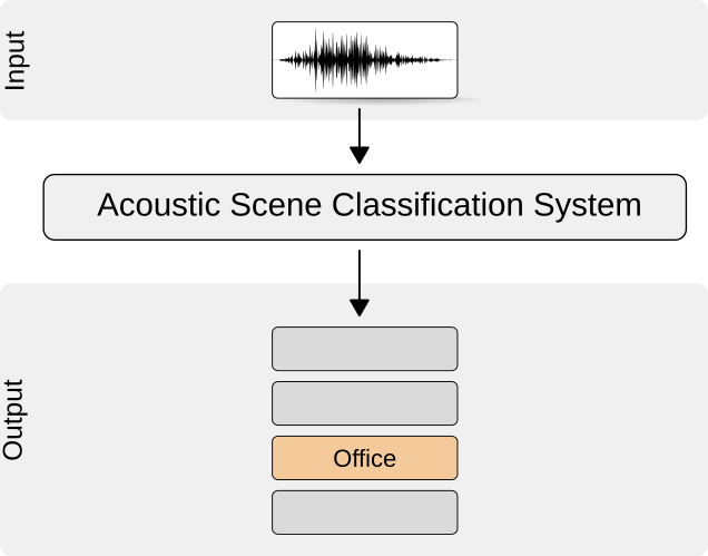
Scene label:

Evaluation

import sklearn

# Get confusion matrix with counts
confusion_matrix = sklearn.metrics.confusion_matrix(y_true, y_pred)

# Transform matrix into percentages, normalize row-wise
conf = confusion_matrix * 100.0 / confusion_matrix.sum(axis=1)[:, numpy.newaxis]  

# Fetch class-wise accuracies from diagonal
class_wise_accuracies = numpy.diag(conf)                

# Calculate overall accuracy
macro_averaged_accuracy = numpy.mean(class_wise_accuracies)

Macro-averaged accuracy: 61.6 %

Class-wise accuracies

Scene label	Accuracy
airport	69.1
bus	56.2
metro	62.5
metro_station	35.5
park	85.5
public_square	53.2
shopping_mall	64.5
street_pedestrian	44.5
street_traffic	81.3
tram	64.0
Average	61.6

Confusion matrix

How to improve:

• Collect more material
• Use data augmentation to generate more variability in learning examples
• Use transfer learning techniques to distill knowledge from other tasks
• Use different network architectures