GPSM
Troy Rowan
2020-09-20
Last updated: 2020-10-12
Checks: 7 0
Knit directory: local_adaptation_sequence/
This reproducible R Markdown analysis was created with workflowr (version 1.6.2). The Checks tab describes the reproducibility checks that were applied when the results were created. The Past versions tab lists the development history.
Great! Since the R Markdown file has been committed to the Git repository, you know the exact version of the code that produced these results.
Great job! The global environment was empty. Objects defined in the global environment can affect the analysis in your R Markdown file in unknown ways. For reproduciblity it’s best to always run the code in an empty environment.
The command set.seed(20200709) was run prior to running the code in the R Markdown file. Setting a seed ensures that any results that rely on randomness, e.g. subsampling or permutations, are reproducible.
Great job! Recording the operating system, R version, and package versions is critical for reproducibility.
Nice! There were no cached chunks for this analysis, so you can be confident that you successfully produced the results during this run.
Great job! Using relative paths to the files within your workflowr project makes it easier to run your code on other machines.
Great! You are using Git for version control. Tracking code development and connecting the code version to the results is critical for reproducibility.
The results in this page were generated with repository version 50ddc20. See the Past versions tab to see a history of the changes made to the R Markdown and HTML files.
Note that you need to be careful to ensure that all relevant files for the analysis have been committed to Git prior to generating the results (you can use wflow_publish or wflow_git_commit). workflowr only checks the R Markdown file, but you know if there are other scripts or data files that it depends on. Below is the status of the Git repository when the results were generated:
Ignored files:
    Ignored:    .Rhistory
    Ignored:    .Rproj.user/
    Ignored:    analysis/genes.txt
    Ignored:    code/commands.txt
    Ignored:    data/1KBulls_ids.txt
    Ignored:    data/200907_SIM/
    Ignored:    data/200910_RAN/
    Ignored:    data/Bos_taurus.ARS-UCD1.2.101.gtf.gz
    Ignored:    data/Bos_taurus.ARS-UCD1.2.QTL.gff.gz
    Ignored:    data/Johnston_ATAC-seq/
    Ignored:    data/animal_table.rds
    Ignored:    data/bovine_demo.sample_metadata.csv
    Ignored:    data/prism_climate_data/
    Ignored:    data/prism_dataframe.csv
    Ignored:    data/uszips.csv
    Ignored:    desktop.ini
    Ignored:    output/200822_Lab_IDs.csv
    Ignored:    output/200907_Lab_IDs.csv
    Ignored:    output/200909_RAN_Lab_IDs.csv
    Ignored:    output/200910_RAN/200910_RAN.phenotypes.csv
    Ignored:    output/200910_RAN/200910_RAN.phenotypes.txt
    Ignored:    output/200910_RAN/200910_RAN_Lab_IDs.csv
    Ignored:    output/200910_RAN/gpsm/
    Ignored:    output/200910_RAN/gwas/
    Ignored:    output/200910_RAN/phenotypes/200910_RAN.generation_proxy.txt
    Ignored:    output/200910_RAN/phenotypes/200910_RAN.info.csv
    Ignored:    output/200910_RAN/phenotypes/200910_RAN.noLSF.allenv.txt
    Ignored:    output/200910_RAN/phenotypes/200910_RAN.phenotyped_ids.txt
    Ignored:    output/200910_RAN/phenotypes/200910_RAN.regions.txt
    Ignored:    output/200910_RAN/subsets/
    Ignored:    output/200910_RAN_Lab_IDs.csv
    Ignored:    output/coresnps.50K.refaltaltref.txt
    Ignored:    output/coresnps.50K.txt
    Ignored:    output/coresnps.850K.refaltaltref.txt
    Ignored:    output/desktop.ini
    Ignored:    output/k10.allvars.seed2.rds
    Ignored:    output/k9.allvars.seed1.rds
    Ignored:    output/k9.allvars.seed2.rds
    Ignored:    output/k9.threevars.seed1.rds
    Ignored:    output/k9.threevars.seed2.rds
    Ignored:    output/kmeans_plotlist.RDS
    Ignored:    output/zipcode_zones.csv

Untracked files:
    Untracked:  analysis/Region_FST.Rmd
    Untracked:  analysis/selection_scans.Rmd
    Untracked:  code/GCTA_functions.R
    Untracked:  code/cluster/selscan.cluster.json
    Untracked:  code/cluster/sfs_selection.cluster.json
    Untracked:  code/config/200910_RAN.GPSM.config.yaml
    Untracked:  code/countgens_RAN.R
    Untracked:  code/snakemake_files/BOLT.snakefile
    Untracked:  code/snakemake_files/sfs_selection.snakefile
    Untracked:  ftpconfigs/
    Untracked:  functions.R
    Untracked:  output/200907_SIM.850K.bim
    Untracked:  output/200907_SIM/
    Untracked:  output/200910_RAN/fst/
    Untracked:  output/200910_RAN/greml/
    Untracked:  output/200910_RAN/selscan/
    Untracked:  test.Rmd
    Untracked:  test.html

Unstaged changes:
    Modified:   .gitignore
    Modified:   analysis/200910_RAN.envGWAS_results.Rmd
    Modified:   analysis/animal_locations.Rmd
    Modified:   analysis/phenotype_exploration.Rmd
    Modified:   code/annotation_functions.R
    Modified:   code/cluster/GCTA.cluster.json
    Modified:   code/config/200907_SIM.GPSM.config.yaml
    Modified:   code/config/200907_SIM.envGWAS.config.yaml
    Modified:   code/config/200910_RAN.config.yaml
    Modified:   code/config/200910_RAN_noLSF.config.yaml
    Modified:   code/snakemake_files/GCTA.snakefile
    Modified:   code/snakemake_files/selscan.snakefile
    Deleted:    data/README.md
    Modified:   output/200910_RAN/phenotypes/200910_RAN.age.txt
    Modified:   output/200910_RAN/phenotypes/200910_RAN.environment.txt
    Modified:   output/200910_RAN/phenotypes/200910_RAN.sex.txt
Note that any generated files, e.g. HTML, png, CSS, etc., are not included in this status report because it is ok for generated content to have uncommitted changes.
These are the previous versions of the repository in which changes were made to the R Markdown (analysis/GPSM.Rmd) and HTML (docs/GPSM.html) files. If you’ve configured a remote Git repository (see ?wflow_git_remote), click on the hyperlinks in the table below to view the files as they were in that past version.
| File | Version | Author | Date | Message |
|---|---|---|---|---|
| Rmd | 50ddc20 | Troy Rowan | 2020-10-12 | Updated GPSM with GREML estimates and manhattan plots |
| Rmd | f01e8ba | Troy Rowan | 2020-09-29 | RMarkdown updates that haven’t been pushed by workflowr |
simmental = read_csv("output/200907_SIM/phenotypes/200907_SIM.info.csv")
redangus = read_csv("output/200910_RAN/phenotypes/200910_RAN.info.csv")
Core SNP edits for BOLT-LMM These core “GRM” SNPs are used to control for structure in the population if we need to use BOLT-LMM
Red Angus GPSM Analysis
REML variance component estimates
Raw Age
Raw Age (n= 46,454):
| Source | Variance | SE |
|---|---|---|
| V(G) | 5.244 | 0.128 |
| V(e) | 4.789 | 0.040 |
| V(p) | 10.03 | 0.118 |
| V(G)/Vp | 0.523 | 0.007 |
Square Root
Square Root Transformed Age (n= 46,454):
| Source | Variance | SE |
|---|---|---|
| V(G) | 0.242 | 0.005 |
| V(e) | 0.151 | 0.001 |
| V(p) | 0.393 | 0.005 |
| V(G)/Vp | 0.616 | 0.006 |
Cube Root
Cube Root Transformed Age (n= 46,454):
| Source | Variance | SE |
|---|---|---|
| V(G) | 0.065 | 0.001 |
| V(e) | 0.037 | 0.000 |
| V(p) | 0.101 | 0.001 |
| V(G)/Vp | 0.637 | 0.006 |
Box-Cox
Box-Cox Transformed Age (n= 46,454):
| Source | Variance | SE |
|---|---|---|
| V(G) | 0.115 | 0.002 |
| V(e) | 0.060 | 0.001 |
| V(p) | 0.175 | 0.002 |
| V(G)/Vp | 0.657 | 0.006 |
Log
Log Transformed Age (n= 46,454):
| Source | Variance | SE |
|---|---|---|
| V(G) | 0.222 | 0.005 |
| V(e) | 0.115 | 0.001 |
| V(p) | 0.337 | 0.005 |
| V(G)/Vp | 0.657 | 0.006 |
Individual Residuals and Breeding Values
These are REML estimates of individual’s breeding values and residuals from GCTA GREML analysis
Age
plot_grid(
  read_blp("output/200910_RAN/greml/200910_RAN.age.850K.indi.blp") %>%
    left_join(redangus %>%
                select(international_id, age)) %>%
    ggplot(aes(sample = Residual))+
    stat_qq()+
    stat_qq_line(color = "red")+
    ggtitle("Raw Age GPSM\nResiduals")+
    theme_cowplot(),
  read_blp("output/200910_RAN/greml/200910_RAN.age.850K.indi.blp") %>%
    left_join(redangus %>%
                select(international_id, age)) %>%
    ggplot(aes(sample = BV))+
    stat_qq()+
    stat_qq_line(color = "red")+
    ggtitle("\nBreeding Values")+
    theme_cowplot())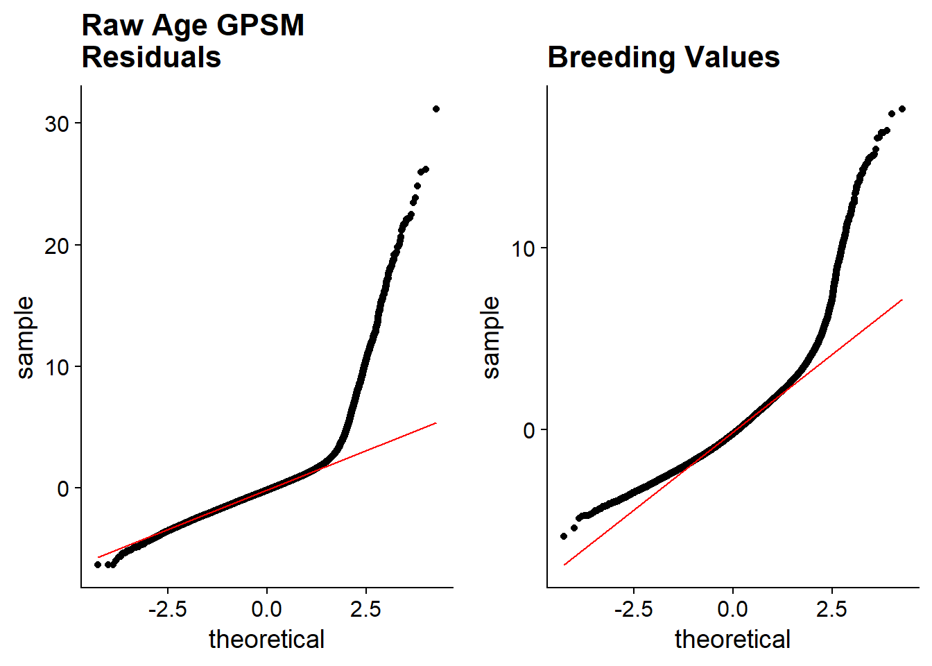
Square Root
plot_grid(
  read_blp("output/200910_RAN/greml/200910_RAN.sqrt_age.850K.indi.blp") %>%
    left_join(redangus %>%
                select(international_id, age)) %>%
    ggplot(aes(sample = Residual))+
    stat_qq()+
    stat_qq_line(color = "red")+
    ggtitle("Square Root Transformed Age \nGPSM Residuals")+
    theme_cowplot(),
  read_blp("output/200910_RAN/greml/200910_RAN.sqrt_age.850K.indi.blp") %>%
  left_join(redangus %>%
              select(international_id, age)) %>%
  ggplot(aes(sample = BV))+
  stat_qq()+
  stat_qq_line(color = "red")+
  ggtitle("\nBreeding Values")+
  theme_cowplot())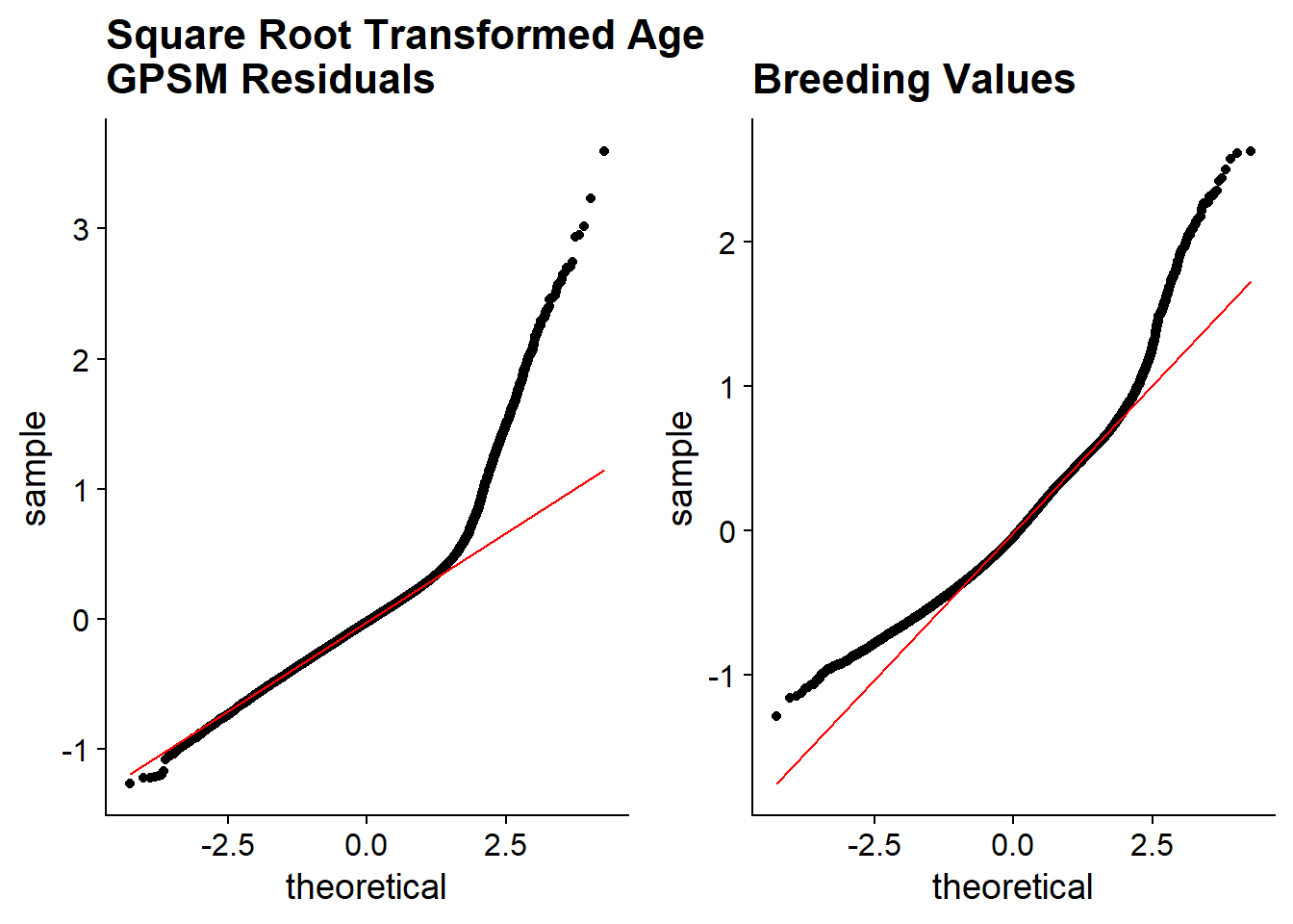
Cube Root
plot_grid(
  read_blp("output/200910_RAN/greml/200910_RAN.cbrt_age.850K.indi.blp") %>%
    left_join(redangus %>%
                select(international_id, age)) %>%
    ggplot(aes(sample = Residual))+
    stat_qq()+
    stat_qq_line(color = "red")+
    ggtitle("Cube Root Transformed Age \nGPSM Residuals")+
    theme_cowplot(),
  read_blp("output/200910_RAN/greml/200910_RAN.cbrt_age.850K.indi.blp") %>%
  left_join(redangus %>%
              select(international_id, age)) %>%
  ggplot(aes(sample = BV))+
  stat_qq()+
  stat_qq_line(color = "red")+
  ggtitle("\nGPSM Breeding Values")+
  theme_cowplot())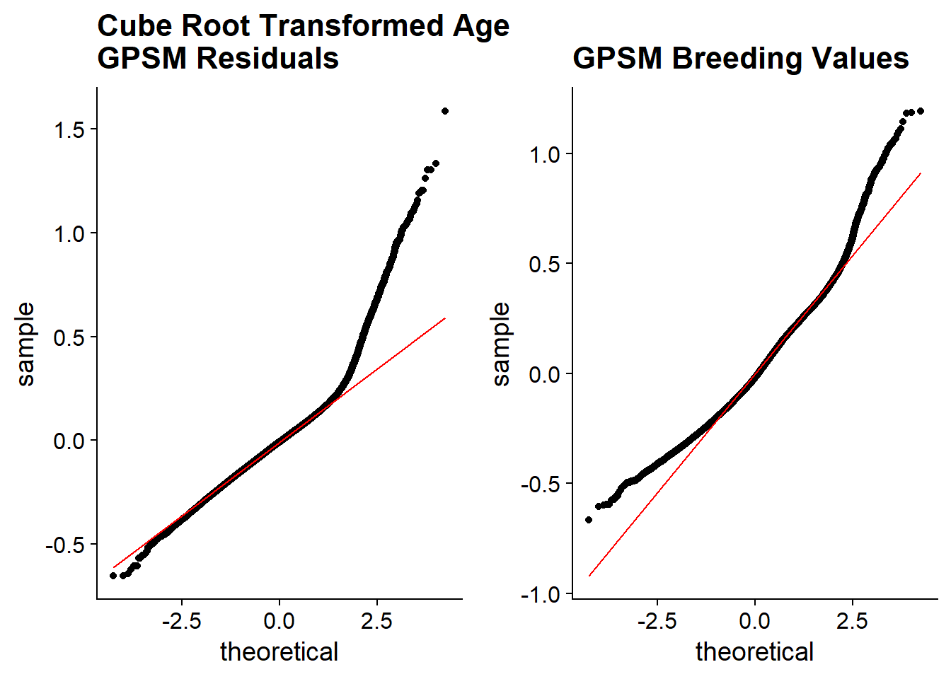
Box-Cox
plot_grid(
  read_blp("output/200910_RAN/greml/200910_RAN.bc_age.850K.indi.blp") %>%
    left_join(redangus %>%
                select(international_id, age)) %>%
    ggplot(aes(sample = Residual))+
    stat_qq()+
    stat_qq_line(color = "red")+
    ggtitle("Box-Cox Transformed Age \nGPSM Residuals")+
    theme_cowplot(),
  read_blp("output/200910_RAN/greml/200910_RAN.bc_age.850K.indi.blp") %>%
    left_join(redangus %>%
                select(international_id, age)) %>%
    ggplot(aes(sample = BV))+
    stat_qq()+
    stat_qq_line(color = "red")+
    ggtitle("\nGPSM Residuals")+
    theme_cowplot())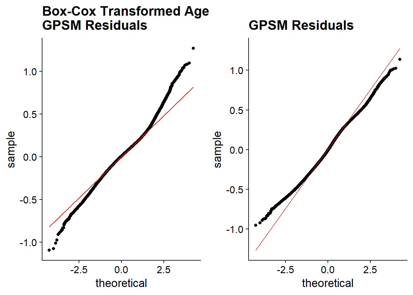
Log
plot_grid(read_blp("output/200910_RAN/greml/200910_RAN.log_age.850K.indi.blp") %>%
    left_join(redangus %>%
                select(international_id, age)) %>%
    ggplot(aes(sample = Residual))+
    stat_qq()+
    stat_qq_line(color = "red")+
    ggtitle("Log Transformed Age \nGPSM Residuals")+
    theme_cowplot(),
  read_blp("output/200910_RAN/greml/200910_RAN.log_age.850K.indi.blp") %>%
    left_join(redangus %>%
                select(international_id, age)) %>%
    ggplot(aes(sample = BV))+
    stat_qq()+
    stat_qq_line(color = "red")+
    ggtitle("\nGPSM Breeding Values")+
    theme_cowplot())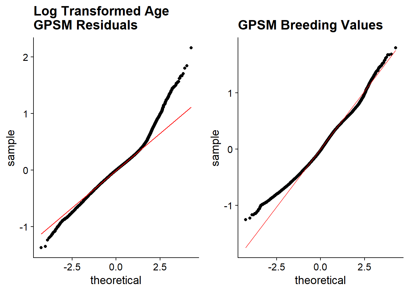
n(SigSNPs)
The number of significant SNPs in each analysis at various significance level cutoffs for both p and q values
| p<1e-5 | p<1e7.55e-7 | q<0.1 | q<0.05 | |
|---|---|---|---|---|
| Raw | 315 | 214 | 509 | 398 |
| Sqrt | 453 | 333 | 729 | 559 |
| Cbrt | 471 | 357 | 817 | 596 |
| BoxCox | 540 | 390 | 907 | 754 |
| Log | 513 | 377 | 822 | 715 |
GPSM GWAS Manhattan Plots for Transformed Age
Raw Age
(Significance threshold - Bonferroni)
plot_grid(
  ggmanhattan2(ran_gpsm_age,
               prune = 0.1,
               sig_threshold_p = 7.546167e-07),
  ggmanhattan2(ran_gpsm_age,
               prune = 0.1,
               sig_threshold_p = 7.546167e-07)+
    ylim(c(0,15)),
  nrow = 2)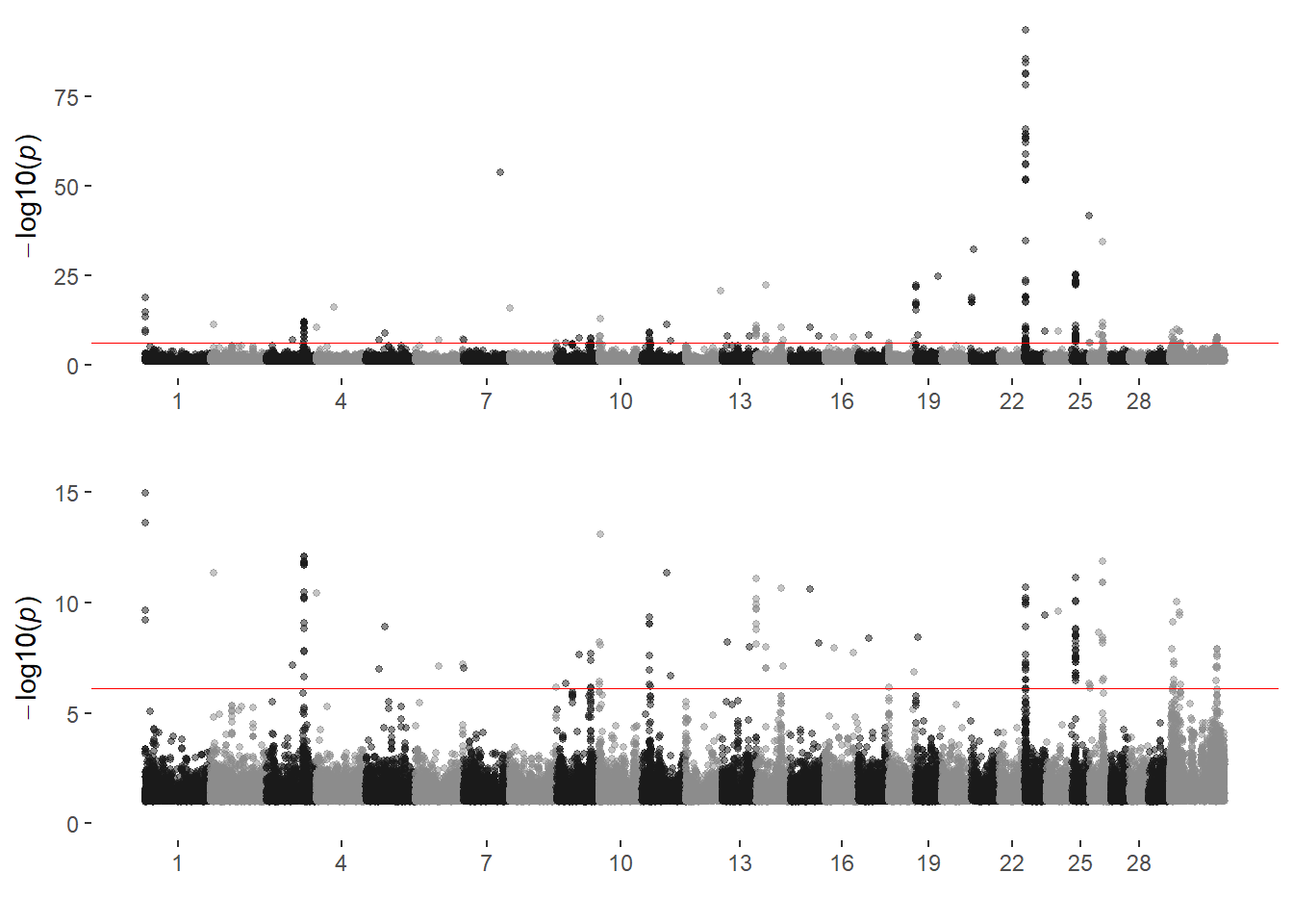
#Saving significant SNPs for highlighting in other plots:
raw_age_sigsnps =
  ran_gpsm_age %>%
    filter(p < 7.546167e-07) %>% .$SNP
Square Root
Square root transformed age as phenotype (Significance threshold - Bonferroni)
Green points indicate novel SNPs in this transformed analysis (at Bonferroni significance levels) that weren’t identified in the GPSM analysis of raw age.
plot_grid(
  ggmanhattan2(ran_gpsm_sqrtage,
               prune = 0.1,
               sig_threshold_p = 7.546167e-07,
               sigsnps = filter(ran_gpsm_sqrtage,
                                p < 7.546e-7 & !SNP %in% raw_age_sigsnps) %>%
                 .$SNP),
  ggmanhattan2(ran_gpsm_sqrtage,
               prune = 0.1,
               sig_threshold_p = 7.546167e-07,
               sigsnps = filter(ran_gpsm_sqrtage,
                                p < 7.546e-7 & !SNP %in% raw_age_sigsnps) %>%
                 .$SNP)+
    ylim(c(0,15)),
  nrow = 2)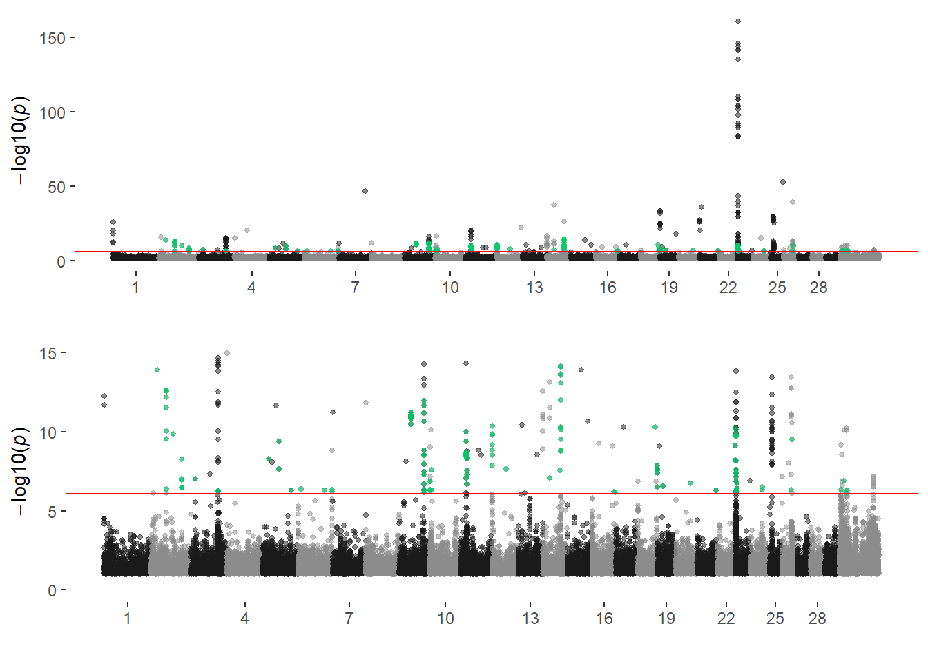
Cube Root
Cube Root Transformed Age Manahattan Plots (Significance threshold - Bonferroni)
Green points indicate novel SNPs in this transformed analysis (at Bonferroni significance levels) that weren’t identified in the GPSM analysis of raw age.
plot_grid(
  ggmanhattan2(ran_gpsm_cbrtage,
               prune = 0.1,
               sig_threshold_p = 7.546167e-07,
               sigsnps = filter(ran_gpsm_cbrtage,
                                p < 7.546e-7 & !SNP %in% raw_age_sigsnps) %>%
                 .$SNP),
  ggmanhattan2(ran_gpsm_cbrtage,
               prune = 0.1,
               sig_threshold_p = 7.546167e-07,
               sigsnps = filter(ran_gpsm_cbrtage,
                                p < 7.546e-7 & !SNP %in% raw_age_sigsnps) %>%
                 .$SNP)+
    ylim(c(0,15)),
  nrow = 2)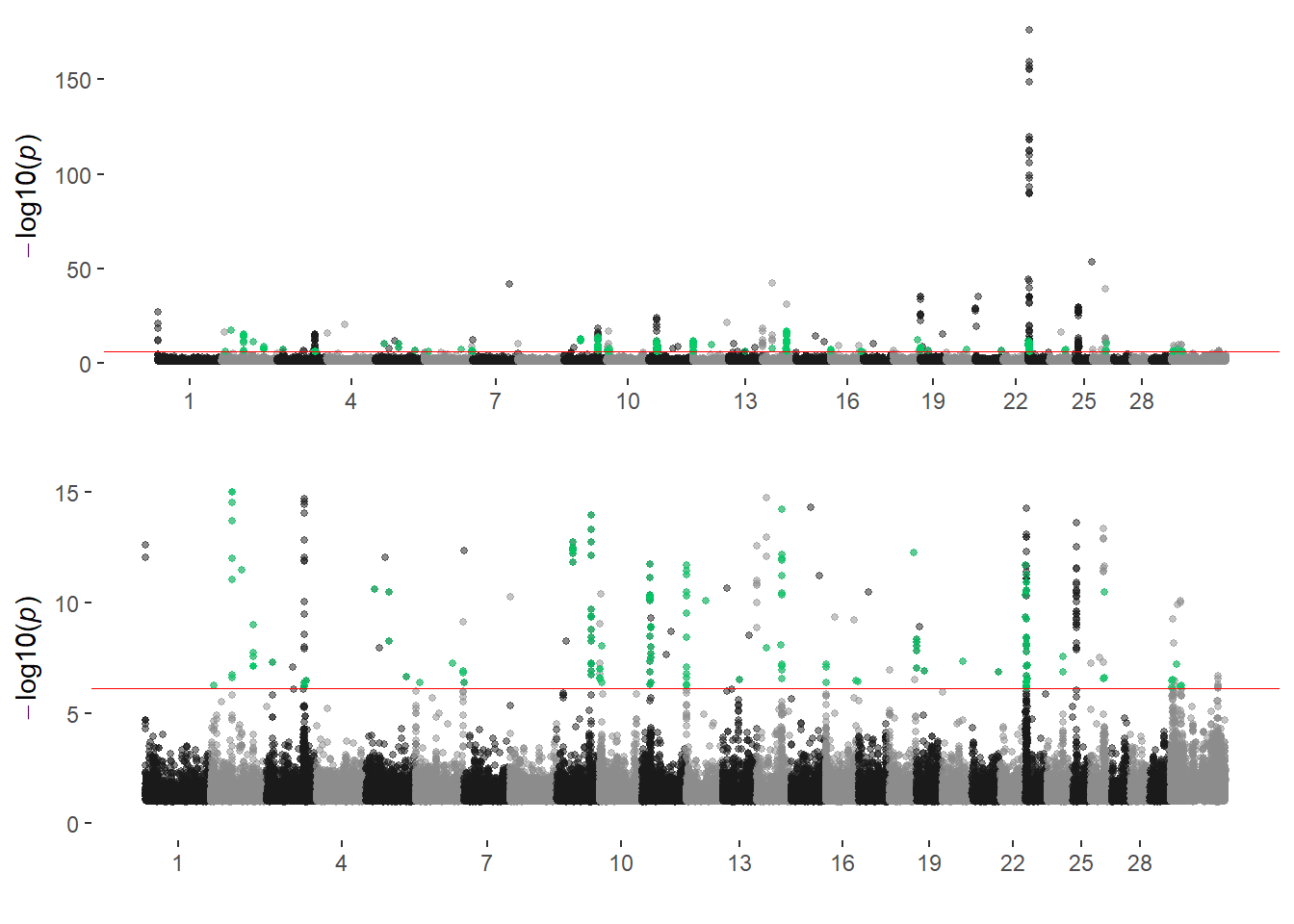
Box-Cox
Box-Cox Transformed Age Manahattan Plots (Significance threshold - Bonferroni)
Green points indicate novel SNPs in this transformed analysis (at Bonferroni significance levels) that weren’t identified in the GPSM analysis of raw age.
plot_grid(
  ggmanhattan2(ran_gpsm_bcage,
               prune = 0.1,
               sig_threshold_p = 7.546167e-07,
               sigsnps = filter(ran_gpsm_bcage,
                                p < 7.546e-7 & !SNP %in% raw_age_sigsnps) %>%
                 .$SNP),
  ggmanhattan2(ran_gpsm_bcage,
               prune = 0.1,
               sig_threshold_p = 7.546167e-07,
               sigsnps = filter(ran_gpsm_bcage,
                                p < 7.546e-7 & !SNP %in% raw_age_sigsnps) %>%
                 .$SNP)+
    ylim(c(0,15)),
  nrow = 2)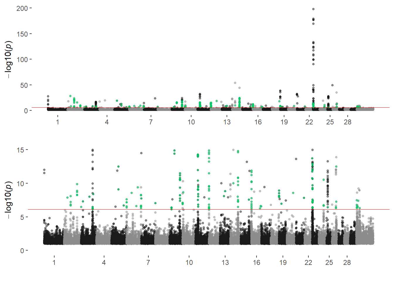
Log
Log Transformed Age Manahattan Plots (Significance threshold - Bonferroni)
Green points indicate novel SNPs in this transformed analysis (at Bonferroni significance levels) that weren’t identified in the GPSM analysis of raw age.
plot_grid(
  ggmanhattan2(ran_gpsm_logage,
               prune = 0.1,
               sig_threshold_p = 7.546167e-07,
               sigsnps = filter(ran_gpsm_logage,
                                p < 7.546e-7 & !SNP %in% raw_age_sigsnps) %>%
                 .$SNP),
  ggmanhattan2(ran_gpsm_logage,
               prune = 0.1,
               sig_threshold_p = 7.546167e-07,
               sigsnps = filter(ran_gpsm_logage,
                                p < 7.546e-7 & !SNP %in% raw_age_sigsnps) %>%
                 .$SNP)+
    ylim(c(0,15)),
  nrow = 2)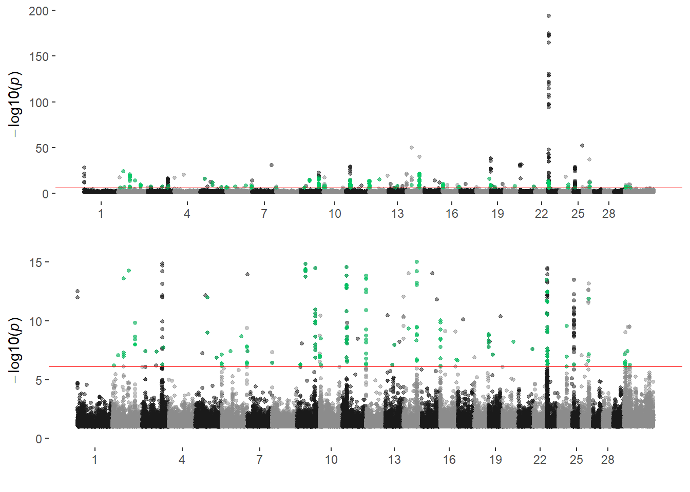
sessionInfo()R version 4.0.2 (2020-06-22)
Platform: x86_64-w64-mingw32/x64 (64-bit)
Running under: Windows 10 x64 (build 19041)
Matrix products: default
locale:
[1] LC_COLLATE=English_United States.1252
[2] LC_CTYPE=English_United States.1252
[3] LC_MONETARY=English_United States.1252
[4] LC_NUMERIC=C
[5] LC_TIME=English_United States.1252
attached base packages:
[1] stats graphics grDevices utils datasets methods base
other attached packages:
[1] viridis_0.5.1 viridisLite_0.3.0 cowplot_1.1.0 GALLO_0.99.0
[5] qvalue_2.20.0 pedigree_1.4 reshape_0.8.8 HaploSim_1.8.4
[9] Matrix_1.2-18 lubridate_1.7.9 forcats_0.5.0 stringr_1.4.0
[13] dplyr_1.0.2 readr_1.3.1 tidyr_1.1.2 tibble_3.0.3
[17] tidyverse_1.3.0 here_0.1 ggcorrplot_0.1.3 corrr_0.4.2
[21] factoextra_1.0.7 ggplot2_3.3.2 purrr_0.3.4 ggthemes_4.2.0
[25] maps_3.3.0 knitr_1.30 workflowr_1.6.2
loaded via a namespace (and not attached):
[1] fs_1.5.0 doParallel_1.0.15 RColorBrewer_1.1-2
[4] httr_1.4.2 rprojroot_1.3-2 dynamicTreeCut_1.63-1
[7] tools_4.0.2 backports_1.1.10 R6_2.4.1
[10] DBI_1.1.0 colorspace_1.4-1 withr_2.3.0
[13] gridExtra_2.3 tidyselect_1.1.0 compiler_4.0.2
[16] git2r_0.27.1 cli_2.0.2 rvest_0.3.6
[19] xml2_1.3.2 labeling_0.3 scales_1.1.1
[22] digest_0.6.25 rmarkdown_2.3 pkgconfig_2.0.3
[25] htmltools_0.5.0 dbplyr_1.4.4 rlang_0.4.7
[28] GlobalOptions_0.1.2 readxl_1.3.1 rstudioapi_0.11
[31] farver_2.0.3 shape_1.4.5 generics_0.0.2
[34] jsonlite_1.7.1 magrittr_1.5 Rcpp_1.0.5
[37] munsell_0.5.0 fansi_0.4.1 lifecycle_0.2.0
[40] stringi_1.5.3 whisker_0.4 yaml_2.2.1
[43] plyr_1.8.6 grid_4.0.2 blob_1.2.1
[46] parallel_4.0.2 promises_1.1.1 ggrepel_0.8.2
[49] crayon_1.3.4 lattice_0.20-41 haven_2.3.1
[52] splines_4.0.2 circlize_0.4.10 hms_0.5.3
[55] pillar_1.4.6 reshape2_1.4.4 codetools_0.2-16
[58] reprex_0.3.0 glue_1.4.2 evaluate_0.14
[61] unbalhaar_2.0 data.table_1.13.0 modelr_0.1.8
[64] vctrs_0.3.4 httpuv_1.5.4 foreach_1.5.0
[67] cellranger_1.1.0 gtable_0.3.0 assertthat_0.2.1
[70] xfun_0.17 broom_0.7.0 later_1.1.0.1
[73] iterators_1.0.12 ellipsis_0.3.1