Differential Gene Expression (DGE) Analysis
Last updated: 2024-04-11
Checks: 7 0
Knit directory: mecfs-dge-analysis/
This reproducible R Markdown analysis was created with workflowr (version 1.7.1). The Checks tab describes the reproducibility checks that were applied when the results were created. The Past versions tab lists the development history.
Great! Since the R Markdown file has been committed to the Git repository, you know the exact version of the code that produced these results.
Great job! The global environment was empty. Objects defined in the global environment can affect the analysis in your R Markdown file in unknown ways. For reproduciblity it’s best to always run the code in an empty environment.
The command set.seed(20230618) was run prior to running
the code in the R Markdown file. Setting a seed ensures that any results
that rely on randomness, e.g. subsampling or permutations, are
reproducible.
Great job! Recording the operating system, R version, and package versions is critical for reproducibility.
Nice! There were no cached chunks for this analysis, so you can be confident that you successfully produced the results during this run.
Great job! Using relative paths to the files within your workflowr project makes it easier to run your code on other machines.
Great! You are using Git for version control. Tracking code development and connecting the code version to the results is critical for reproducibility.
The results in this page were generated with repository version f24bf2c. See the Past versions tab to see a history of the changes made to the R Markdown and HTML files.
Note that you need to be careful to ensure that all relevant files for
the analysis have been committed to Git prior to generating the results
(you can use wflow_publish or
wflow_git_commit). workflowr only checks the R Markdown
file, but you know if there are other scripts or data files that it
depends on. Below is the status of the Git repository when the results
were generated:
Ignored files:
    Ignored:    .DS_Store
    Ignored:    .Rhistory
    Ignored:    .Rproj.user/
    Ignored:    analysis/.DS_Store
    Ignored:    data/.DS_Store
    Ignored:    omnipathr-log/
    Ignored:    output/.DS_Store
    Ignored:    output/batch-correction-limma/
    Ignored:    output/condition-analysis.RData
    Ignored:    output/subsetted-condition-analysis.RData

Untracked files:
    Untracked:  output/counts_vst_limma_subsetted.csv
    Untracked:  output/counts_vst_subsetted..csv
    Untracked:  output/res_aff_vs_unaff_df_sub_genename.csv
    Untracked:  output/res_aff_vs_unaff_df_sub_genename_05.csv
    Untracked:  output/res_aff_vs_unaff_df_sub_genename_padj1.csv
    Untracked:  output/res_aff_vs_unaff_significant_subsetted_mygene.csv
    Untracked:  output/res_aff_vs_unaff_significant_subsetted_samples.csv
    Untracked:  output/res_aff_vs_unaff_sub.csv

Unstaged changes:
    Modified:   output/bysample_upset.png
    Modified:   output/counts_vst.csv
    Modified:   output/counts_vst_female.csv
    Modified:   output/counts_vst_limma.csv
    Modified:   output/counts_vst_limma_female.csv
Note that any generated files, e.g. HTML, png, CSS, etc., are not included in this status report because it is ok for generated content to have uncommitted changes.
These are the previous versions of the repository in which changes were
made to the R Markdown
(analysis/subsetted-condition-analysis.Rmd) and HTML
(docs/subsetted-condition-analysis.html) files. If you’ve
configured a remote Git repository (see ?wflow_git_remote),
click on the hyperlinks in the table below to view the files as they
were in that past version.
| File | Version | Author | Date | Message |
|---|---|---|---|---|
| Rmd | f24bf2c | sdhutchins | 2024-04-11 | workflowr::wflow_publish(files = "analysis/subsetted-condition-analysis.Rmd") |
| html | 1e45c53 | sdhutchins | 2024-04-09 | Build site. |
| Rmd | 684c0de | sdhutchins | 2024-04-09 | Add subsetted analysis. |
| html | 1804028 | sdhutchins | 2024-04-08 | Update metadata. |
| Rmd | 4d5d173 | sdhutchins | 2024-04-08 | Create subsetted analysis. |
| html | 0c1afe6 | sdhutchins | 2024-03-13 | Build site. |
| Rmd | 1fa52ee | sdhutchins | 2024-03-13 | workflowr::wflow_publish(files = "analysis/subsetted-condition-analysis.Rmd") |
DGE Analysis Setup
Ensure you have all necessary libraries installed and load the helper code.
At a later date, renv will be integrated to ensure
reproducibility of this analysis.
Use the below code to install these packages:
# Install packages from CRAN
install.packages(c("tidyverse", "RColorBrewer", "pheatmap", "gprofiler2", "plotly", "ggupset"))

# Install packages from Bioconductor
install.packages("BiocManager")
BiocManager::install(c("DESeq2", "genefilter", "limma", "biomaRt", "mygene"))
library(tidyverse) # Available via CRAN
library(DESeq2) # Available via Bioconductor
library(RColorBrewer) # Available via CRAN
library(pheatmap) # Available via CRAN
library(genefilter) # Available via Bioconductor
library(limma) # Available via Bioconductor
library(gprofiler2) # Available via CRAN
library(biomaRt) # Available via Bioconductor
library(plotly) # Available via CRAN
library(ggpubr)
library(rmarkdown)
library(ggupset)
library(clusterProfiler)
library(DOSE)
library(org.Hs.eg.db) # Available via Bioconductor
library(UpSetR)
library(ggrepel)
library(ReactomePA)Data Import
We will be importing counts data from the star-salmon pipeline and our metadata for the project which is hosted on Box. This also ensures data is properly ordered by sample id.
counts <- read_tsv("data/star-salmon/salmon.merged.gene_counts_length_scaled.tsv")

# Import variants of interest
genes_of_interest <- read_csv("data/Patient_Genes_2024_03_05.csv")
genes_of_interest <- unique(genes_of_interest$Genes)
genes_of_interest <- genes_of_interest[!is.na(genes_of_interest)]

# Use first column (gene_id) for row names
counts <- data.frame(counts, row.names = 1)
counts$Ensembl_ID <- row.names(counts)
drop <- c("Ensembl_ID", "gene_name")
gene_info <- counts[, drop]
counts <- counts[, !(names(counts) %in% drop)] # remove both columns

# Import metadata
sample_metadata <- read_csv("data/MECFS_RNAseq_metadata_2024_03_14.csv")
row.names(sample_metadata) <- sample_metadata$ID

# Assuming counts is your counts dataframe and sample_metadata is your metadata dataframe
# Call the function with the appropriate column names
counts <- rename_counts_columns(counts, sample_metadata, "ID", "RNA_Samples_id")

# Check that data is ordered properly
sample_metadata <- check_order(sample_metadata = sample_metadata, counts = counts)

genes_biomart <- retrieve_gene_info(values = gene_info$Ensembl_ID, filters = "ensembl_gene_id_version")
DESeq2 Analysis
sample_metadata$Family <- factor(sample_metadata$Family)
sample_metadata$Affected <- factor(sample_metadata$Affected)
sample_metadata$Batch <- factor(sample_metadata$Batch)
sample_metadata$Sex <- factor(sample_metadata$Sex)
sample_metadata$Ancestry <- factor(sample_metadata$Ancestry)
sample_metadata$SubCategory <- factor(sample_metadata$SubCategory)
sample_metadata$CombinedCategory <- factor(sample_metadata$CombinedCategory)

# Account for Family later but batch is accounted for
# Accounting for another factor seems to be an issue.
dds <- DESeqDataSetFromMatrix(
  countData = round(counts), colData = sample_metadata,
  design = ~ Batch + Affected
)

# Pre-filtering: Keep only rows that have at least 10 reads total
keep <- rowSums(counts(dds)) >= 10
dds <- dds[keep, ]

# Remove samples from family's with multiple samples
remove_multiple_fam <- c("8", "12", "19", "21", "23", "27")

# Save excluded/removed samples
# Code is commented out since this is for 1 time usage
# excluded_samples_df <- filter(sample_metadata,
#                        ID %in% remove_multiple_fam)
# write.csv(excluded_samples_df, "data/excluded_samples_df.csv")

# Create a logical vector to index the columns you want to keep
kept_fam_members <- !(colnames(dds) %in% remove_multiple_fam)
dds <- dds[, kept_fam_members]

# Run DESeq function
dds <- DESeq(dds)

# Normalize gene counts for differences in seq. depth/global differences
counts_norm <- counts(dds, normalized = TRUE)
Data transformation and visualization
Perform count data transformation by variance stabilizing transformation (vst) on normalized counts.
vsd <- vst(dds, blind = FALSE)Batch correction with limma
counts_vst <- assay(vsd)
write.csv(counts_vst, file = "output/counts_vst_subsetted..csv")
mm <- model.matrix(~ Batch + Affected, colData(vsd))

counts_vst_limma <- limma::removeBatchEffect(counts_vst, batch = vsd$Batch, design = mm)
Coefficients not estimable: batch1 batch2 write.csv(counts_vst_limma, file = "output/counts_vst_limma_subsetted.csv")
vsd_limma <- vsd
assay(vsd_limma) <- counts_vst_limmaSample distances heatmap
sample_dists_all <- dist(t(assay(vsd_limma)))
sample_dist_matrix_all <- as.matrix(sample_dists_all)
rownames(sample_dist_matrix_all) <- paste(vsd_limma$Batch, vsd_limma$Affected, sep = " | ")
colnames(sample_dist_matrix_all) <- paste(vsd_limma$ID, vsd_limma$Affected, sep = " | ")
colors <- colorRampPalette(rev(brewer.pal(9, "Blues")))(255)

pheatmap(sample_dist_matrix_all, clustering_distance_rows = sample_dists_all, clustering_distance_cols = sample_dists_all, col = colors)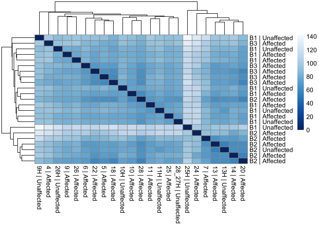
Principal Components Analysis
Our below PCA shows that there does not seem to be a batch-related effect occurring after using limma. However, we can see that our 3 male samples are grouping. Given this knowledge, removing them from downstream analyses is the best option.
pca_data_all <- plotPCA(vsd_limma, intgroup = c("Batch", "Affected", "Sex"), returnData = TRUE)
percent_var_all <- round(100 * attr(pca_data_all, "percentVar"))

ggplot(pca_data_all, aes(PC1, PC2)) +
  geom_point(aes(colour = Affected, fill = Sex, shape = Batch), size = 4) +
  scale_shape_manual(values = c(21, 22, 23)) +
  scale_fill_manual(values = c("white", "gray")) +
  scale_color_manual(values = c("blue", "red")) +
  geom_text(aes(label = name),
    data = subset(pca_data_all, PC2 < -18 | PC1 < -30),
    vjust = -1, hjust = 0.5, size = 2.5
  ) +
  xlab(paste0("PC1: ", percent_var_all[1], "% variance")) +
  ylab(paste0("PC2: ", percent_var_all[2], "% variance")) +
  coord_fixed()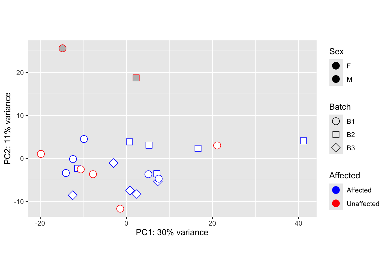
pca_data_all <- plotPCA(vsd_limma, intgroup = c("Affected", "Sex", "CombinedCategory"), returnData = TRUE)
percent_var_all <- round(100 * attr(pca_data_all, "percentVar"))

ggplot(pca_data_all, aes(PC1, PC2)) +
  geom_point(aes(colour = CombinedCategory, fill = Sex, shape = Affected), size = 4) +
  scale_shape_manual(values = c(21, 22, 23)) +
  scale_fill_manual(values = c("white", "gray")) +
  geom_text(aes(label = name), vjust = -1, hjust = 0.65, size = 5) +
  # geom_text_repel(aes(label = name), size = 5, vjust = -1, hjust = -0.65) +
  xlab(paste0("PC1: ", percent_var_all[1], "% variance")) +
  ylab(paste0("PC2: ", percent_var_all[2], "% variance")) +
  coord_fixed()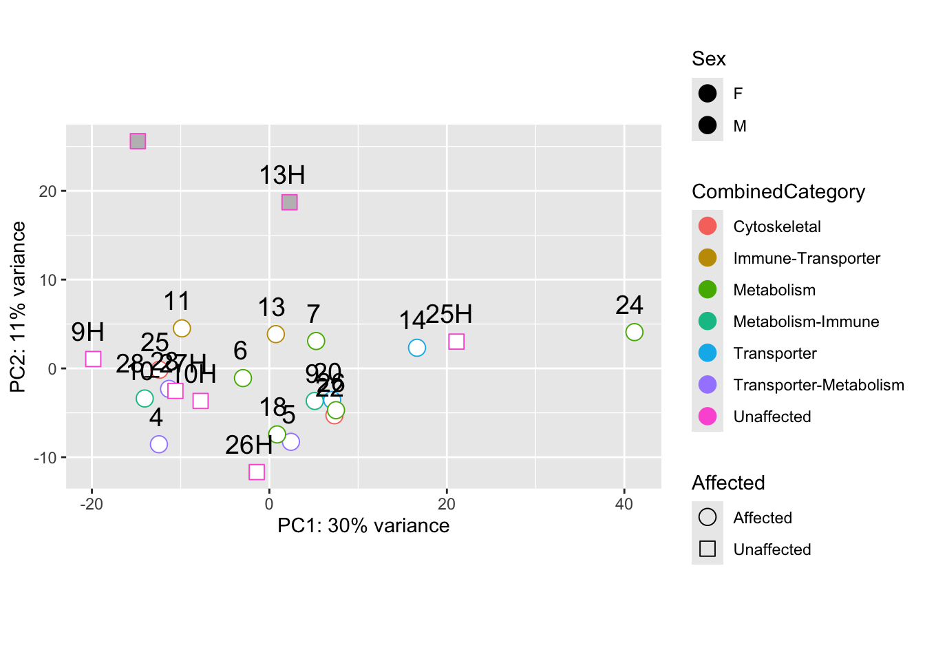
pca_data <- plotPCA(vsd_limma, intgroup = c("Sex", "Affected"), returnData = TRUE)
percent_var <- round(100 * attr(pca_data, "percentVar"))

ggplot(pca_data, aes(PC1, PC2)) +
  geom_point(aes(shape = Sex, colour = Affected), size = 5) +
  scale_color_manual(
    values = c("blue", "red"),
    name = "Affected Status",
    labels = c("Unaffected", "Affected")
  ) +
  scale_shape_manual(
    name = "Sex",
    labels = c("Male", "Female"),
    values = c(16, 17)
  ) + # Example shapes, change as needed
  geom_text_repel(aes(label = name), size = 5, vjust = -2, hjust = -0.65) +
  xlab(paste0("PC1: ", percent_var[1], "% variance")) +
  ylab(paste0("PC2: ", percent_var[2], "% variance")) +
  coord_fixed()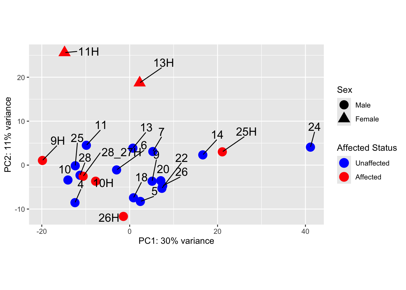
pca_data_all <- plotPCA(vsd_limma, intgroup = c("CombinedCategory"), returnData = TRUE)
percent_var_all <- round(100 * attr(pca_data_all, "percentVar"))

ggplot(pca_data_all, aes(PC1, PC2)) +
  geom_point(aes(colour = CombinedCategory), size = 5) +
  scale_colour_manual(
    values = c(
      "#B3DE69", "#FFFFB3", "#BEBADA", "#FB8072", "#80B1D3",
      "#FCCDE5", "#8DD3C7", "#000000"
    ),
    name = "Category"
  ) +
  # geom_text(aes(label = name), vjust = -.75, hjust = -.5, size = 3) +
  # geom_text_repel(aes(label = name), size = 5, vjust = -2, hjust = -0.65) +
  geom_text_repel(aes(label = name), size = 3) +
  xlab(paste0("PC1: ", percent_var_all[1], "% variance")) +
  ylab(paste0("PC2: ", percent_var_all[2], "% variance")) +
  ggthemes::theme_clean()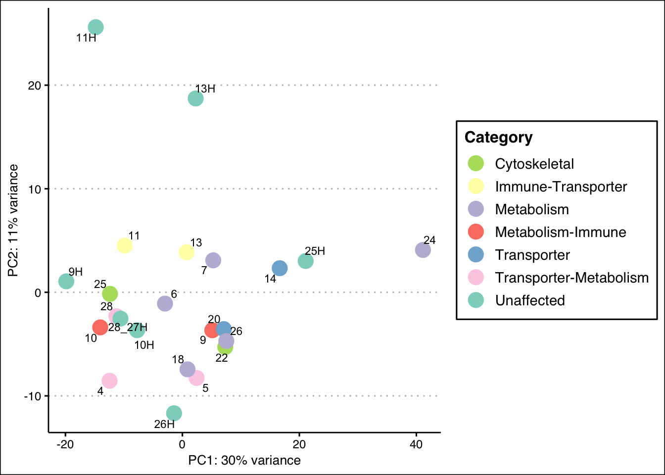
Heatmap of all genes, top 50 & top 100 genes
# Specify annotation colors by columns
# Use RColorBrewer::brewer.pal(n=10, name="Set1")
category_colors <- c(
  "Autoimmune disorder" = "#B3DE69",
  "Immunodeficiency" = "#FFFFB3",
  "Channelopathy" = "#BEBADA",
  "Inflammatory disorder" = "#FB8072",
  "Metabolic disorder" = "#80B1D3",
  "Mitochondrial disorder" = "#FCCDE5",
  "Neurologic disorder" = "#D9D9D9",
  "Myasthenic disorder" = "#FDB462",
  "Neuropathy" = "#8DD3C7",
  "Unaffected" = "#001111"
)

combined_category_colors <- c(
  "Transporter-Metabolism" = "#E41A1C", # Dark green
  "Metabolism" = "#377EB8", # Dark orange
  "Metabolism-Immune" = "#4DAF4A", # Light purple
  "Immune-Transporter" = "#984EA3", # Magenta
  "Transporter" = "#FF7F00", # Light green
  "Cytoskeletal" = "#FFFF33", # Mustard yellow
  "Transporter-Immune-Metabolism" = "#F781BF", # Brown
  "Unaffected" = "#000000" # Dark grey
)


# Specify colors
ann_colors <- list(
  Batch = c(B1 = "purple", B2 = "firebrick", B3 = "yellow"),
  Affected = c(Affected = "green", Unaffected = "navy"),
  SubCategory = category_colors,
  CombinedCategory = combined_category_colors
)

ann_colors2 <- list(
  Batch = c(B1 = "purple", B2 = "firebrick", B3 = "yellow"),
  Affected = c(Affected = "green", Unaffected = "navy"),
  SubCategory = category_colors,
  CombinedCategory = combined_category_colors
)
This is a heatmap of the top 50 genes with the highest variance across samples
top_var_genes <- head(order(-rowVars(assay(vsd_limma))), 50)
mat <- assay(vsd_limma)[top_var_genes, ]
mat <- mat - rowMeans(mat)
df <- as.data.frame(colData(vsd_limma)[, c("Batch", "Affected", "CombinedCategory")])

ensembl_to_gene <- setNames(gene_info$gene_name, gene_info$Ensembl_ID)

# Get the current row names of the matrix 'mat'
current_ensembl_ids <- rownames(mat)

# Find the corresponding gene names for the Ensembl IDs
new_row_names <- ensembl_to_gene[current_ensembl_ids]

# Set the new row names for the matrix 'mat'
rownames(mat) <- new_row_names

ComplexHeatmap::pheatmap(mat, annotation_col = df, annotation_colors = ann_colors2,
                         fontsize = 5, angle_col = c("0"))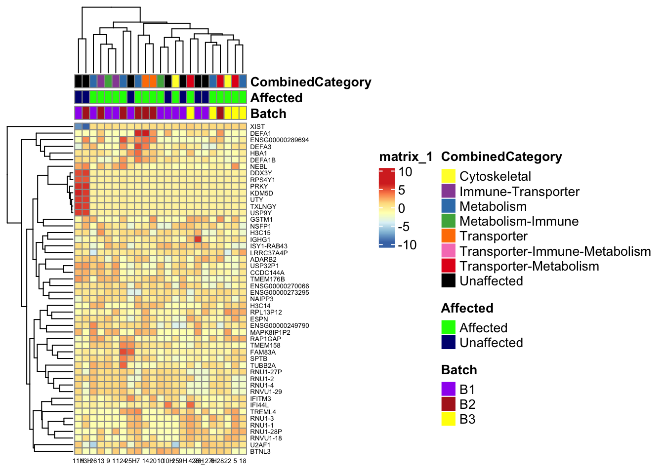
This is a heatmap of the top 50 genes with the highest variance across all samples.
top_var_genes_all <- head(order(-rowVars(assay(vsd_limma))), 50)
mat_all <- assay(vsd_limma)[top_var_genes_all, ]
mat_all <- mat_all - rowMeans(mat_all)
df_all <- as.data.frame(colData(vsd_limma)[, c("Batch", "Affected", "SubCategory")])
df_affcat <- as.data.frame(colData(vsd_limma)[, c("Affected", "CombinedCategory")])

ensembl_to_gene <- setNames(gene_info$gene_name, gene_info$Ensembl_ID)

# Get the current row names of the matrix 'mat'
current_ensembl_ids_all <- rownames(mat_all)

# Find the corresponding gene names for the Ensembl IDs
new_row_names_all <- ensembl_to_gene[current_ensembl_ids_all]

# Set the new row names for the matrix 'mat'
rownames(mat_all) <- new_row_names_all

pheatmap(mat_all, annotation_col = df_all, annotation_colors = ann_colors, fontsize = 5)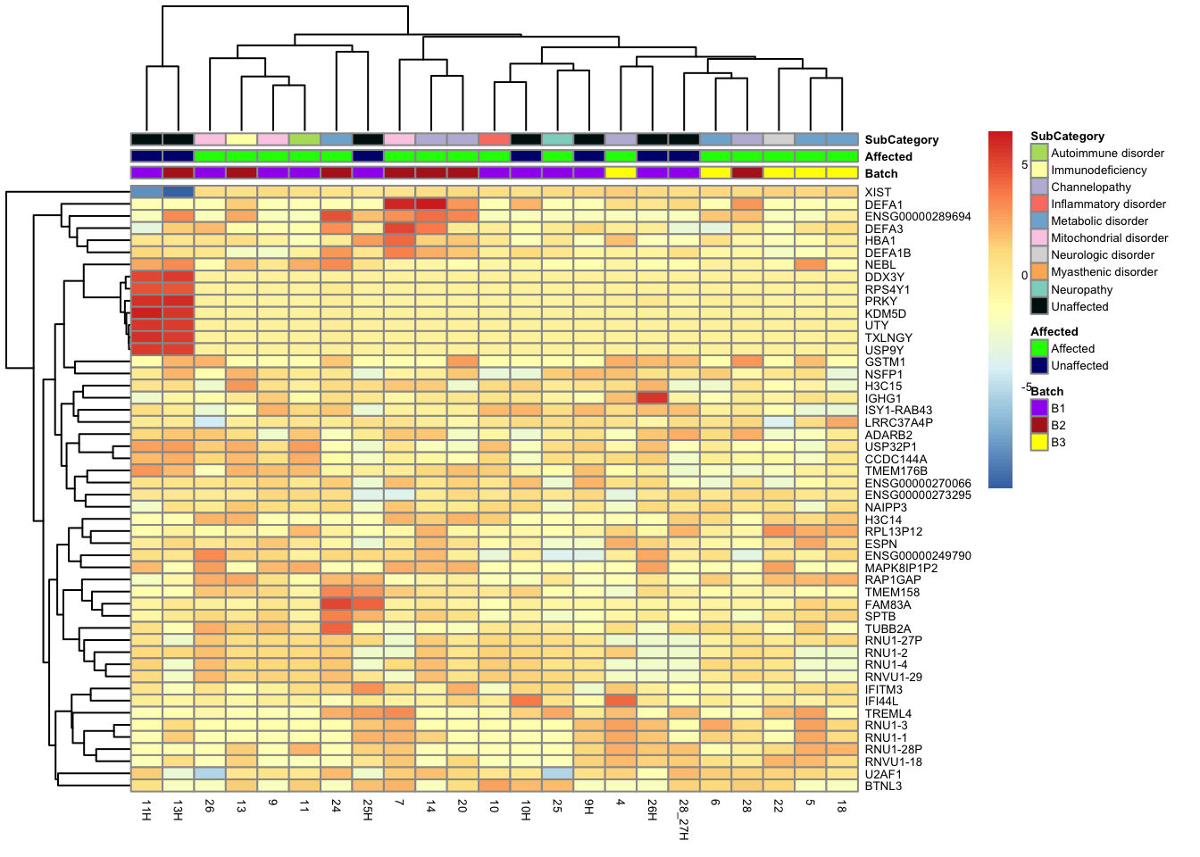
pheatmap(mat_all, annotation_col = df_affcat, annotation_colors = ann_colors2, fontsize = 5)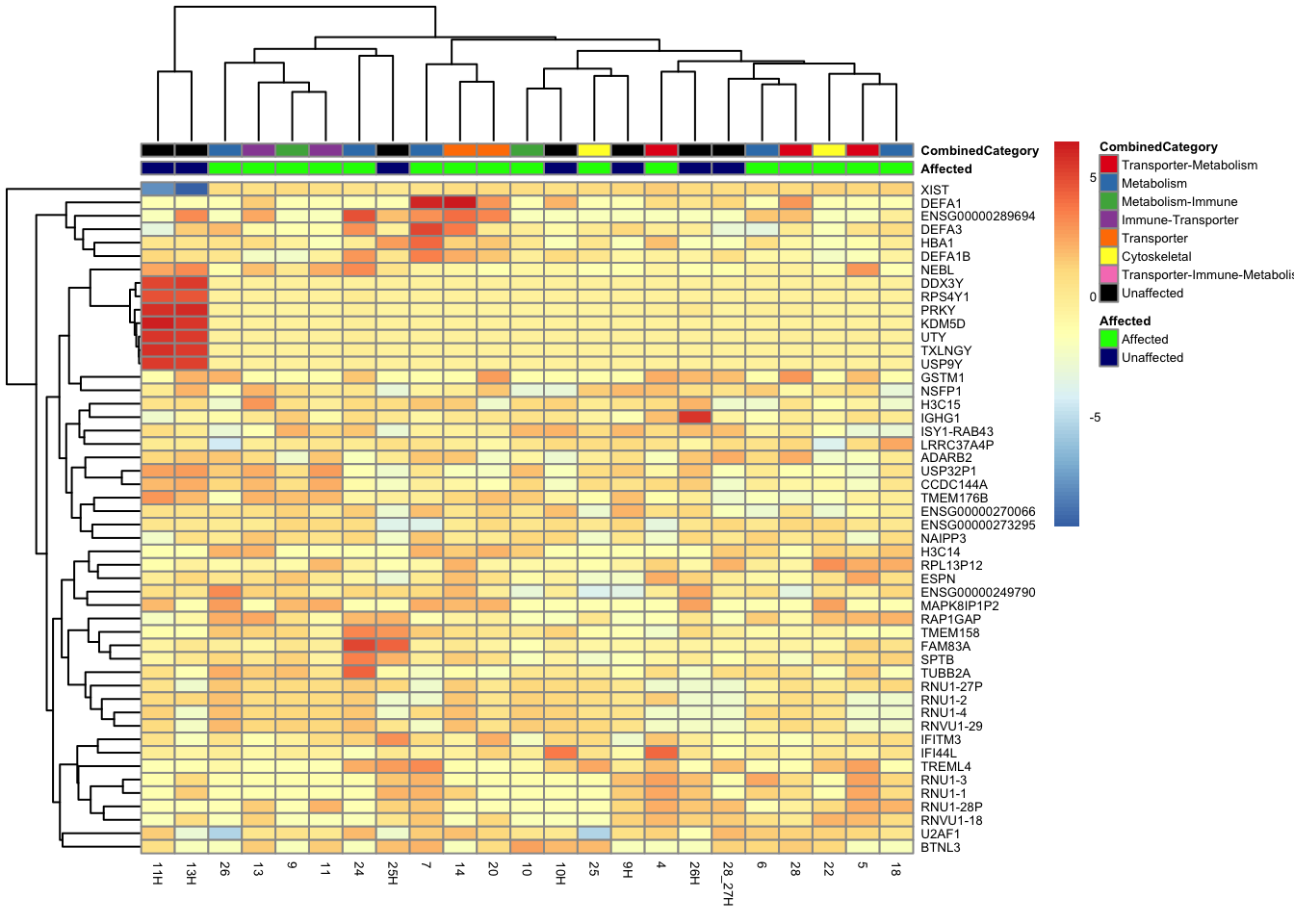
This is a heatmap of the top 100 genes with the highest variance across
top_var_genes_100_all <- head(order(-rowVars(assay(vsd_limma))), 100)
mat_100_all <- assay(vsd_limma)[top_var_genes_100_all, ]
mat_100_all <- mat_100_all - rowMeans(mat_100_all)
df_100_all <- as.data.frame(colData(vsd_limma)[, c("Affected", "SubCategory")])

ensembl_to_gene <- setNames(gene_info$gene_name, gene_info$Ensembl_ID)

# Get the current row names of the matrix 'mat'
current_ensembl_ids_100_all <- rownames(mat_100_all)

# Find the corresponding gene names for the Ensembl IDs
new_row_names_100_all <- ensembl_to_gene[current_ensembl_ids_100_all]

# Set the new row names for the matrix 'mat'
rownames(mat_100_all) <- new_row_names_100_all

pheatmap(mat_100_all, annotation_col = df_100_all, annotation_colors = ann_colors2, fontsize = 6)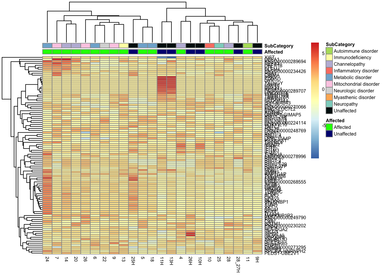
Comparison/Contrast of Affected_Affected_vs_Unaffected
res_aff_vs_unaff_sub <- results(dds, contrast = c("Affected", "Affected", "Unaffected"))
res_aff_vs_unaff_df_sub <- process_and_save_results(
  res_aff_vs_unaff_sub,
  "output/res_aff_vs_unaff_sub.csv"
)
res_aff_vs_unaff_df_sub <- arrange(res_aff_vs_unaff_df_sub, padj)
res_aff_vs_unaff_df_05_sub <- subset(res_aff_vs_unaff_df_sub, padj < 0.05)
res_aff_vs_unaff_df_1_sub <- subset(res_aff_vs_unaff_df_sub, padj < 0.05)

summary(res_aff_vs_unaff_sub)
out of 29623 with nonzero total read count
adjusted p-value < 0.1
LFC > 0 (up)       : 22, 0.074%
LFC < 0 (down)     : 33, 0.11%
outliers [1]       : 219, 0.74%
low counts [2]     : 0, 0%
(mean count < 0)
[1] see 'cooksCutoff' argument of ?results
[2] see 'independentFiltering' argument of ?results
topgenes_byensemblid_sub <- head(rownames(res_aff_vs_unaff_df_sub), 100)
topgenes_aff_vs_unaff_05_sub <- assay(vsd_limma)[topgenes_byensemblid_sub, ]
topgenes_aff_vs_unaff_05_sub <- topgenes_aff_vs_unaff_05_sub - rowMeans(topgenes_aff_vs_unaff_05_sub)
ensembl_to_gene_sub <- setNames(gene_info$gene_name, gene_info$Ensembl_ID)
# Get the current row names of the matrix 'mat'
current_ensembl_ids_sub <- rownames(topgenes_aff_vs_unaff_05_sub)
# Find the corresponding gene names for the Ensembl IDs
new_row_names_sub <- ensembl_to_gene_sub[current_ensembl_ids_sub]
# Set the new row names for the matrix 'mat'
rownames(topgenes_aff_vs_unaff_05_sub) <- new_row_names_sub
topgenes_aff_vs_unaff_05_sub <- topgenes_aff_vs_unaff_05_sub[order(row.names(topgenes_aff_vs_unaff_05_sub)), ]
df_sub <- as.data.frame(colData(vsd_limma)[, c("Affected", "CombinedCategory")])
pheatmap(topgenes_aff_vs_unaff_05_sub, annotation_col = df_sub, annotation_colors = ann_colors2, fontsize = 5, angle_col = c("0"))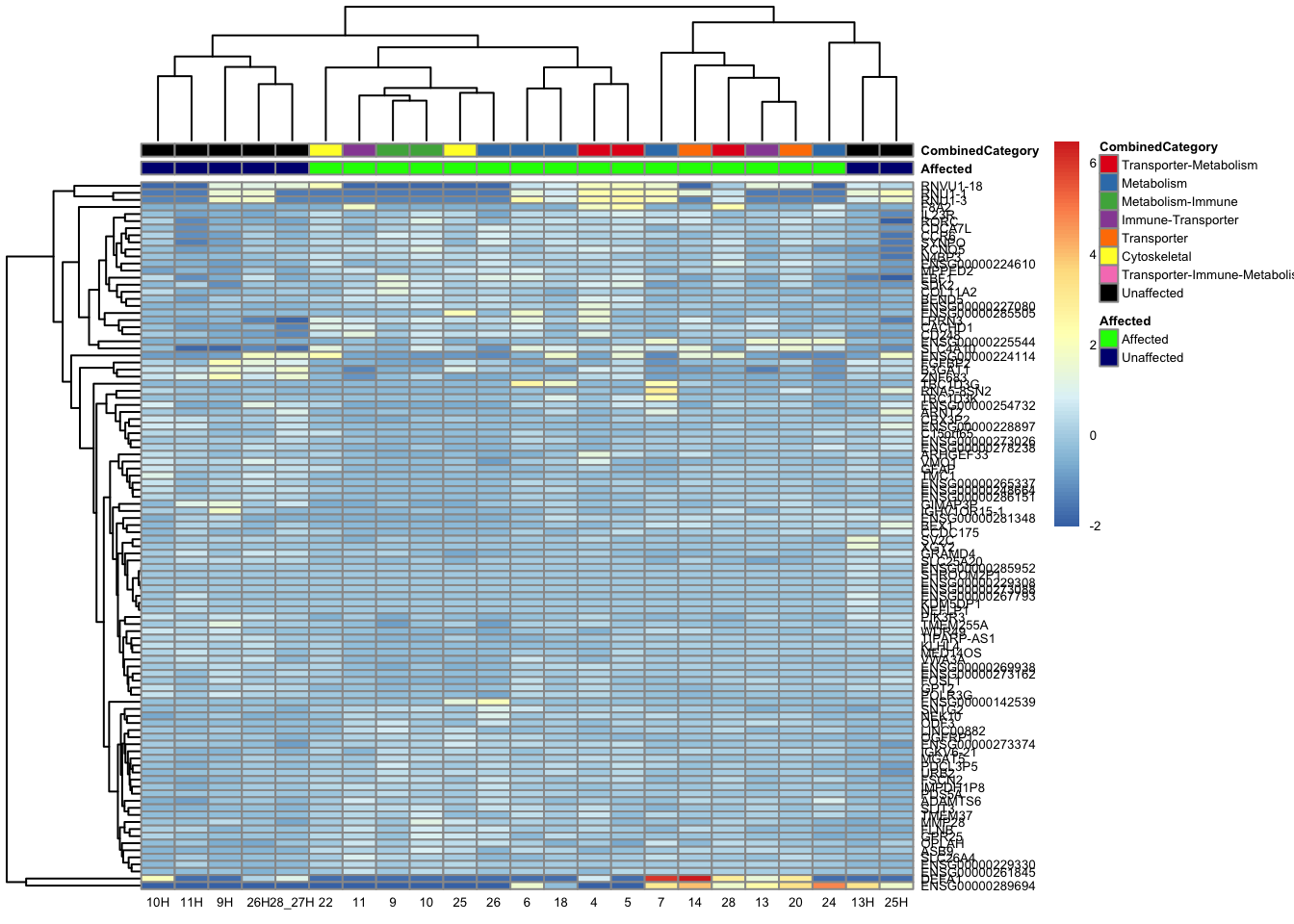
topgenes_byensemblid_sub <- head(rownames(res_aff_vs_unaff_df_sub), 100)
topgenes_aff_vs_unaff_05_sub <- assay(vsd_limma)[topgenes_byensemblid_sub, ]
topgenes_aff_vs_unaff_05_sub <- topgenes_aff_vs_unaff_05_sub - rowMeans(topgenes_aff_vs_unaff_05_sub)

ensembl_to_gene_sub <- setNames(gene_info$gene_name, gene_info$Ensembl_ID)

# Get the current row names of the matrix 'mat'
current_ensembl_ids_sub <- rownames(topgenes_aff_vs_unaff_05_sub)

# Find the corresponding gene names for the Ensembl IDs
new_row_names_sub <- ensembl_to_gene_sub[current_ensembl_ids_sub]

# Set the new row names for the matrix 'mat'
rownames(topgenes_aff_vs_unaff_05_sub) <- new_row_names_sub

topgenes_aff_vs_unaff_05_sub <- topgenes_aff_vs_unaff_05_sub[order(row.names(topgenes_aff_vs_unaff_05_sub)), ]

df_sub <- as.data.frame(colData(vsd_limma)[, c("Affected", "SubCategory", "CombinedCategory")])
pheatmap(topgenes_aff_vs_unaff_05_sub, annotation_col = df_sub, annotation_colors = ann_colors2, fontsize = 5, angle_col = 0)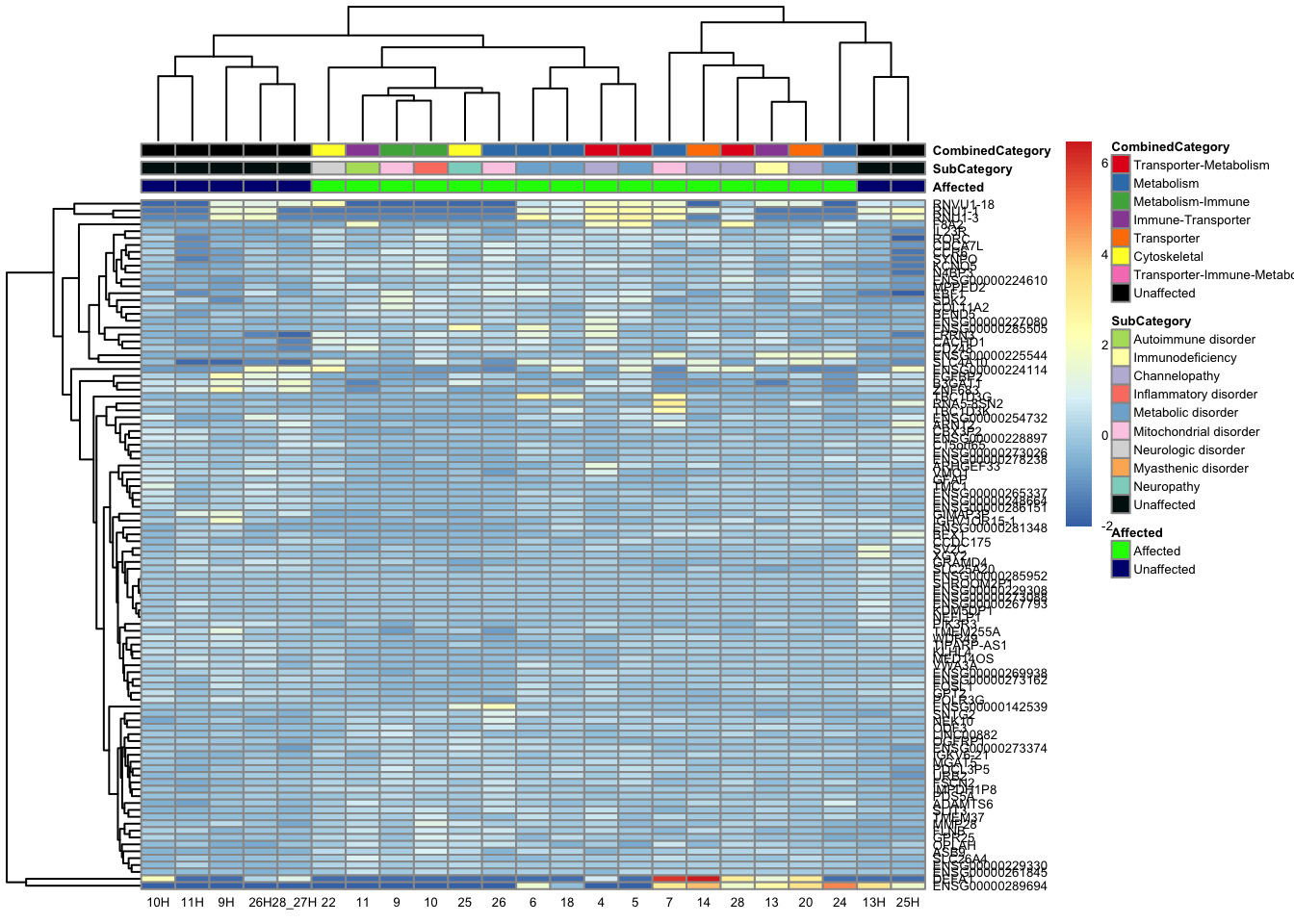
topgenes_byensemblid_sub <- head(rownames(res_aff_vs_unaff_df_sub), 50)
topgenes_aff_vs_unaff_05_sub <- assay(vsd_limma)[topgenes_byensemblid_sub, ]
topgenes_aff_vs_unaff_05_sub <- topgenes_aff_vs_unaff_05_sub - rowMeans(topgenes_aff_vs_unaff_05_sub)

ensembl_to_gene_sub <- setNames(gene_info$gene_name, gene_info$Ensembl_ID)

# Get the current row names of the matrix 'mat'
current_ensembl_ids_sub <- rownames(topgenes_aff_vs_unaff_05_sub)

# Find the corresponding gene names for the Ensembl IDs
new_row_names_sub <- ensembl_to_gene_sub[current_ensembl_ids_sub]

# Set the new row names for the matrix 'mat'
rownames(topgenes_aff_vs_unaff_05_sub) <- new_row_names_sub

topgenes_aff_vs_unaff_05_sub <- topgenes_aff_vs_unaff_05_sub[order(row.names(topgenes_aff_vs_unaff_05_sub)), ]

df_sub <- df <- colData(vsd_limma) %>%
  as.data.frame() %>%
  dplyr::select(CombinedCategory)
pheatmap(topgenes_aff_vs_unaff_05_sub, annotation_col = df_sub, annotation_colors = ann_colors2, fontsize = 5, angle_col = 0)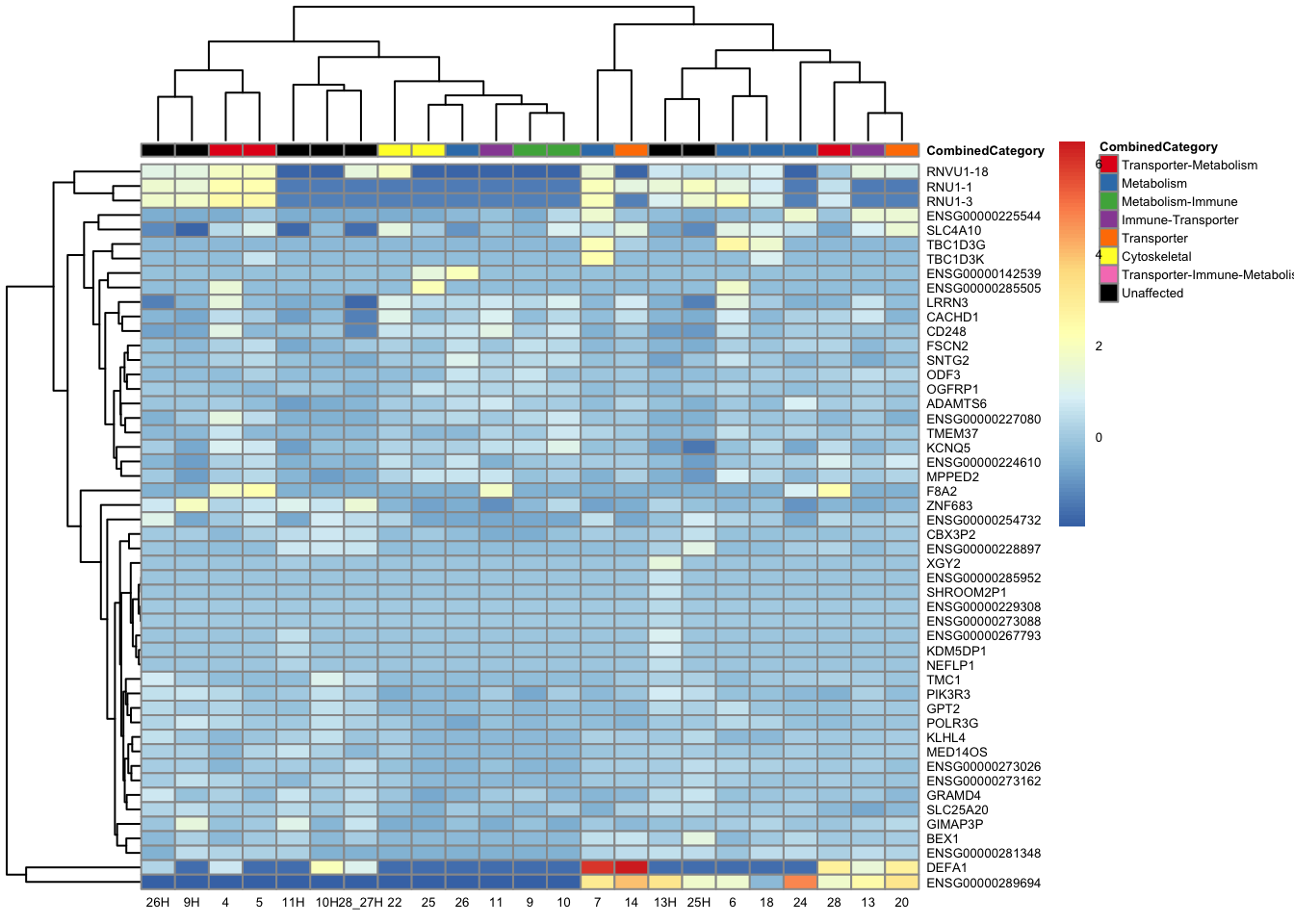
topgenes_byensemblid_sub <- head(rownames(res_aff_vs_unaff_df_sub), 50)
topgenes_aff_vs_unaff_05_sub <- assay(vsd_limma)[topgenes_byensemblid_sub, ]
topgenes_aff_vs_unaff_05_sub <- topgenes_aff_vs_unaff_05_sub - rowMeans(topgenes_aff_vs_unaff_05_sub)

ensembl_to_gene_sub <- setNames(gene_info$gene_name, gene_info$Ensembl_ID)

# Get the current row names of the matrix 'mat'
current_ensembl_ids_sub <- rownames(topgenes_aff_vs_unaff_05_sub)

# Find the corresponding gene names for the Ensembl IDs
new_row_names_sub <- ensembl_to_gene_sub[current_ensembl_ids_sub]

# Set the new row names for the matrix 'mat'
rownames(topgenes_aff_vs_unaff_05_sub) <- new_row_names_sub

topgenes_aff_vs_unaff_05_sub <- topgenes_aff_vs_unaff_05_sub[order(row.names(topgenes_aff_vs_unaff_05_sub)), ]

df_sub <- df <- colData(vsd_limma) %>%
  as.data.frame() %>%
  dplyr::select(Affected, SubCategory, CombinedCategory)
pheatmap(topgenes_aff_vs_unaff_05_sub, annotation_col = df_sub,
         annotation_colors = ann_colors2, fontsize = 5, angle_col = 0)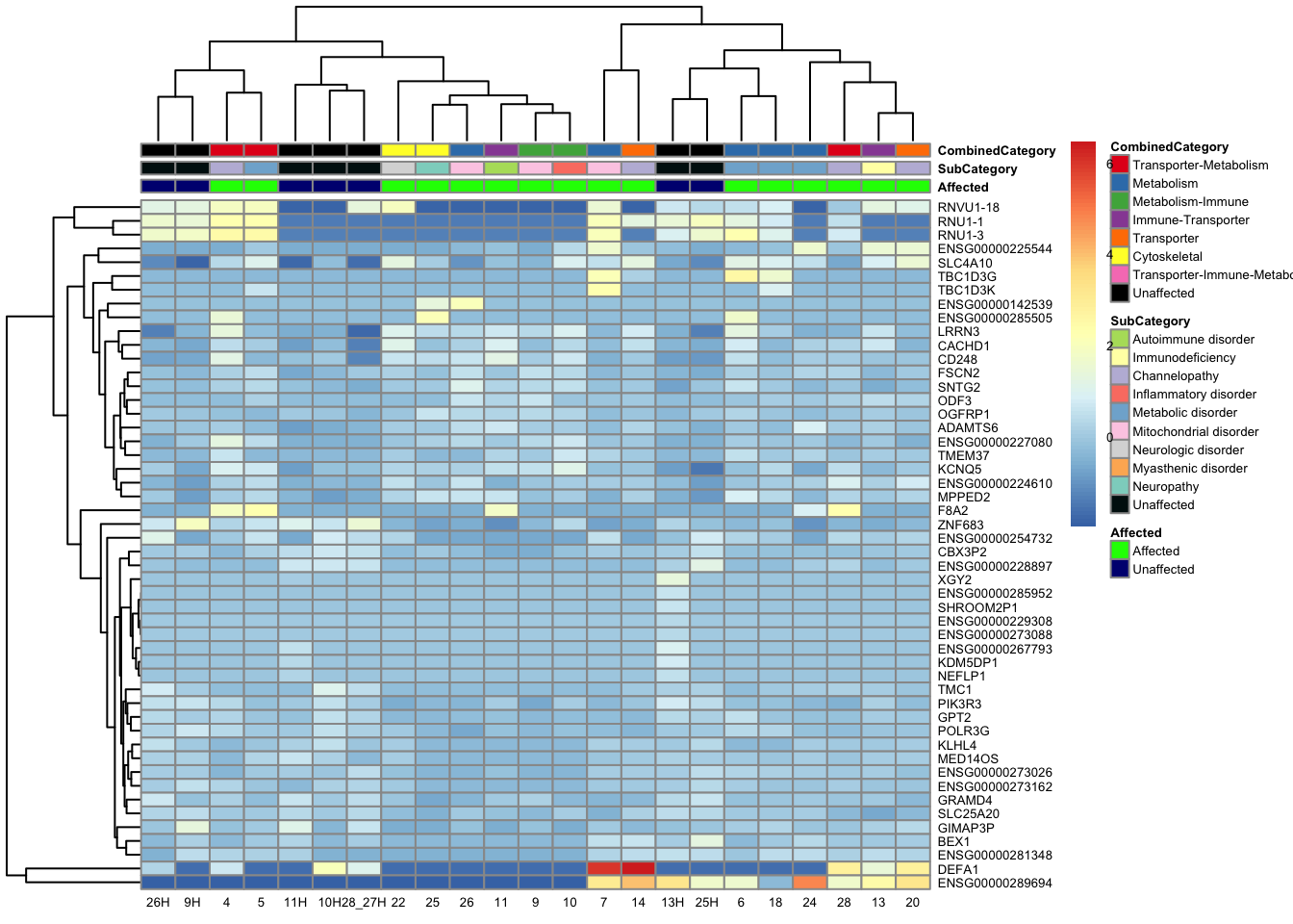
topgenes_byensemblid_sub <- head(rownames(res_aff_vs_unaff_df_sub), 55)
topgenes_aff_vs_unaff_05_sub <- assay(vsd_limma)[topgenes_byensemblid_sub, ]
topgenes_aff_vs_unaff_05_sub <- topgenes_aff_vs_unaff_05_sub - rowMeans(topgenes_aff_vs_unaff_05_sub)

ensembl_to_gene_sub <- setNames(gene_info$gene_name, gene_info$Ensembl_ID)

# Get the current row names of the matrix 'mat'
current_ensembl_ids_sub <- rownames(topgenes_aff_vs_unaff_05_sub)

# Find the corresponding gene names for the Ensembl IDs
new_row_names_sub <- ensembl_to_gene_sub[current_ensembl_ids_sub]

# Set the new row names for the matrix 'mat'
rownames(topgenes_aff_vs_unaff_05_sub) <- new_row_names_sub

topgenes_aff_vs_unaff_05_sub <- topgenes_aff_vs_unaff_05_sub[order(row.names(topgenes_aff_vs_unaff_05_sub)), ]

df_sub <- df <- colData(vsd_limma) %>%
  as.data.frame() %>%
  dplyr::select(CombinedCategory)
pheatmap(topgenes_aff_vs_unaff_05_sub, annotation_col = df_sub, annotation_colors = ann_colors2, fontsize = 5, angle_col = 0)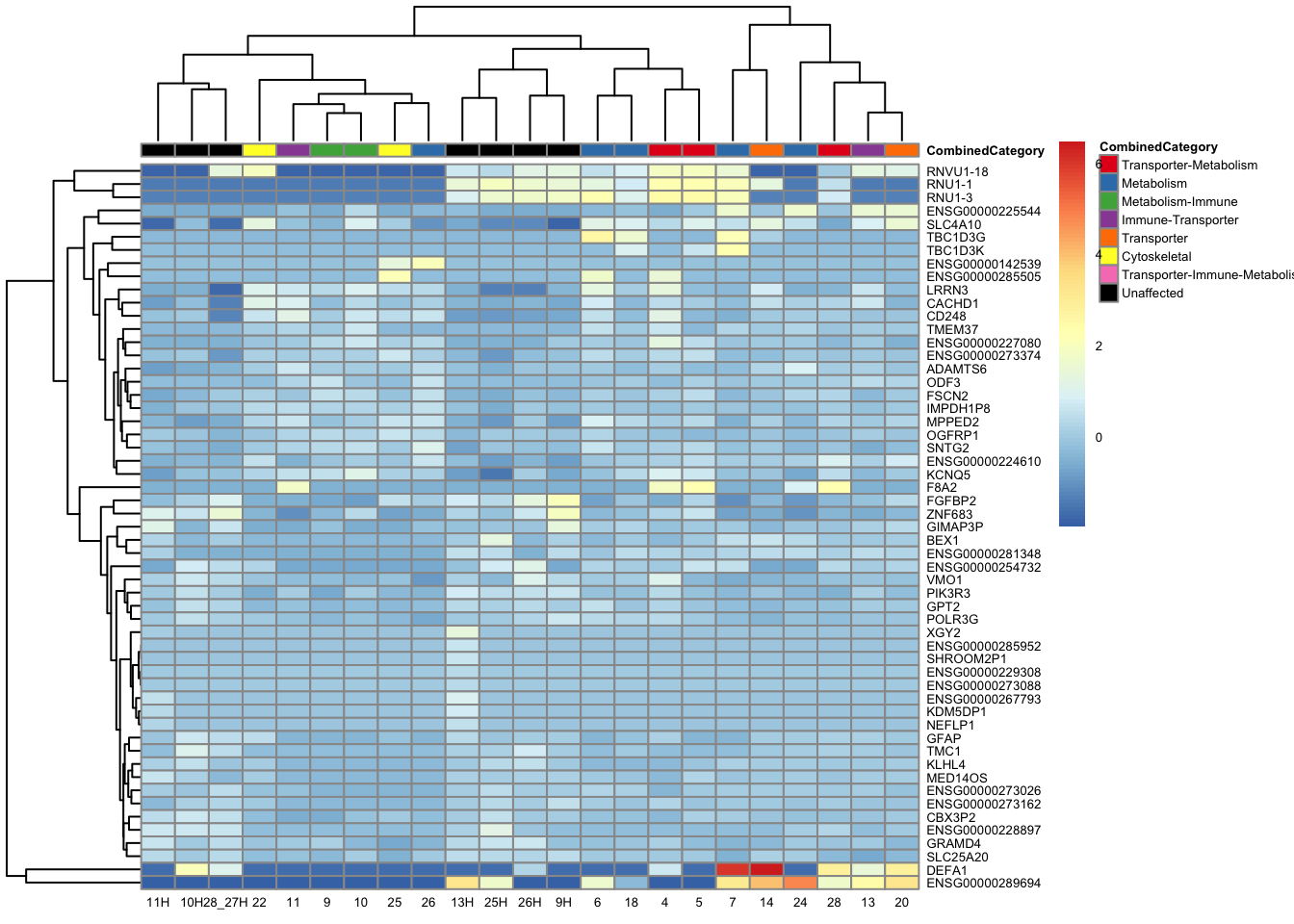
topgenes_byensemblid_sub <- head(rownames(res_aff_vs_unaff_df_sub), 55)
topgenes_aff_vs_unaff_05_sub <- assay(vsd_limma)[topgenes_byensemblid_sub, ]
topgenes_aff_vs_unaff_05_sub <- topgenes_aff_vs_unaff_05_sub - rowMeans(topgenes_aff_vs_unaff_05_sub)

ensembl_to_gene_sub <- setNames(gene_info$gene_name, gene_info$Ensembl_ID)

# Get the current row names of the matrix 'mat'
current_ensembl_ids_sub <- rownames(topgenes_aff_vs_unaff_05_sub)

# Find the corresponding gene names for the Ensembl IDs
new_row_names_sub <- ensembl_to_gene_sub[current_ensembl_ids_sub]

# Set the new row names for the matrix 'mat'
rownames(topgenes_aff_vs_unaff_05_sub) <- new_row_names_sub

topgenes_aff_vs_unaff_05_sub <- topgenes_aff_vs_unaff_05_sub[order(row.names(topgenes_aff_vs_unaff_05_sub)), ]

df_sub <- df <- colData(vsd_limma) %>%
  as.data.frame() %>%
  dplyr::select(Affected, SubCategory, CombinedCategory)
pheatmap(topgenes_aff_vs_unaff_05_sub, annotation_col = df_sub, annotation_colors = ann_colors2, fontsize = 5, angle_col = 0)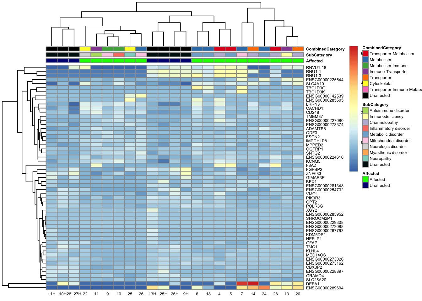
topgenes_byensemblid_sub <- head(rownames(res_aff_vs_unaff_df_sub), 75)
topgenes_aff_vs_unaff_05_sub <- assay(vsd_limma)[topgenes_byensemblid_sub, ]
topgenes_aff_vs_unaff_05_sub <- topgenes_aff_vs_unaff_05_sub - rowMeans(topgenes_aff_vs_unaff_05_sub)

ensembl_to_gene_sub <- setNames(gene_info$gene_name, gene_info$Ensembl_ID)

# Get the current row names of the matrix 'mat'
current_ensembl_ids_sub <- rownames(topgenes_aff_vs_unaff_05_sub)

# Find the corresponding gene names for the Ensembl IDs
new_row_names_sub <- ensembl_to_gene_sub[current_ensembl_ids_sub]

# Set the new row names for the matrix 'mat'
rownames(topgenes_aff_vs_unaff_05_sub) <- new_row_names_sub

topgenes_aff_vs_unaff_05_sub <- topgenes_aff_vs_unaff_05_sub[order(row.names(topgenes_aff_vs_unaff_05_sub)), ]

df_sub <- as.data.frame(colData(vsd_limma)[, c("Affected", "CombinedCategory")])
pheatmap(topgenes_aff_vs_unaff_05_sub, annotation_col = df_sub,
         annotation_colors = ann_colors2, fontsize = 4, angle_col = 0)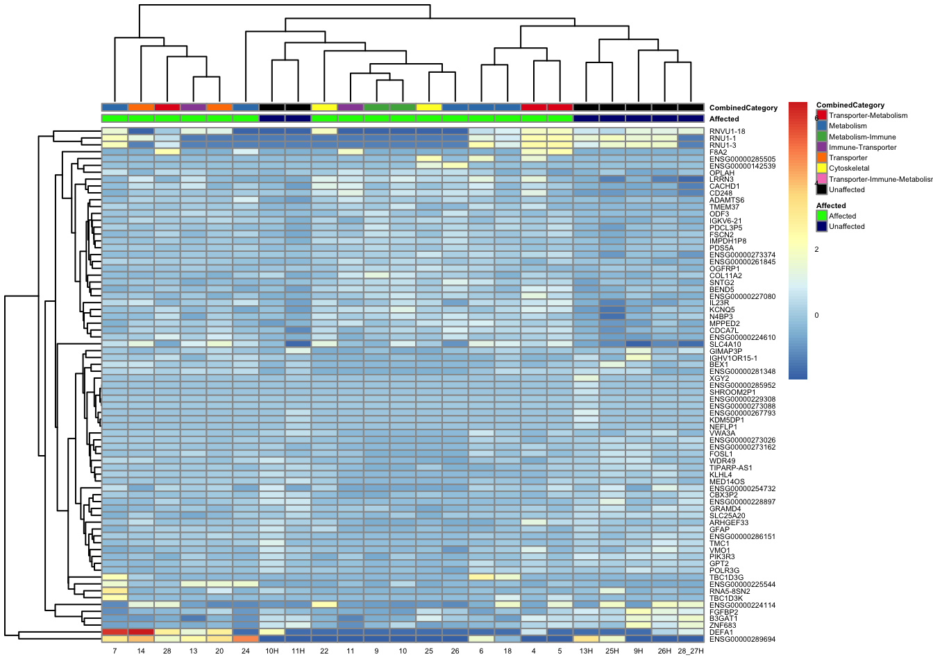
topgenes_byensemblid_sub <- head(rownames(res_aff_vs_unaff_df_sub), 75)
topgenes_aff_vs_unaff_05_sub <- assay(vsd_limma)[topgenes_byensemblid_sub, ]
topgenes_aff_vs_unaff_05_sub <- topgenes_aff_vs_unaff_05_sub - rowMeans(topgenes_aff_vs_unaff_05_sub)

ensembl_to_gene_sub <- setNames(gene_info$gene_name, gene_info$Ensembl_ID)

# Get the current row names of the matrix 'mat'
current_ensembl_ids_sub <- rownames(topgenes_aff_vs_unaff_05_sub)

# Find the corresponding gene names for the Ensembl IDs
new_row_names_sub <- ensembl_to_gene_sub[current_ensembl_ids_sub]

# Set the new row names for the matrix 'mat'
rownames(topgenes_aff_vs_unaff_05_sub) <- new_row_names_sub

topgenes_aff_vs_unaff_05_sub <- topgenes_aff_vs_unaff_05_sub[order(row.names(topgenes_aff_vs_unaff_05_sub)), ]

df_sub <- as.data.frame(colData(vsd_limma)[, c("Affected", "SubCategory", "CombinedCategory")])
pheatmap(topgenes_aff_vs_unaff_05_sub, annotation_col = df_sub, annotation_colors = ann_colors2, fontsize = 4, angle_col = 0)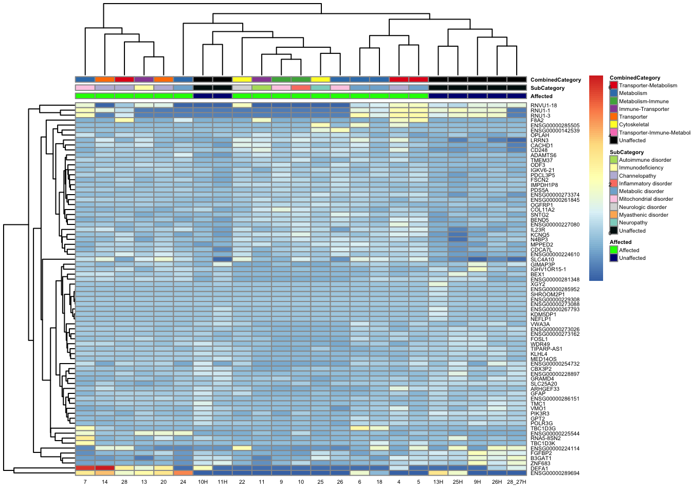
topgenes_byensemblid_sub <- head(rownames(res_aff_vs_unaff_df_sub), 200)
topgenes_aff_vs_unaff_05_sub <- assay(vsd_limma)[topgenes_byensemblid_sub, ]
topgenes_aff_vs_unaff_05_sub <- topgenes_aff_vs_unaff_05_sub - rowMeans(topgenes_aff_vs_unaff_05_sub)

ensembl_to_gene_sub <- setNames(gene_info$gene_name, gene_info$Ensembl_ID)

# Get the current row names of the matrix 'mat'
current_ensembl_ids_sub <- rownames(topgenes_aff_vs_unaff_05_sub)

# Find the corresponding gene names for the Ensembl IDs
new_row_names_sub <- ensembl_to_gene_sub[current_ensembl_ids_sub]

# Set the new row names for the matrix 'mat'
rownames(topgenes_aff_vs_unaff_05_sub) <- new_row_names_sub

topgenes_aff_vs_unaff_05_sub <- topgenes_aff_vs_unaff_05_sub[order(row.names(topgenes_aff_vs_unaff_05_sub)), ]

df_sub <- as.data.frame(colData(vsd_limma)[, c("Affected", "CombinedCategory")])
pheatmap(topgenes_aff_vs_unaff_05_sub, annotation_col = df_sub, annotation_colors = ann_colors2, fontsize = 2.25, angle_col = 0)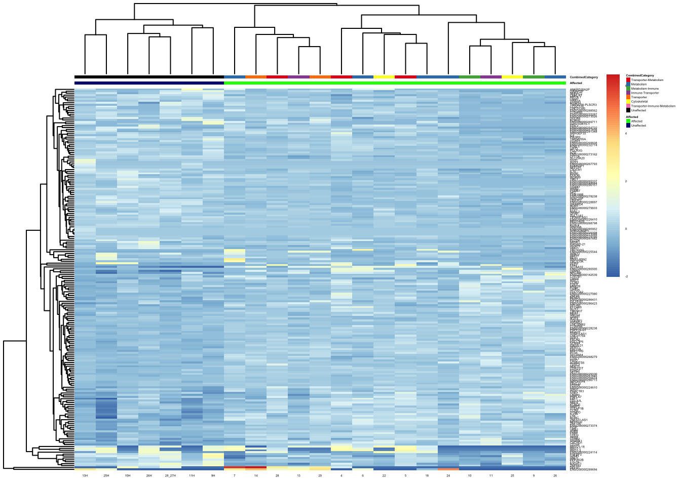
topgenes_byensemblid_sub <- head(rownames(res_aff_vs_unaff_df_sub), 200)
topgenes_aff_vs_unaff_05_sub <- assay(vsd_limma)[topgenes_byensemblid_sub, ]
topgenes_aff_vs_unaff_05_sub <- topgenes_aff_vs_unaff_05_sub - rowMeans(topgenes_aff_vs_unaff_05_sub)

ensembl_to_gene_sub <- setNames(gene_info$gene_name, gene_info$Ensembl_ID)

# Get the current row names of the matrix 'mat'
current_ensembl_ids_sub <- rownames(topgenes_aff_vs_unaff_05_sub)

# Find the corresponding gene names for the Ensembl IDs
new_row_names_sub <- ensembl_to_gene_sub[current_ensembl_ids_sub]

# Set the new row names for the matrix 'mat'
rownames(topgenes_aff_vs_unaff_05_sub) <- new_row_names_sub

topgenes_aff_vs_unaff_05_sub <- topgenes_aff_vs_unaff_05_sub[order(row.names(topgenes_aff_vs_unaff_05_sub)), ]

df_sub <- as.data.frame(colData(vsd_limma)[, c("Affected", "SubCategory", "CombinedCategory")])
pheatmap(topgenes_aff_vs_unaff_05_sub, annotation_col = df_sub, annotation_colors = ann_colors2, fontsize = 2.25, angle_col = 0)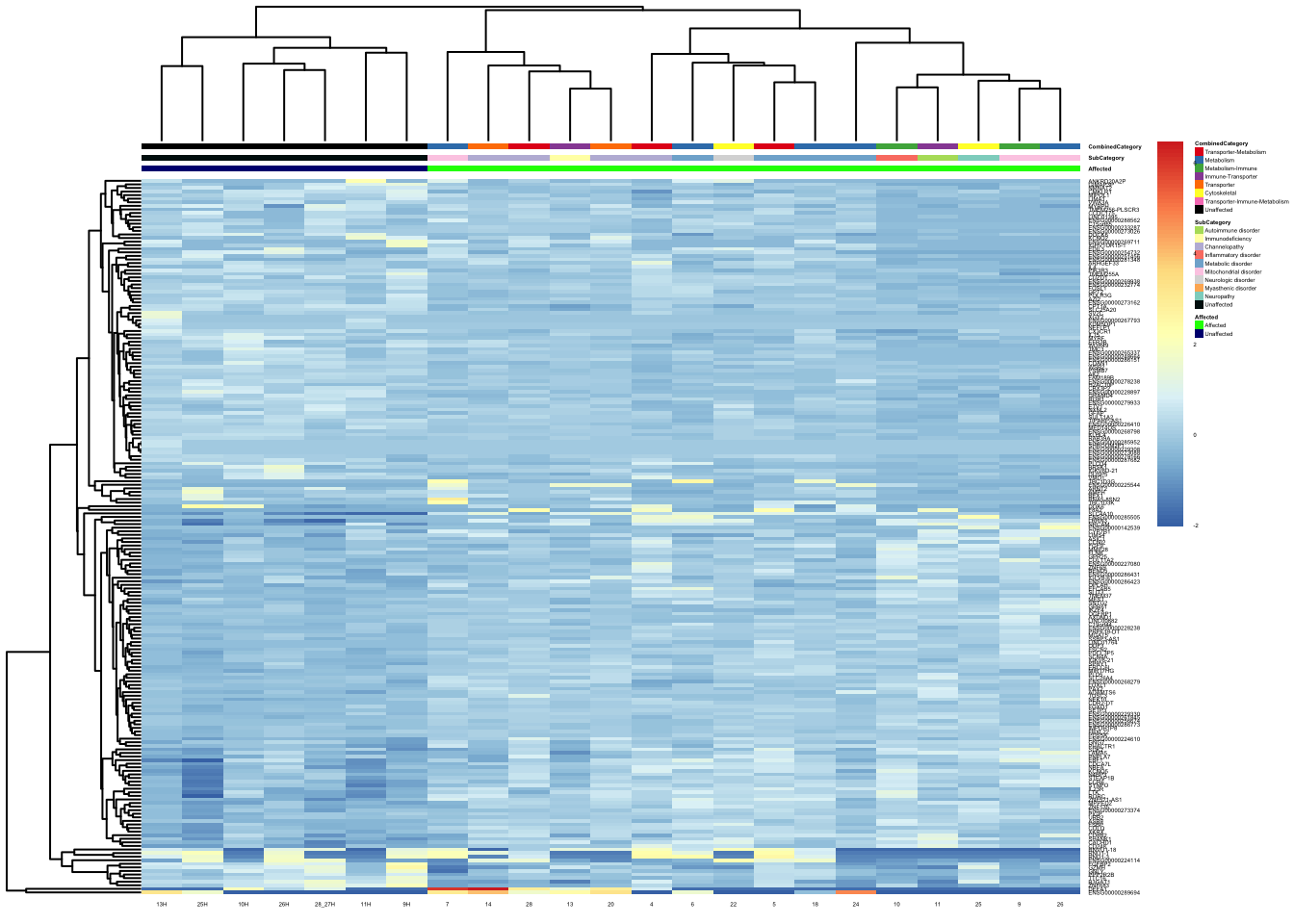
topgenes_byensemblid_sub <- head(rownames(res_aff_vs_unaff_df_sub), 125)
topgenes_aff_vs_unaff_05_sub <- assay(vsd_limma)[topgenes_byensemblid_sub, ]
topgenes_aff_vs_unaff_05_sub <- topgenes_aff_vs_unaff_05_sub - rowMeans(topgenes_aff_vs_unaff_05_sub)

ensembl_to_gene_sub <- setNames(gene_info$gene_name, gene_info$Ensembl_ID)

# Get the current row names of the matrix 'mat'
current_ensembl_ids_sub <- rownames(topgenes_aff_vs_unaff_05_sub)

# Find the corresponding gene names for the Ensembl IDs
new_row_names_sub <- ensembl_to_gene_sub[current_ensembl_ids_sub]

# Set the new row names for the matrix 'mat'
rownames(topgenes_aff_vs_unaff_05_sub) <- new_row_names_sub

# topgenes_aff_vs_unaff_05_sub <- topgenes_aff_vs_unaff_05_sub[order(row.names(topgenes_aff_vs_unaff_05_sub)), ]

df_sub <- as.data.frame(colData(vsd_limma)[, c("Affected", "CombinedCategory")])
pheatmap(topgenes_aff_vs_unaff_05_sub, annotation_col = df_sub, annotation_colors = ann_colors2, fontsize = 3.75, angle_col = 0)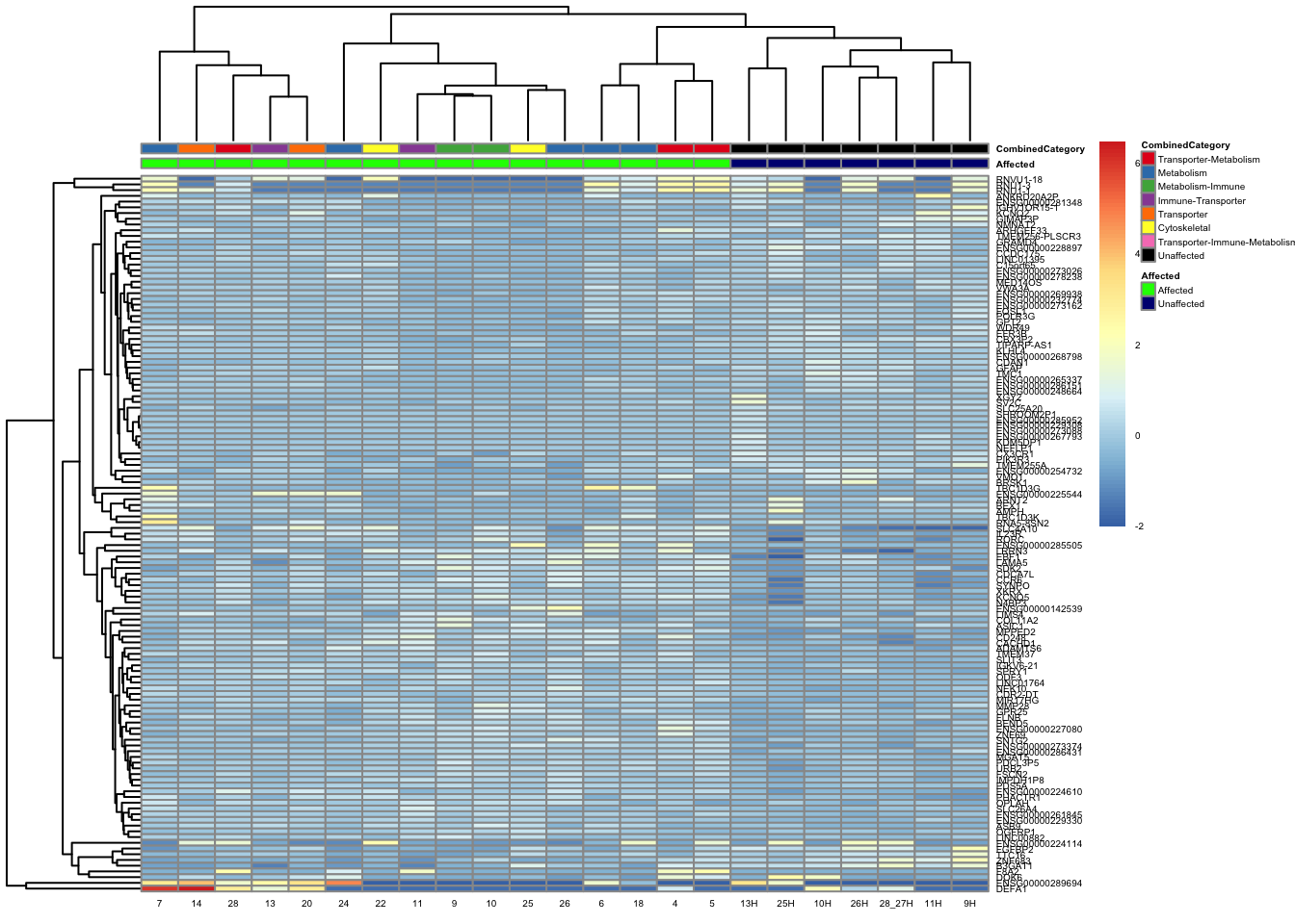
topgenes_byensemblid_sub <- head(rownames(res_aff_vs_unaff_df_sub), 125)
topgenes_aff_vs_unaff_05_sub <- assay(vsd_limma)[topgenes_byensemblid_sub, ]
topgenes_aff_vs_unaff_05_sub <- topgenes_aff_vs_unaff_05_sub - rowMeans(topgenes_aff_vs_unaff_05_sub)

ensembl_to_gene_sub <- setNames(gene_info$gene_name, gene_info$Ensembl_ID)

# Get the current row names of the matrix 'mat'
current_ensembl_ids_sub <- rownames(topgenes_aff_vs_unaff_05_sub)

# Find the corresponding gene names for the Ensembl IDs
new_row_names_sub <- ensembl_to_gene_sub[current_ensembl_ids_sub]

# Set the new row names for the matrix 'mat'
rownames(topgenes_aff_vs_unaff_05_sub) <- new_row_names_sub

# topgenes_aff_vs_unaff_05_sub <- topgenes_aff_vs_unaff_05_sub[order(row.names(topgenes_aff_vs_unaff_05_sub)), ]

df_sub <- as.data.frame(colData(vsd_limma)[, c("Affected", "SubCategory", "CombinedCategory")])
pheatmap(topgenes_aff_vs_unaff_05_sub, annotation_col = df_sub, annotation_colors = ann_colors2, fontsize = 3.75, angle_col = 0)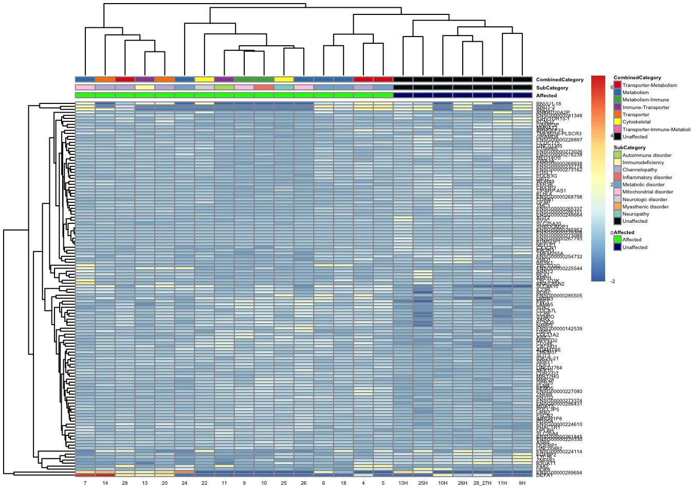
topgenes_byensemblid_sub <- head(rownames(res_aff_vs_unaff_df_sub), 150)
topgenes_aff_vs_unaff_05_sub <- assay(vsd_limma)[topgenes_byensemblid_sub, ]
topgenes_aff_vs_unaff_05_sub <- topgenes_aff_vs_unaff_05_sub - rowMeans(topgenes_aff_vs_unaff_05_sub)

ensembl_to_gene_sub <- setNames(gene_info$gene_name, gene_info$Ensembl_ID)

# Get the current row names of the matrix 'mat'
current_ensembl_ids_sub <- rownames(topgenes_aff_vs_unaff_05_sub)

# Find the corresponding gene names for the Ensembl IDs
new_row_names_sub <- ensembl_to_gene_sub[current_ensembl_ids_sub]

# Set the new row names for the matrix 'mat'
rownames(topgenes_aff_vs_unaff_05_sub) <- new_row_names_sub

# topgenes_aff_vs_unaff_05_sub <- topgenes_aff_vs_unaff_05_sub[order(row.names(topgenes_aff_vs_unaff_05_sub)), ]

df_sub <- as.data.frame(colData(vsd_limma)[, c("Affected", "CombinedCategory")])
pheatmap(topgenes_aff_vs_unaff_05_sub, annotation_col = df_sub, annotation_colors = ann_colors2, fontsize = 3.5, angle_col = 0)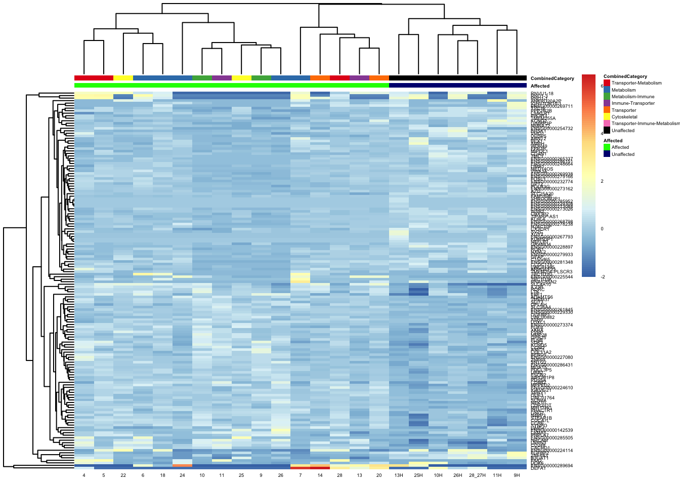
topgenes_byensemblid_sub <- head(rownames(res_aff_vs_unaff_df_sub), 150)
topgenes_aff_vs_unaff_05_sub <- assay(vsd_limma)[topgenes_byensemblid_sub, ]
topgenes_aff_vs_unaff_05_sub <- topgenes_aff_vs_unaff_05_sub - rowMeans(topgenes_aff_vs_unaff_05_sub)

ensembl_to_gene_sub <- setNames(gene_info$gene_name, gene_info$Ensembl_ID)

# Get the current row names of the matrix 'mat'
current_ensembl_ids_sub <- rownames(topgenes_aff_vs_unaff_05_sub)

# Find the corresponding gene names for the Ensembl IDs
new_row_names_sub <- ensembl_to_gene_sub[current_ensembl_ids_sub]

# Set the new row names for the matrix 'mat'
rownames(topgenes_aff_vs_unaff_05_sub) <- new_row_names_sub

# topgenes_aff_vs_unaff_05_sub <- topgenes_aff_vs_unaff_05_sub[order(row.names(topgenes_aff_vs_unaff_05_sub)), ]

df_sub <- as.data.frame(colData(vsd_limma)[, c("Affected", "SubCategory", "CombinedCategory")])
pheatmap(topgenes_aff_vs_unaff_05_sub, annotation_col = df_sub, annotation_colors = ann_colors2, fontsize = 3.5, angle_col = 0)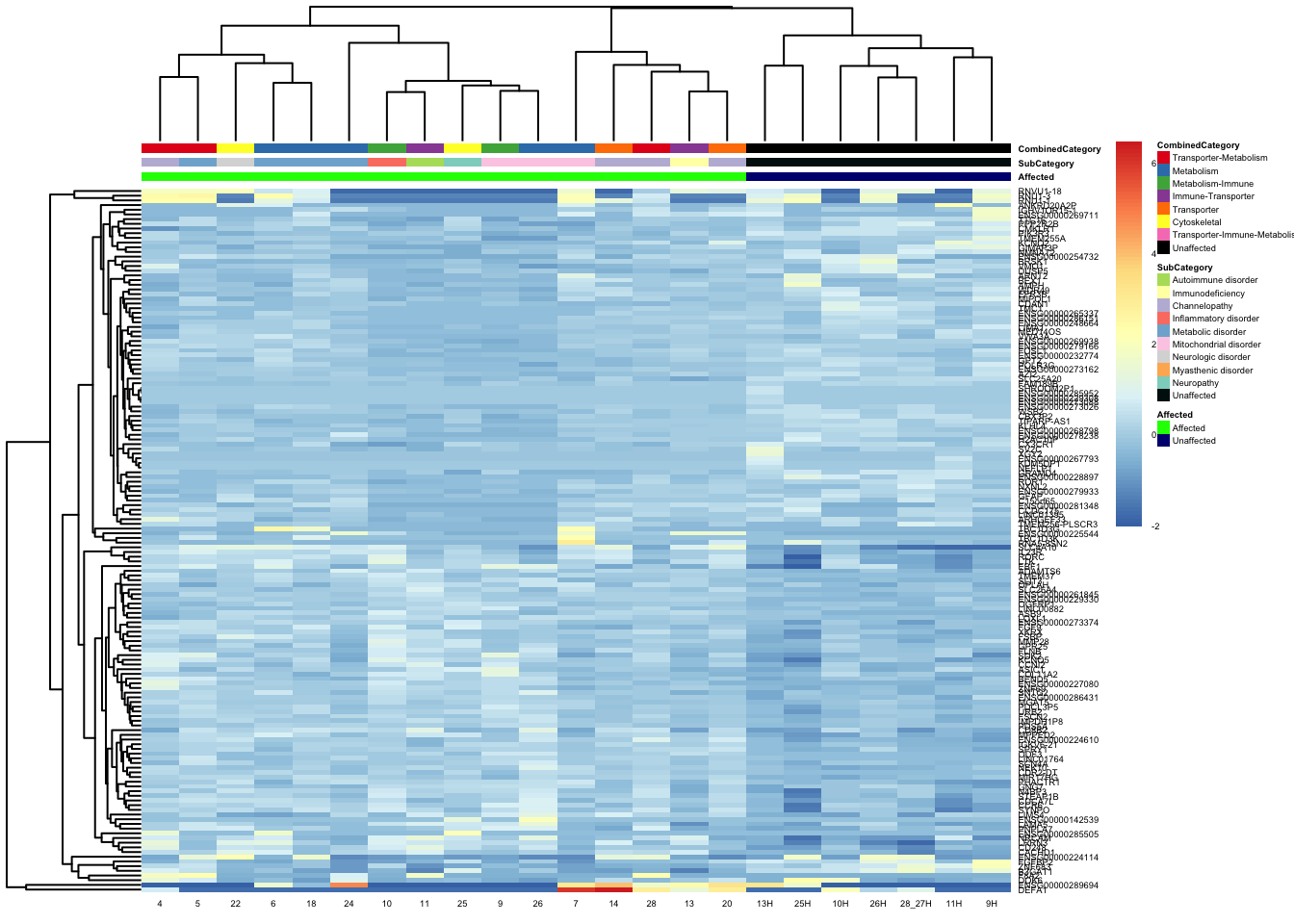
gb_df <- genes_biomart[, c(1, ncol(genes_biomart))]
res_aff_vs_unaff_df_sub_genename <- res_aff_vs_unaff_df_sub
res_aff_vs_unaff_df_sub_genename$Ensembl_ID <- row.names(res_aff_vs_unaff_df_sub)
res_aff_vs_unaff_df_sub_genename <- merge(x = res_aff_vs_unaff_df_sub_genename, y = gene_info, by.x = "Ensembl_ID", by.y = "Ensembl_ID", all.x = TRUE)
res_aff_vs_unaff_df_sub_genename <- res_aff_vs_unaff_df_sub_genename[, c(dim(res_aff_vs_unaff_df_sub_genename)[2], 1:dim(res_aff_vs_unaff_df_sub_genename)[2] - 1)]
res_aff_vs_unaff_df_sub_genename <- res_aff_vs_unaff_df_sub_genename[order(res_aff_vs_unaff_df_sub_genename[, "padj"]), ]
write.csv(res_aff_vs_unaff_df_sub_genename, file = "output/res_aff_vs_unaff_df_sub_genename.csv")
res_aff_vs_unaff_df_genename_05 <- subset(res_aff_vs_unaff_df_sub_genename, padj < 0.05)
res_aff_vs_unaff_df_genename_05 <- res_aff_vs_unaff_df_genename_05[order(res_aff_vs_unaff_df_genename_05$padj), ]
write.csv(res_aff_vs_unaff_df_genename_05, file = "output/res_aff_vs_unaff_df_sub_genename_05.csv")
res_aff_vs_unaff_df_genename_1 <- subset(res_aff_vs_unaff_df_sub_genename, padj < 0.1)
res_aff_vs_unaff_df_genename_1 <- res_aff_vs_unaff_df_genename_1[order(res_aff_vs_unaff_df_genename_1$padj), ]
write.csv(res_aff_vs_unaff_df_genename_1, file = "output/res_aff_vs_unaff_df_sub_genename_padj1.csv")Below is a table of information about the top genes.
library(mygene)

genes <- res_aff_vs_unaff_df_genename_05$gene_name
my_gene_data <- queryMany(genes, scopes = "symbol", fields = c("symbol", "name", "summary", species = "human"))
Finished
Pass returnall=TRUE to return lists of duplicate or missing query terms.my_gene_data_unique <- as.data.frame(my_gene_data) %>% dplyr::distinct(query, .keep_all = TRUE)
# paged_table(my_gene_data, options = list(rows.print = 15))filtered_gene_names <- res_aff_vs_unaff_df_sub_genename$gene_name[!grepl("^ENS", res_aff_vs_unaff_df_sub_genename$gene_name)]
# Select specific genes to show
# set top = 0, then specify genes using label.select argument
maplot <- ggmaplot(res_aff_vs_unaff_df_sub,
main = "Affected vs Unaffected MA Plot",
fdr = .1, fc = 1, size = 0.4, # Same used for others.
genenames = as.vector(res_aff_vs_unaff_df_sub_genename$gene_name),
ggtheme = ggplot2::theme_minimal(),
legend = "top", top = 30,
label.select = c("KCNQ5"),
font.label = c("bold", 6), label.rectangle = TRUE,
font.legend = "bold", font.main = "bold"
)
maplot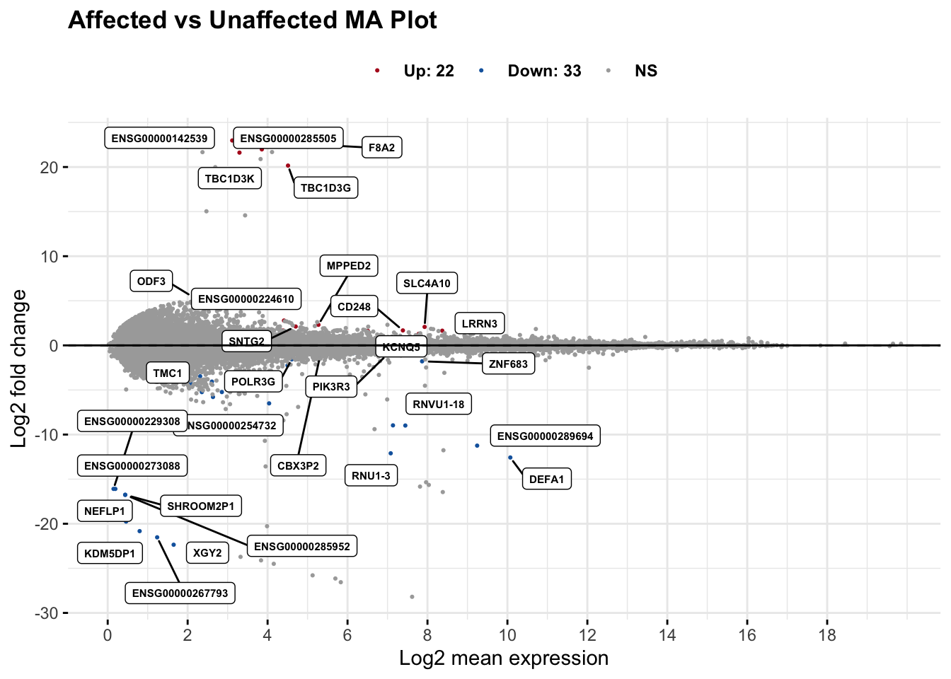
significant_data <- maplot$data %>%
  filter(grepl("Up|Down", sig)) %>%
  mutate(direction = ifelse(grepl("Up", sig), "Up", "Down")) %>%
  dplyr::select(-sig) # This removes the 'sig' column

# Combine DataFrames based on matching 'query' in my_gene_data_unique to 'gene' in significant_data
combined_data <- inner_join(my_gene_data_unique, significant_data, by = c("query" = "name"))

combined_data <- combined_data %>%
  dplyr::select(-notfound, -X_id, -X_score) %>%
  rename(gene = query)

paged_table(as.data.frame(significant_data), options = list(rows.print = 30))
# Save significant genes
write.csv(significant_data, file = "output/res_aff_vs_unaff_significant_subsetted_samples.csv", row.names = FALSE)
# Save significant genes
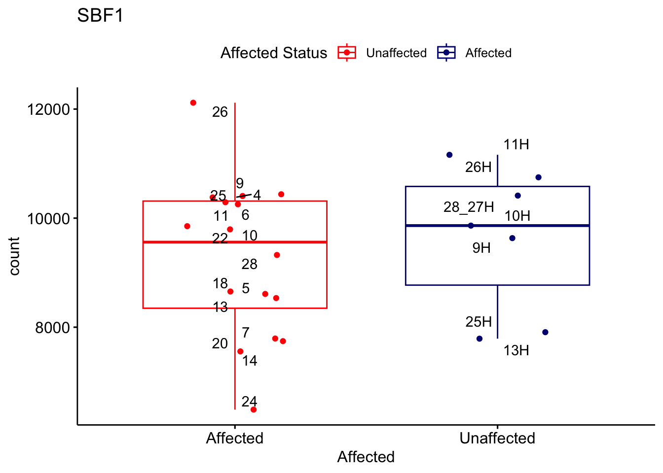
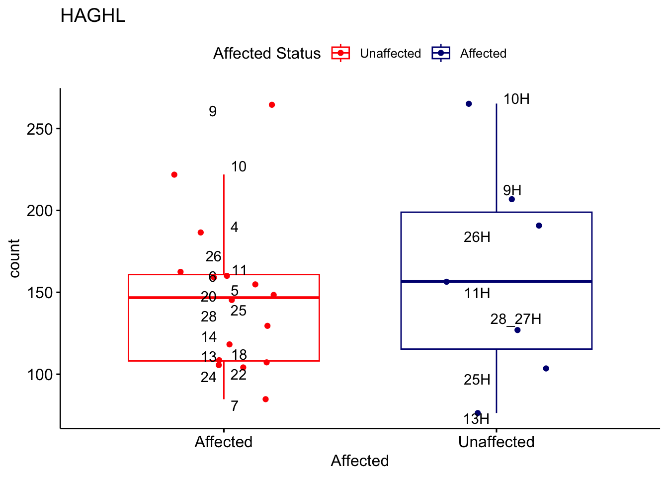
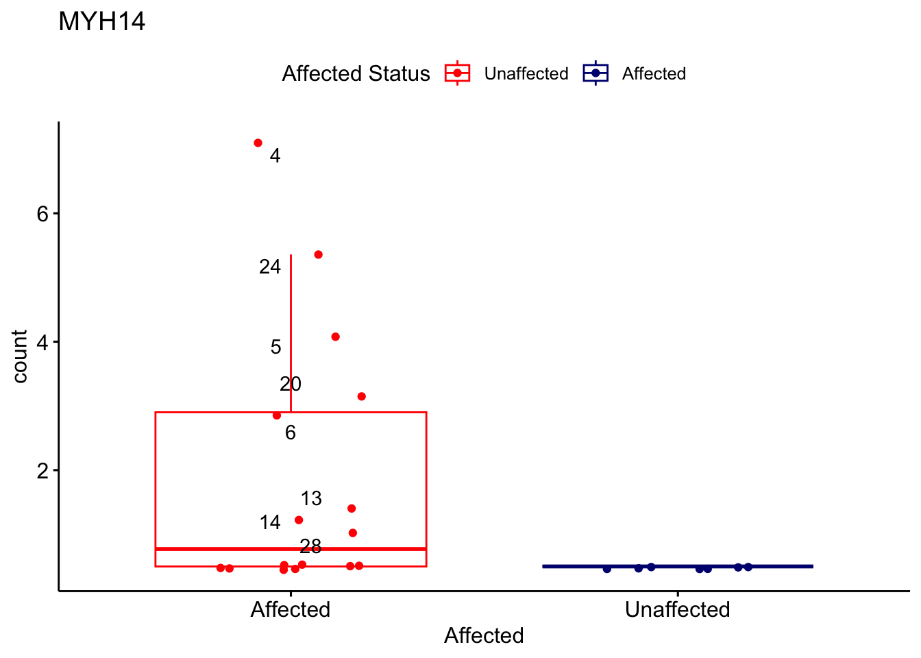
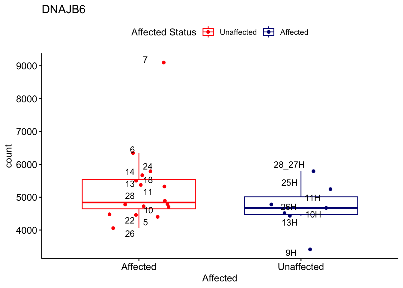
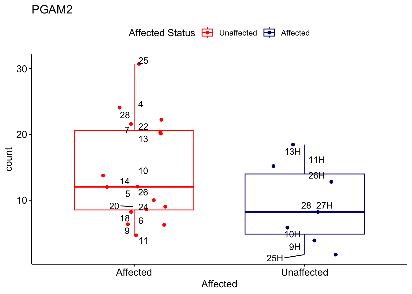
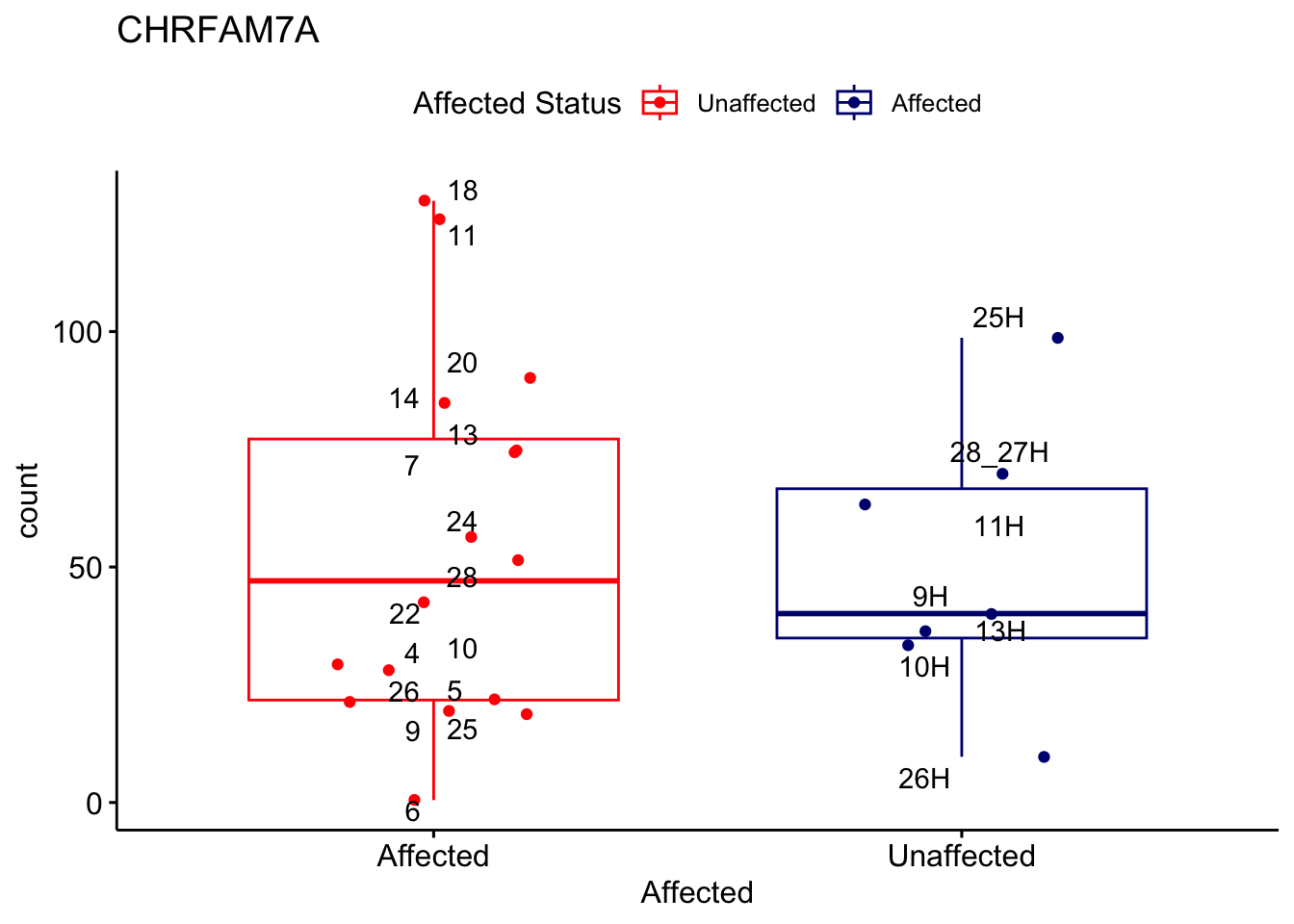
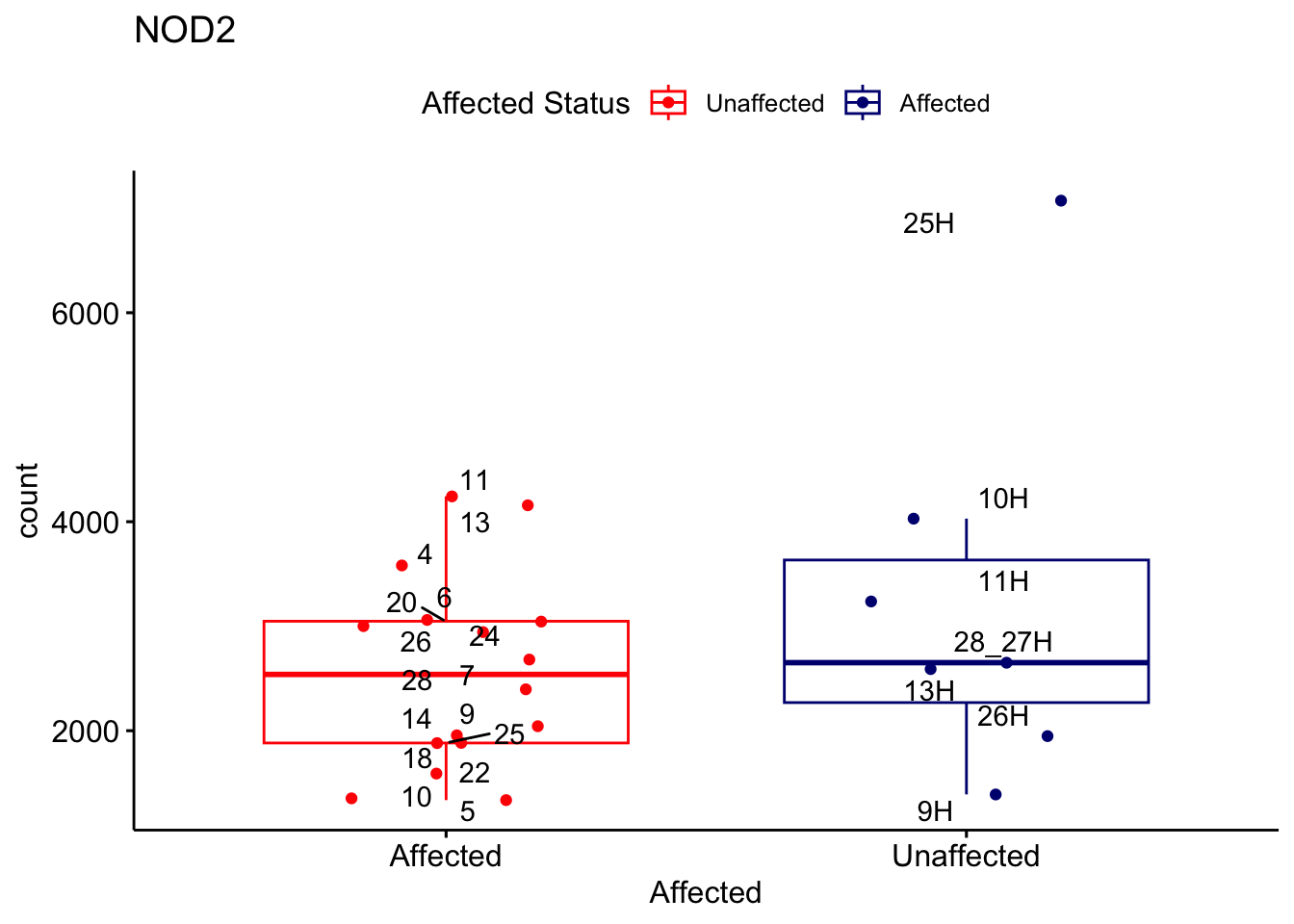
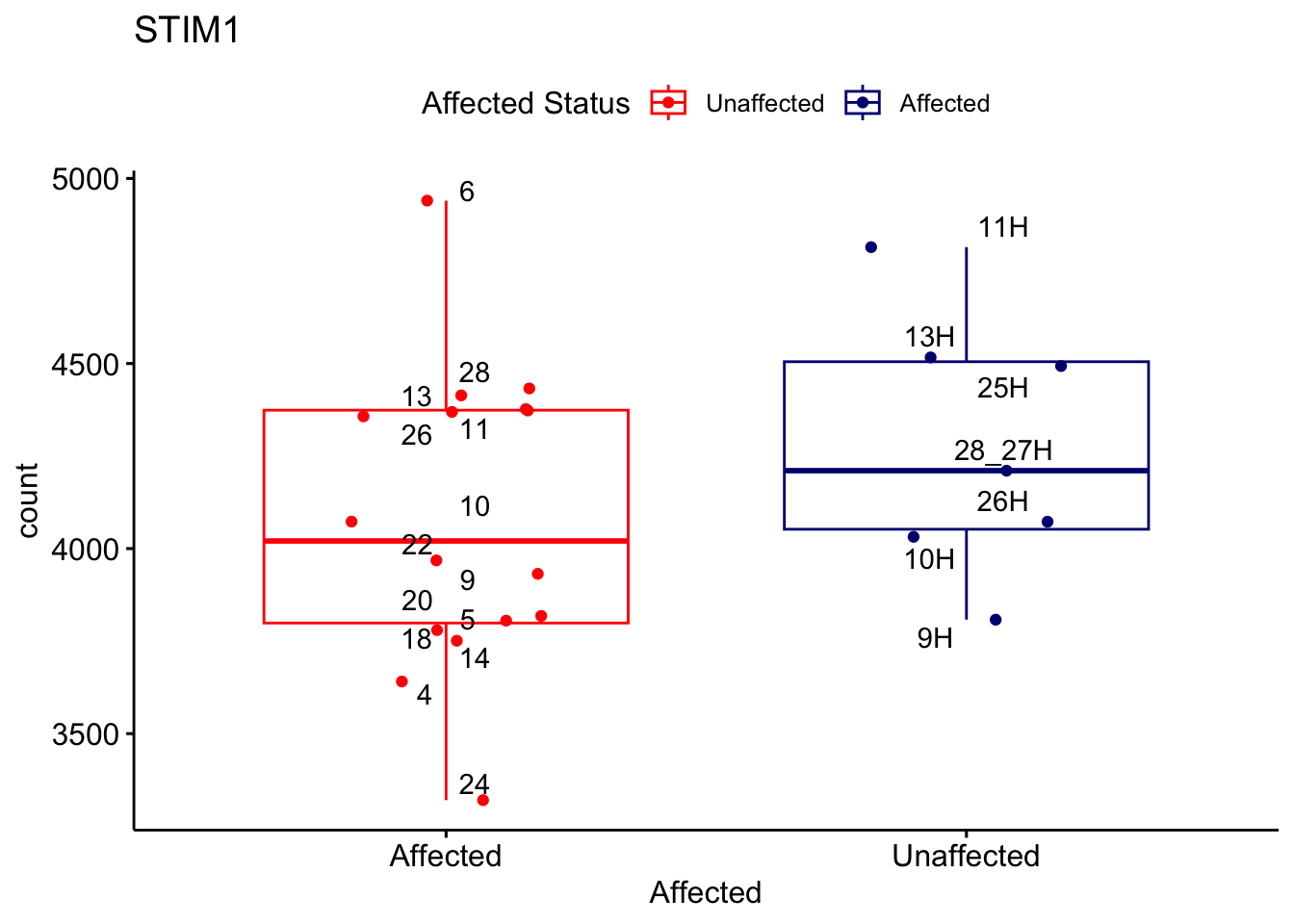
write.csv(combined_data, file = "output/res_aff_vs_unaff_significant_subsetted_mygene.csv", row.names = FALSE)Expression of Candidate Genes
Below is a table of expression of the genes identified during our WGS analysis.
8 of the genes were not included using DESeq2’s count filtering method (these genes had no counts):
“DPEP1”, “RERGL”, “TDO2”, “CCDC178”, “ADRA1D”, “AVPR1B”, “LRCOL1”, “KCNJ18”
# Subset gene_info using genes of interest
subset_gene_info <- gene_info[gene_info$gene_name %in% genes_of_interest, ]

filtered_by_interest <- filter(res_aff_vs_unaff_df_sub_genename, Ensembl_ID %in% subset_gene_info$Ensembl_ID)

# Filtering the dataframe by row names
filtered_counts <- counts[row.names(counts) %in% subset_gene_info$Ensembl_ID, ]

# Match and update row names
matching_indices <- match(rownames(filtered_counts), subset_gene_info$Ensembl_ID)

# Update row names based on matching_column values from metadata
rownames(filtered_counts) <- subset_gene_info$gene_name[matching_indices]

missing_genes <- setdiff(subset_gene_info$Ensembl_ID, filtered_by_interest$Ensembl_ID)

corresponding_gene_names <- subset_gene_info$gene_name[subset_gene_info$Ensembl_ID %in% missing_genes]

missing_gene_counts <- counts[row.names(counts) %in% missing_genes, ]

paged_table(filtered_by_interest, options = list(rows.print = 15))
paged_table(filtered_counts, options = list(rows.print = 15))Below is a heatmap highlighting the expression of our genes of interest across batch, disease group, and affected status.
mat3 <- assay(vsd_limma)[filtered_by_interest$Ensembl_ID, ]
rownames(mat3) <- gene_info$gene_name[match(filtered_by_interest$Ensembl_ID, gene_info$Ensembl_ID)]
df_sub <- as.data.frame(colData(vsd_limma)[, c("Affected", "CombinedCategory")])
pheatmap(mat3, annotation_col = df_sub, annotation_colors = ann_colors2, fontsize = 4, angle_col = 0)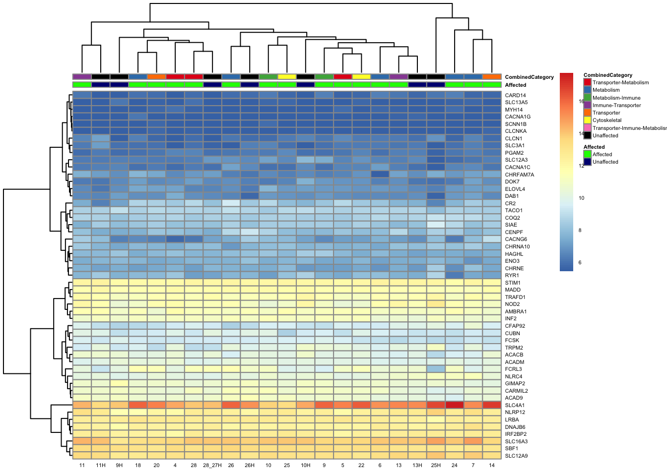
Enrichment analysis
res <- gost(query = significant_data$name, organism = "hsapiens", significant = FALSE) # should significant be true or false?

x <- gostplot(res, capped = FALSE, interactive = FALSE)
x + geom_label_repel(aes(label = "term_id"),
                  box.padding   = 0.35,
                  point.padding = 0.5,
                  segment.color = 'grey50')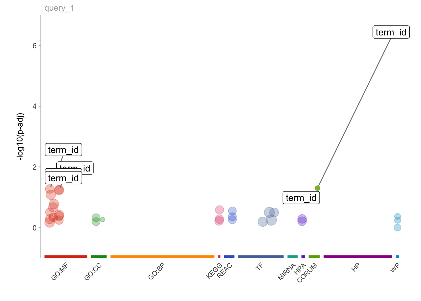
# Your existing code for obtaining geneList with Ensembl IDs
rownames(res_aff_vs_unaff_df_sub) <- gsub("\\..*", "", rownames(res_aff_vs_unaff_df_sub))
res_aff_vs_unaff_df_sub <- res_aff_vs_unaff_df_sub %>% dplyr::distinct()
geneList <- res_aff_vs_unaff_df_sub$log2FoldChange
names(geneList) <- rownames(res_aff_vs_unaff_df_sub)

# Initialize BioMart
ensembl <- useMart("ensembl", dataset = "hsapiens_gene_ensembl")

# Convert all Ensembl IDs in geneList to Entrez IDs
attributes <- c("ensembl_gene_id", "entrezgene_id")
filters <- "ensembl_gene_id"
results <- getBM(attributes = attributes, filters = filters, values = names(geneList), mart = ensembl)

# Remove rows with NA or empty Entrez IDs
results <- results[!is.na(results$entrezgene_id) & results$entrezgene_id != "", ]

# Create a new geneList with Entrez IDs
geneList_entrez <- geneList[results$ensembl_gene_id]
names(geneList_entrez) <- results$entrezgene_id

# Filter genes with abs(log2FoldChange) > 2
gene_entrez <- names(geneList_entrez)[abs(geneList_entrez) > 2]

# Run enrichGO with Entrez IDs
ego_cc <- enrichGO(
  gene = gene_entrez,
  universe = names(geneList_entrez),
  OrgDb = org.Hs.eg.db,
  ont = "CC",
  pAdjustMethod = "BH",
  pvalueCutoff = 0.01,
  qvalueCutoff = 0.05,
  readable = TRUE
)

# Plot results
dotplot(ego_cc, showCategory = 10, title = "Overrepresented Cellular Components") + ggthemes::theme_clean()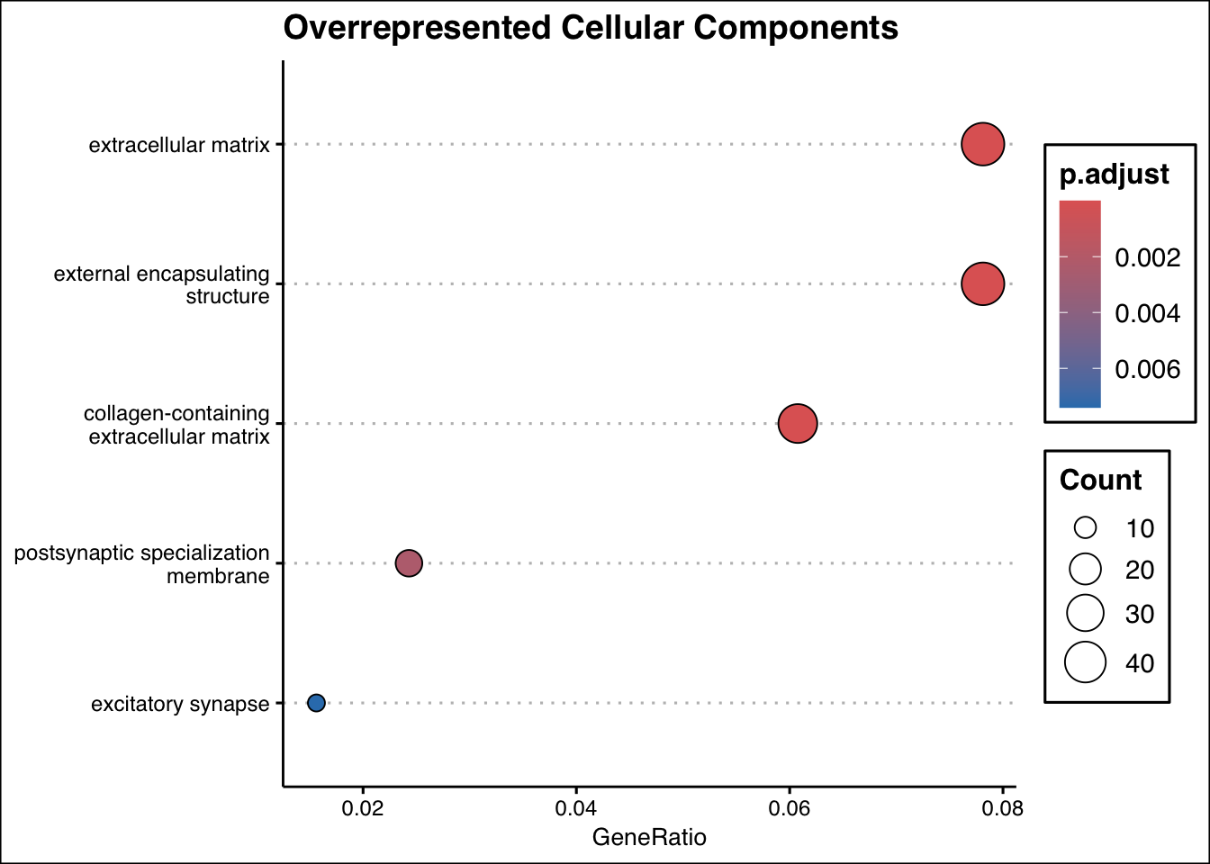
| Version | Author | Date |
|---|---|---|
| 1e45c53 | sdhutchins | 2024-04-09 |
ego_bp <- enrichGO(
  gene = gene_entrez,
  universe = names(geneList_entrez),
  OrgDb = org.Hs.eg.db,
  ont = "BP",
  pAdjustMethod = "BH",
  pvalueCutoff = 0.01,
  qvalueCutoff = 0.05,
  readable = TRUE
)

# Plot results
dotplot(ego_bp, showCategory = 10, title = "Overrepresented Biological Processes") + ggthemes::theme_clean()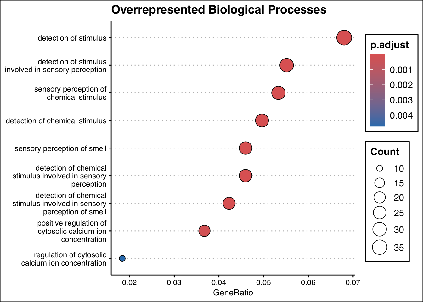
| Version | Author | Date |
|---|---|---|
| 1e45c53 | sdhutchins | 2024-04-09 |
ego_mf <- enrichGO(
  gene = gene_entrez,
  universe = names(geneList_entrez),
  OrgDb = org.Hs.eg.db,
  ont = "MF",
  pAdjustMethod = "BH",
  pvalueCutoff = 0.01,
  qvalueCutoff = 0.05,
  readable = TRUE
)

# Plot results
dotplot(ego_mf, showCategory = 10, title = "Overrepresented Molecular Functions") + ggthemes::theme_clean()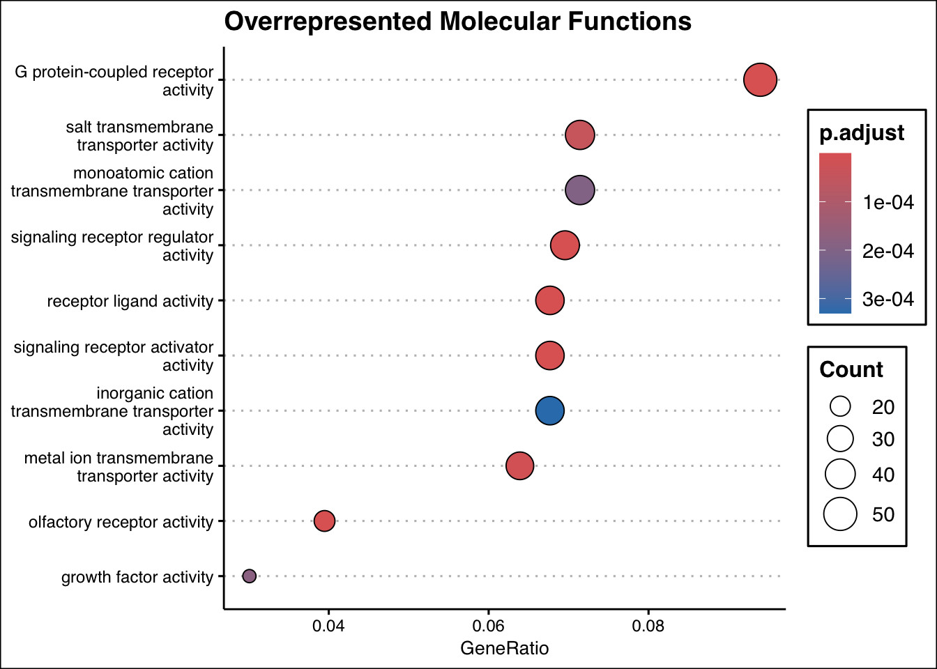
| Version | Author | Date |
|---|---|---|
| 1e45c53 | sdhutchins | 2024-04-09 |
library(DOSE)
gl <- geneList_entrez[abs(geneList_entrez) > 2]
gl <- na.omit(gl)
gl_sorted <- sort(gl, decreasing = TRUE)

gse <- gseGO(geneList     = gl_sorted,
              OrgDb        = org.Hs.eg.db,
              ont          = "ALL",
              minGSSize    = 3,
              maxGSSize    = 500,
              pvalueCutoff = 0.05,
              verbose      = FALSE)

dotplot(gse, showCategory = 10, split = ".sign", title = "GO Gene Set Enrichment Analysis") + facet_grid(.~.sign)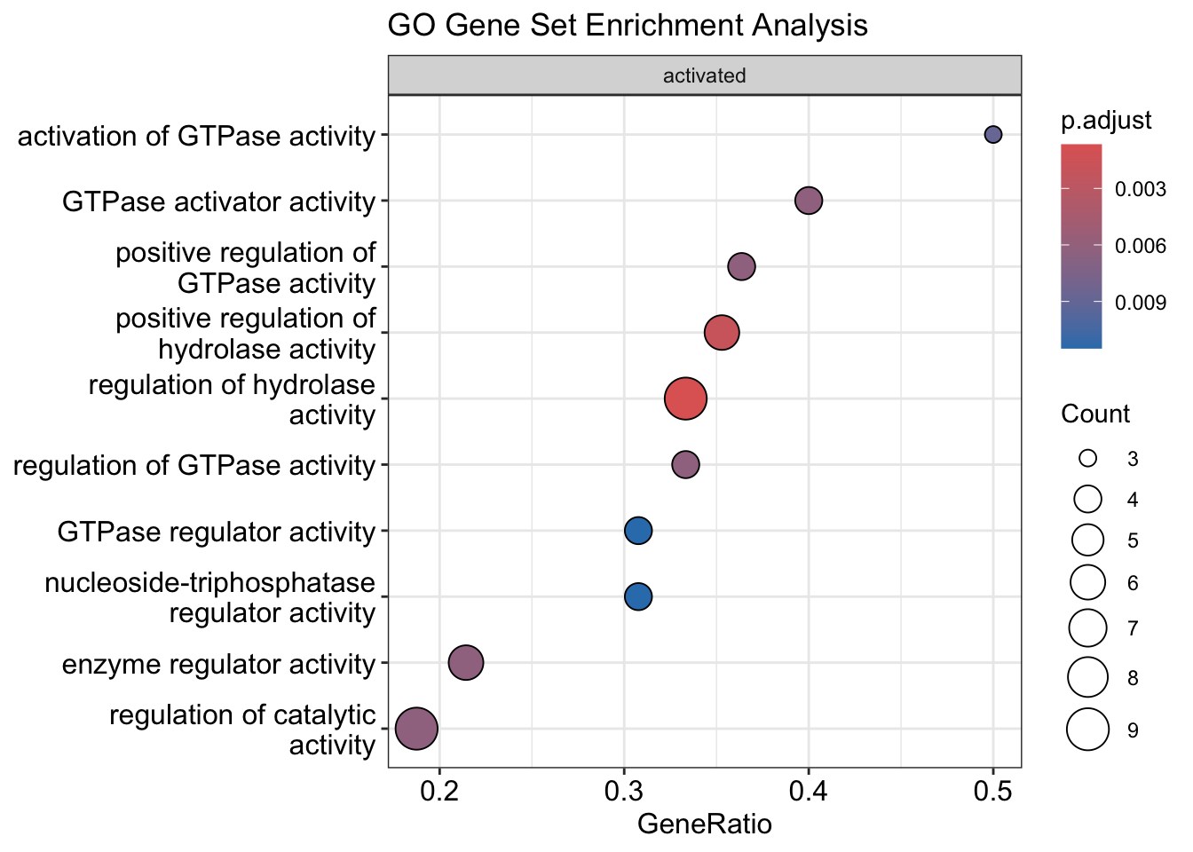
| Version | Author | Date |
|---|---|---|
| 1e45c53 | sdhutchins | 2024-04-09 |
kk2 <- gseKEGG(geneList     = gl_sorted,
               organism     = "hsa", # humans = hsa for KEGG
               nPerm        = 100000,
               minGSSize    = 3,
               maxGSSize    = 800,
               pvalueCutoff = 0.05,
               pAdjustMethod = "none",
               keyType       = "ncbi-geneid")

dotplot(kk2, showCategory = 10, title = "Enriched KEGG Pathways" , split=".sign") + facet_grid(.~.sign)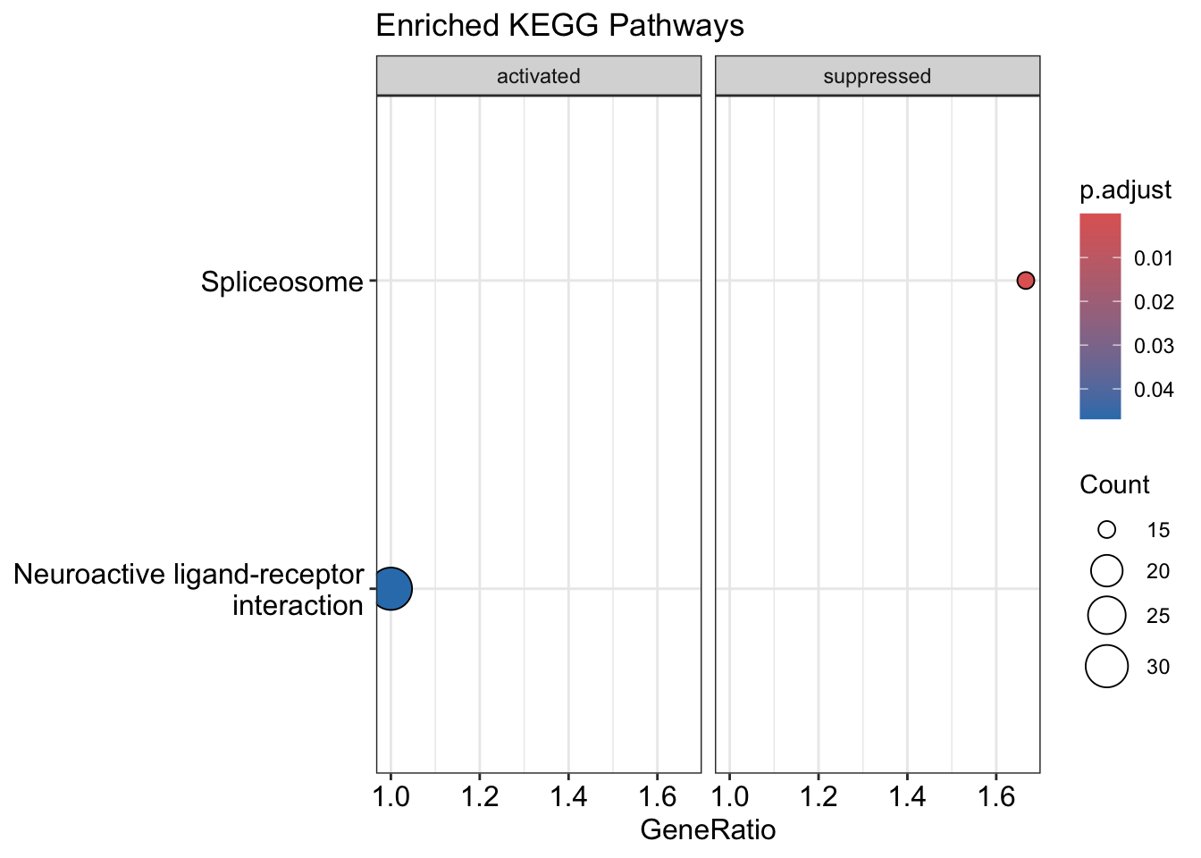
| Version | Author | Date |
|---|---|---|
| 1e45c53 | sdhutchins | 2024-04-09 |
y <- enrichPathway(gene_entrez, pvalueCutoff = 0.05)

dotplot(y, showCategory = 10, title = "Reactome Pathway Over-representation Analysis", font.size = 10) 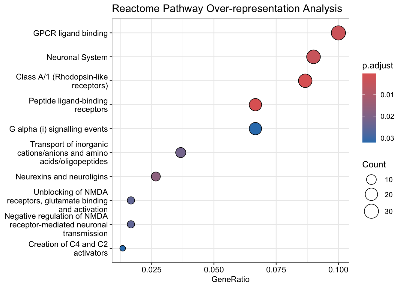
| Version | Author | Date |
|---|---|---|
| 1e45c53 | sdhutchins | 2024-04-09 |
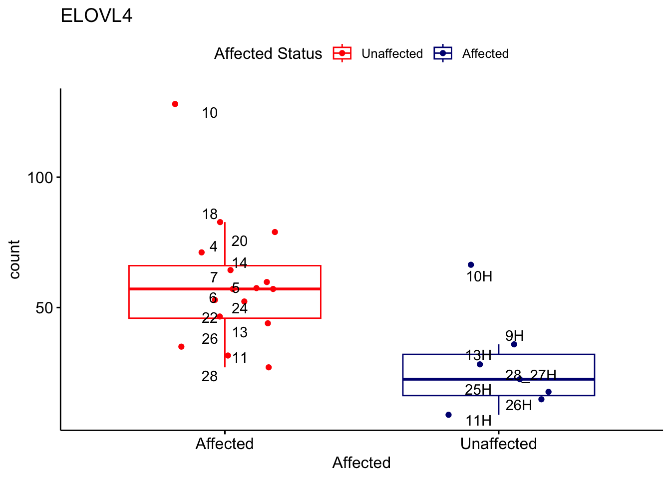
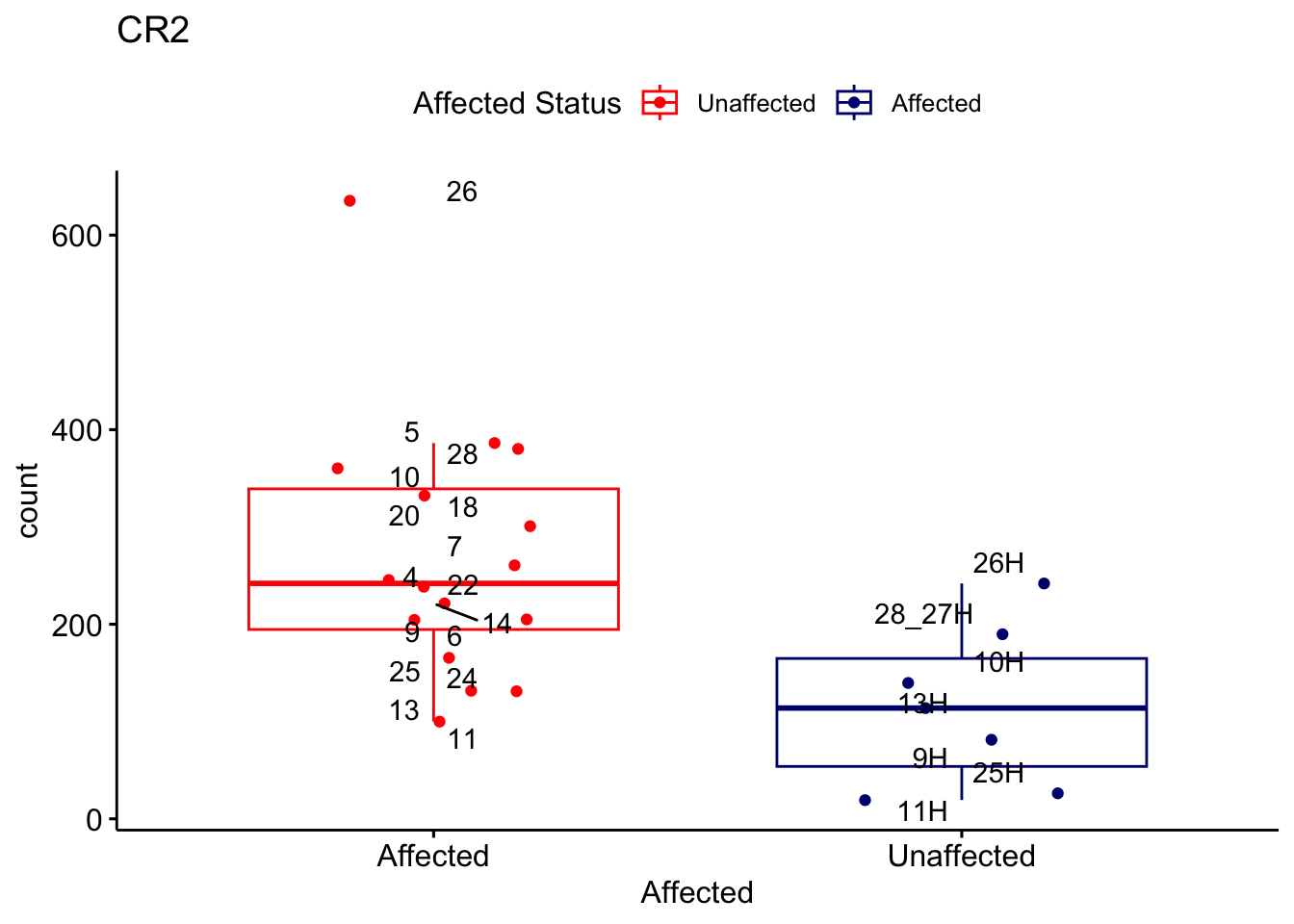
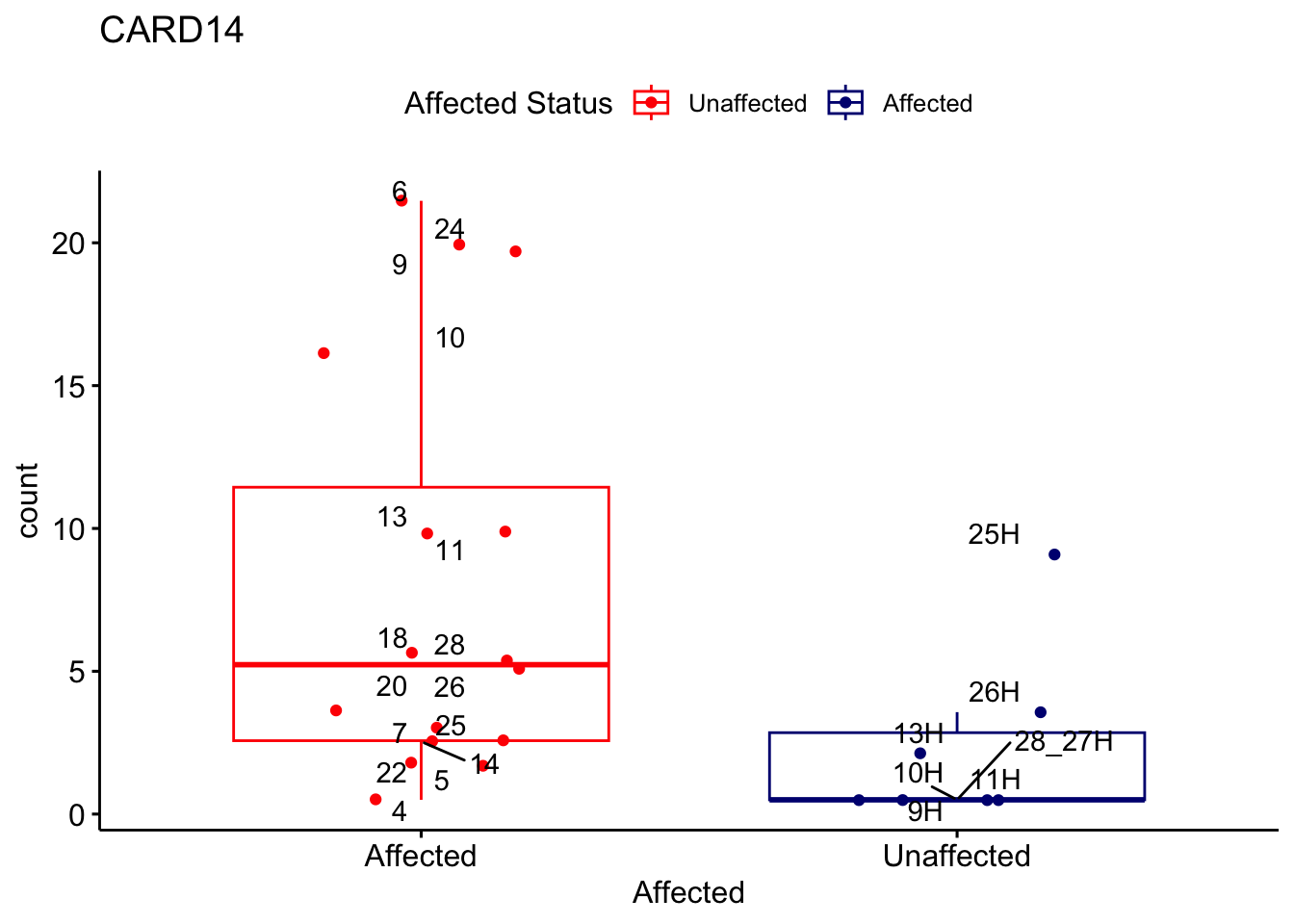
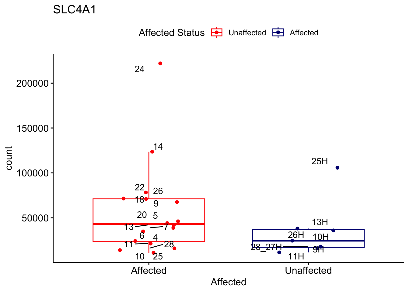
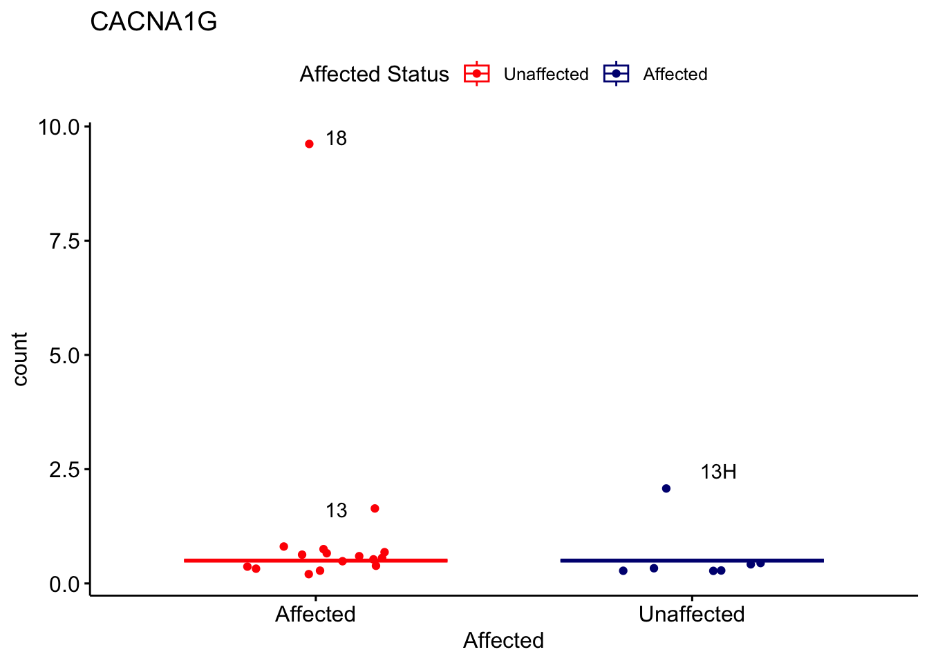
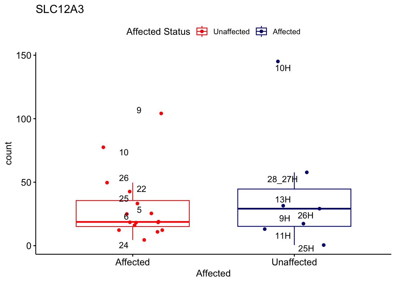
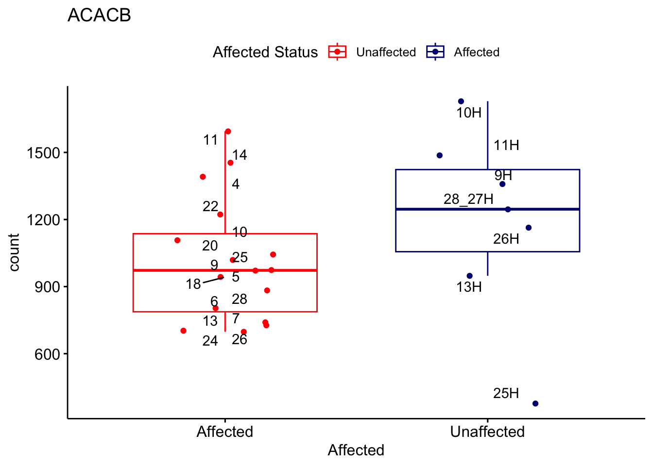
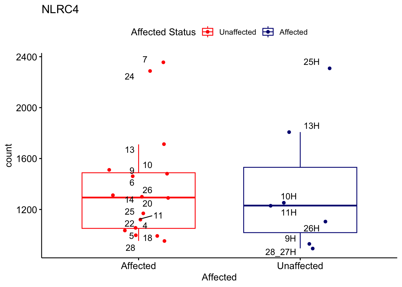
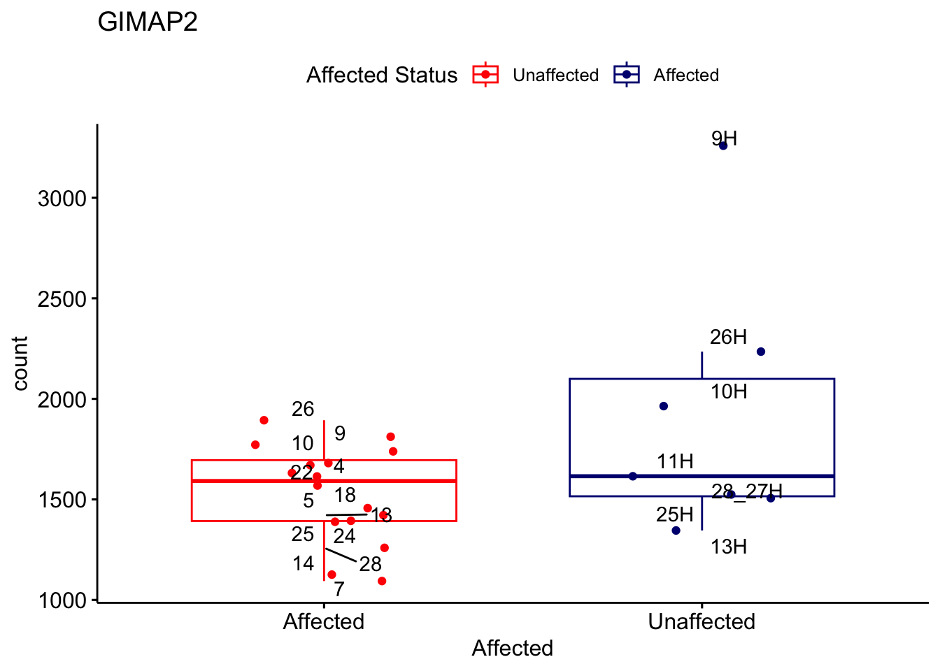
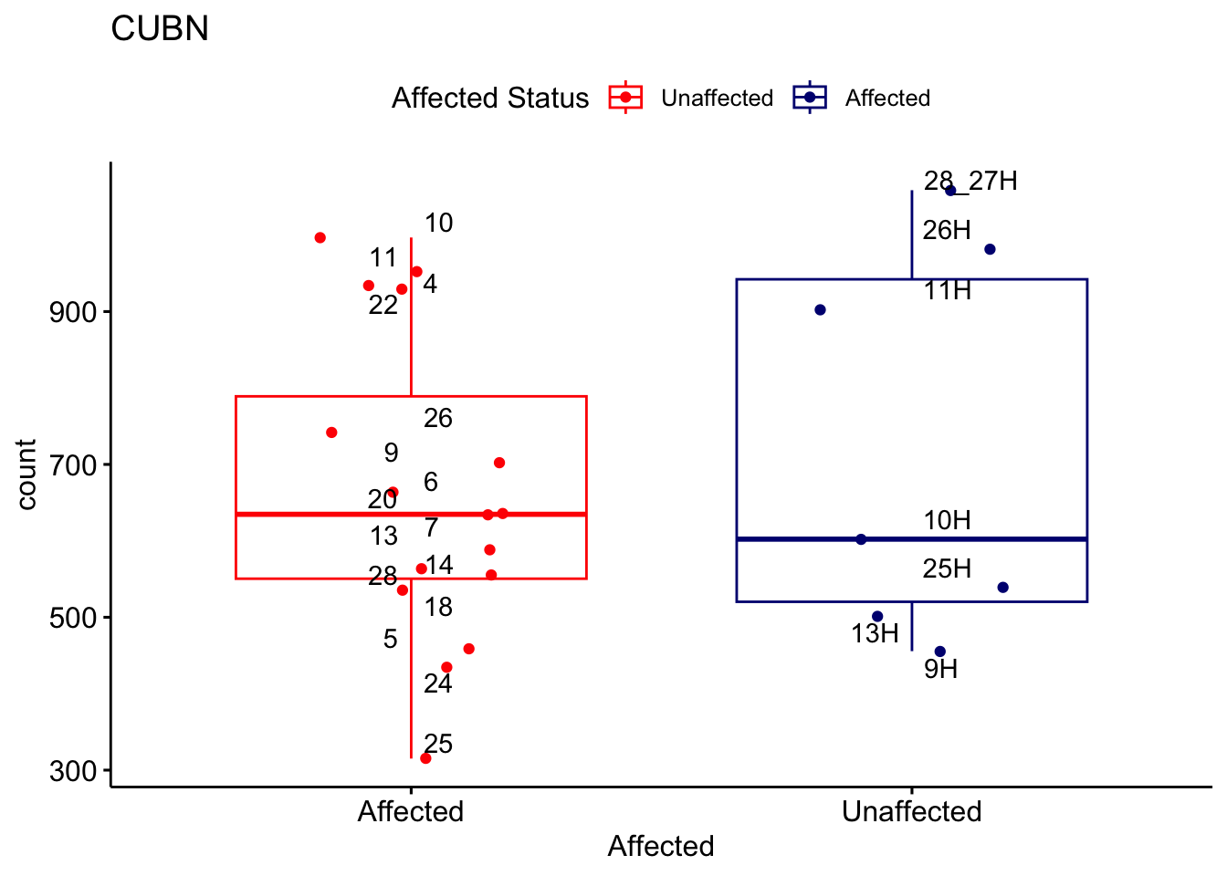
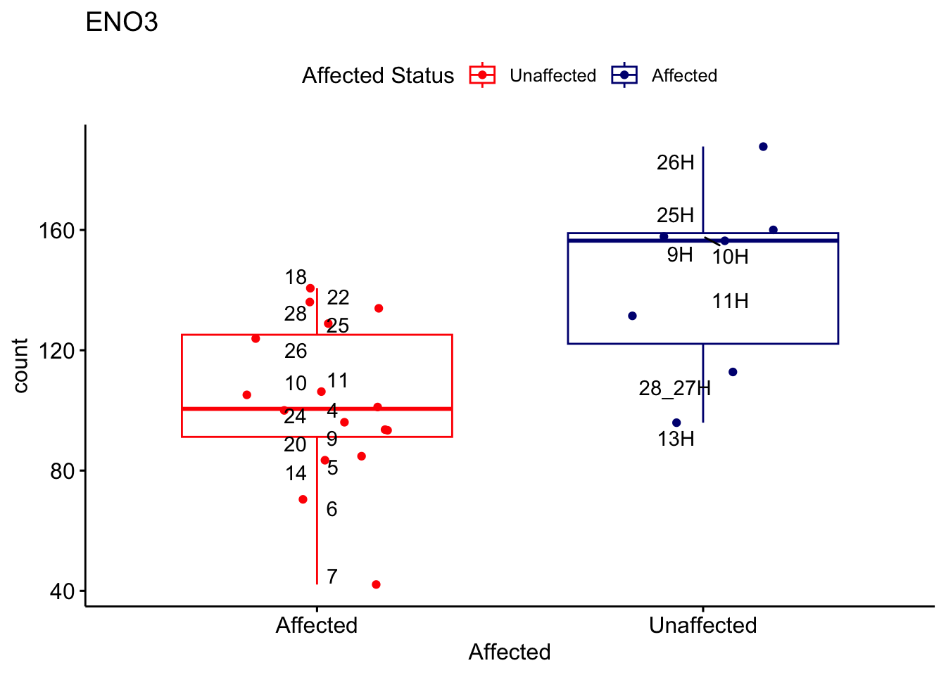
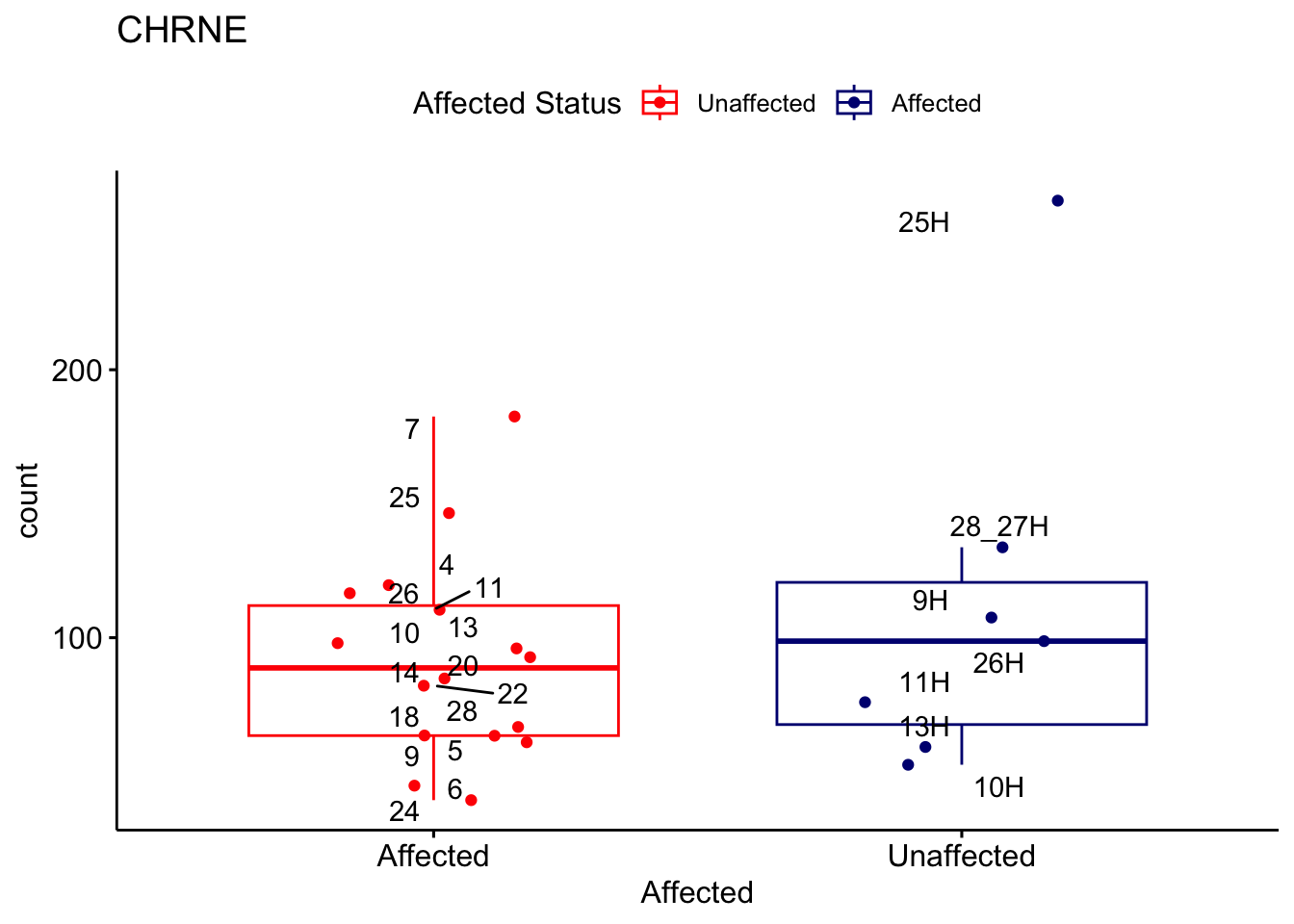
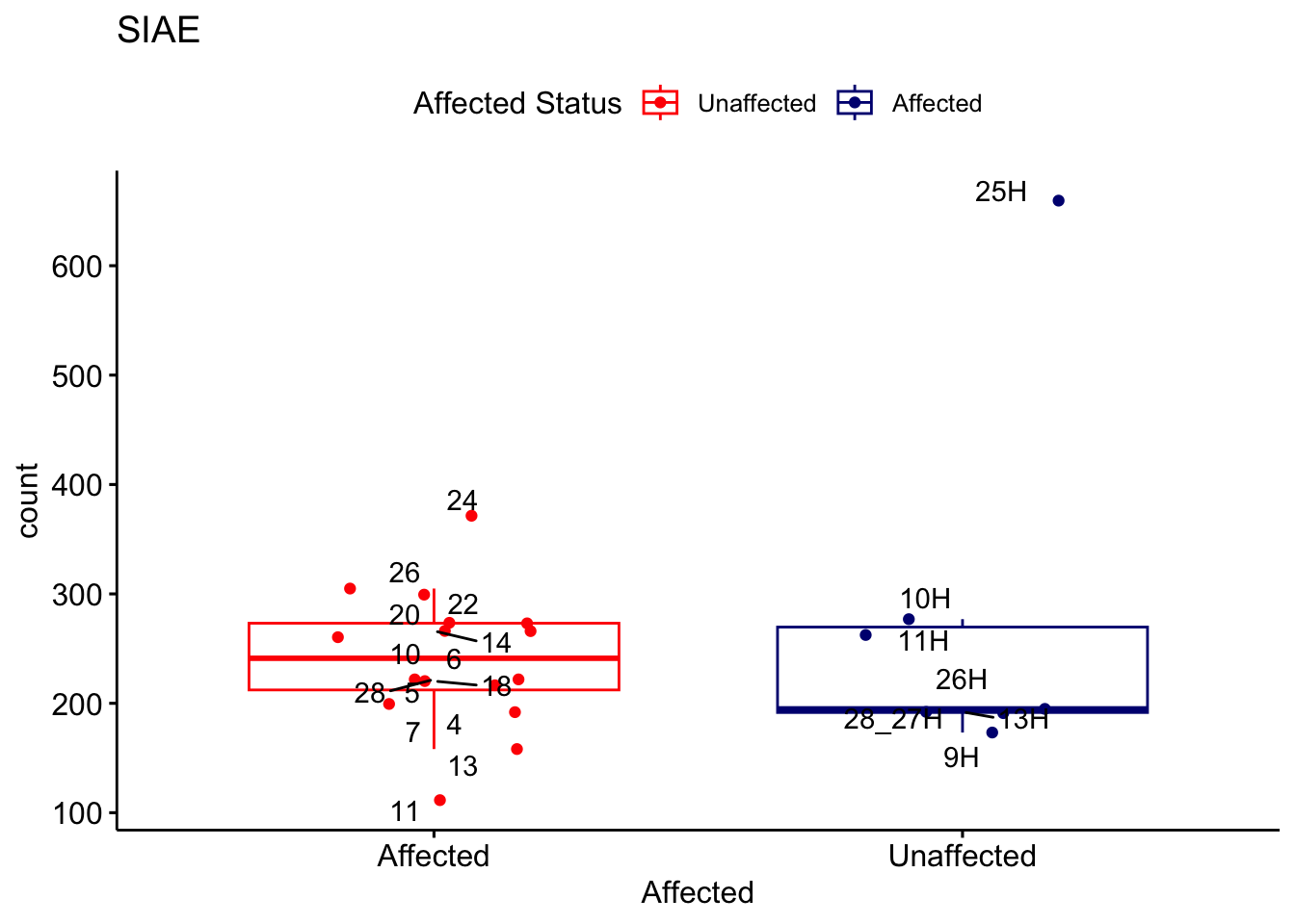
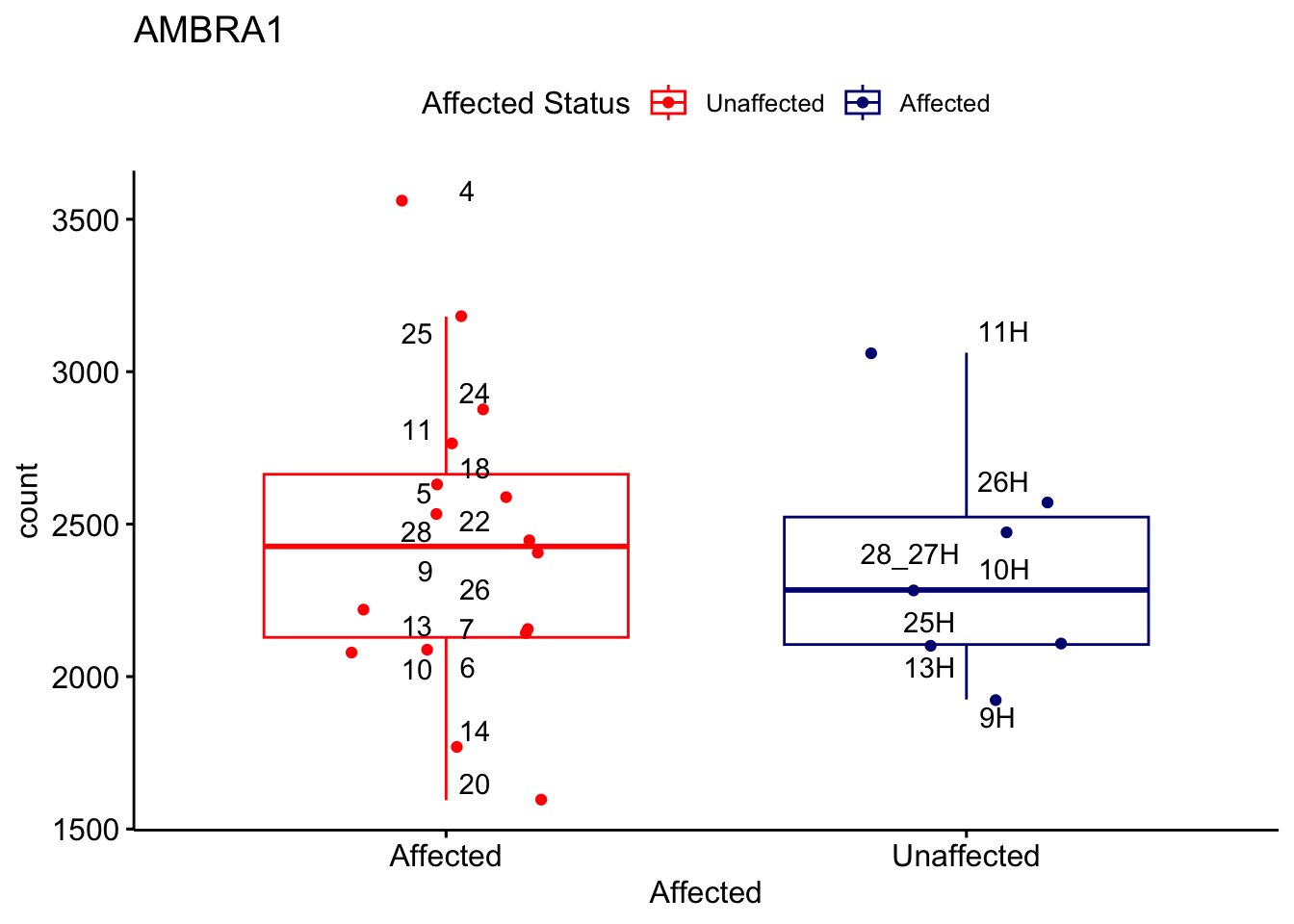
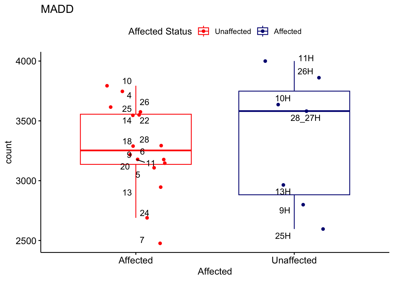
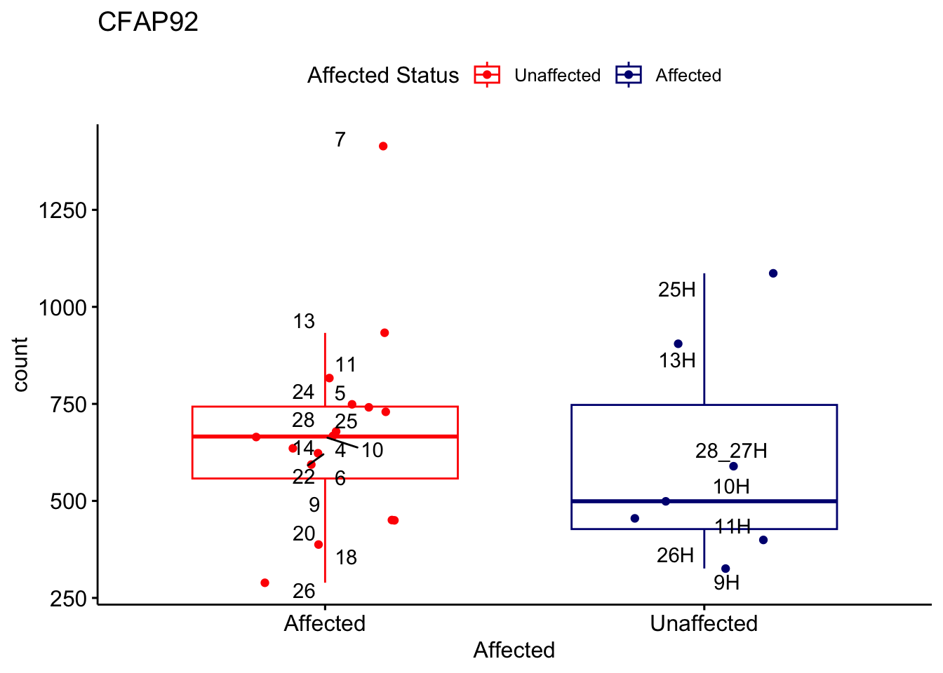
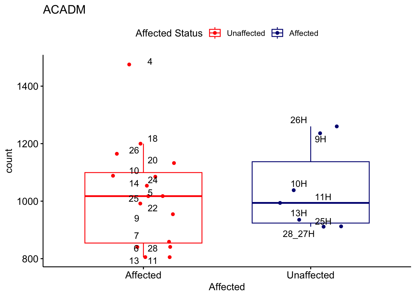
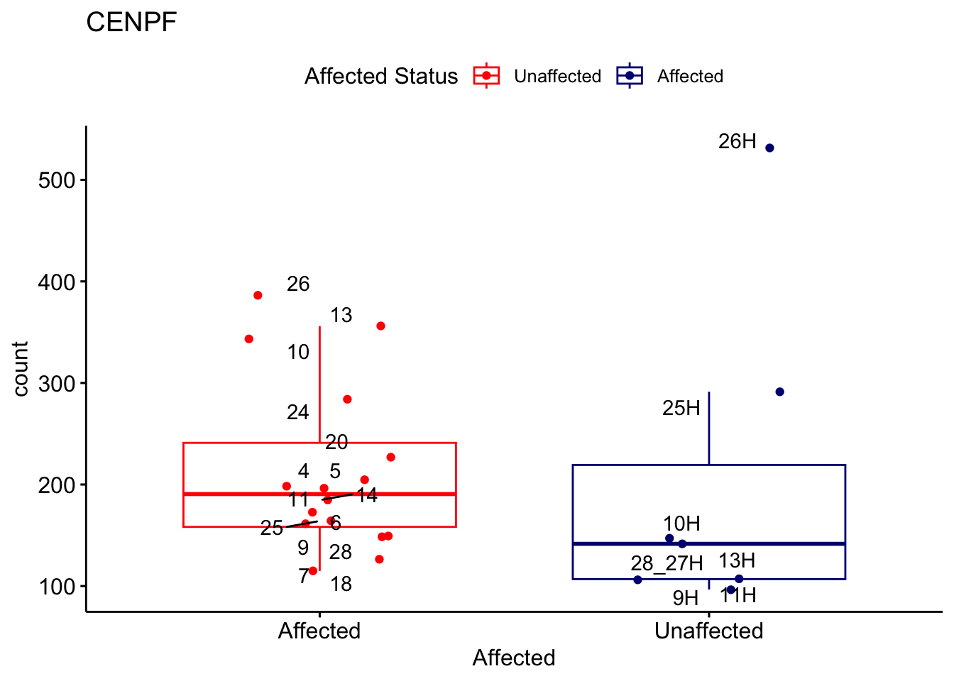
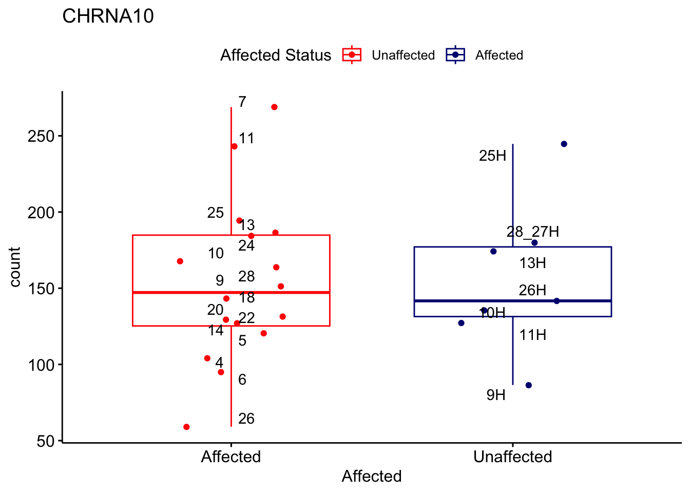
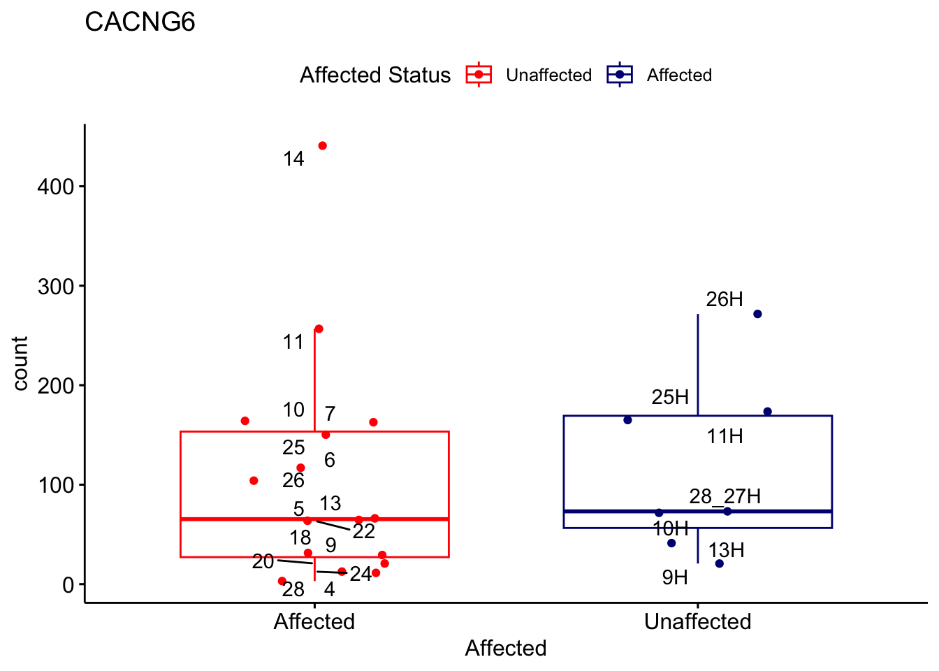
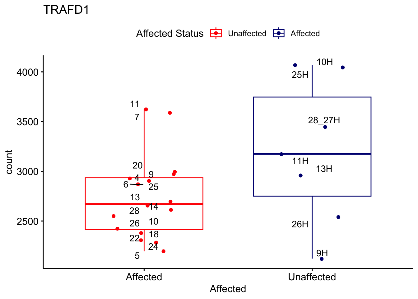
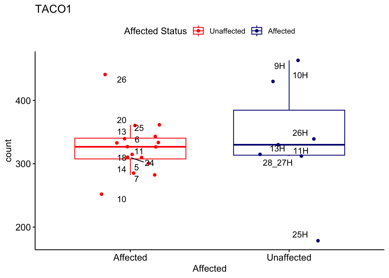
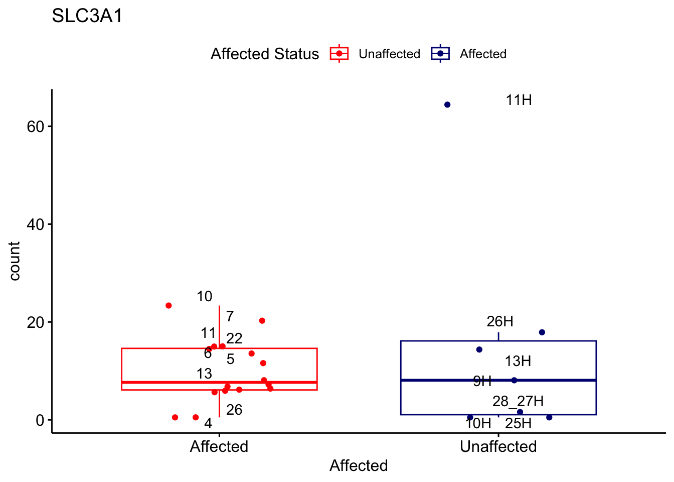
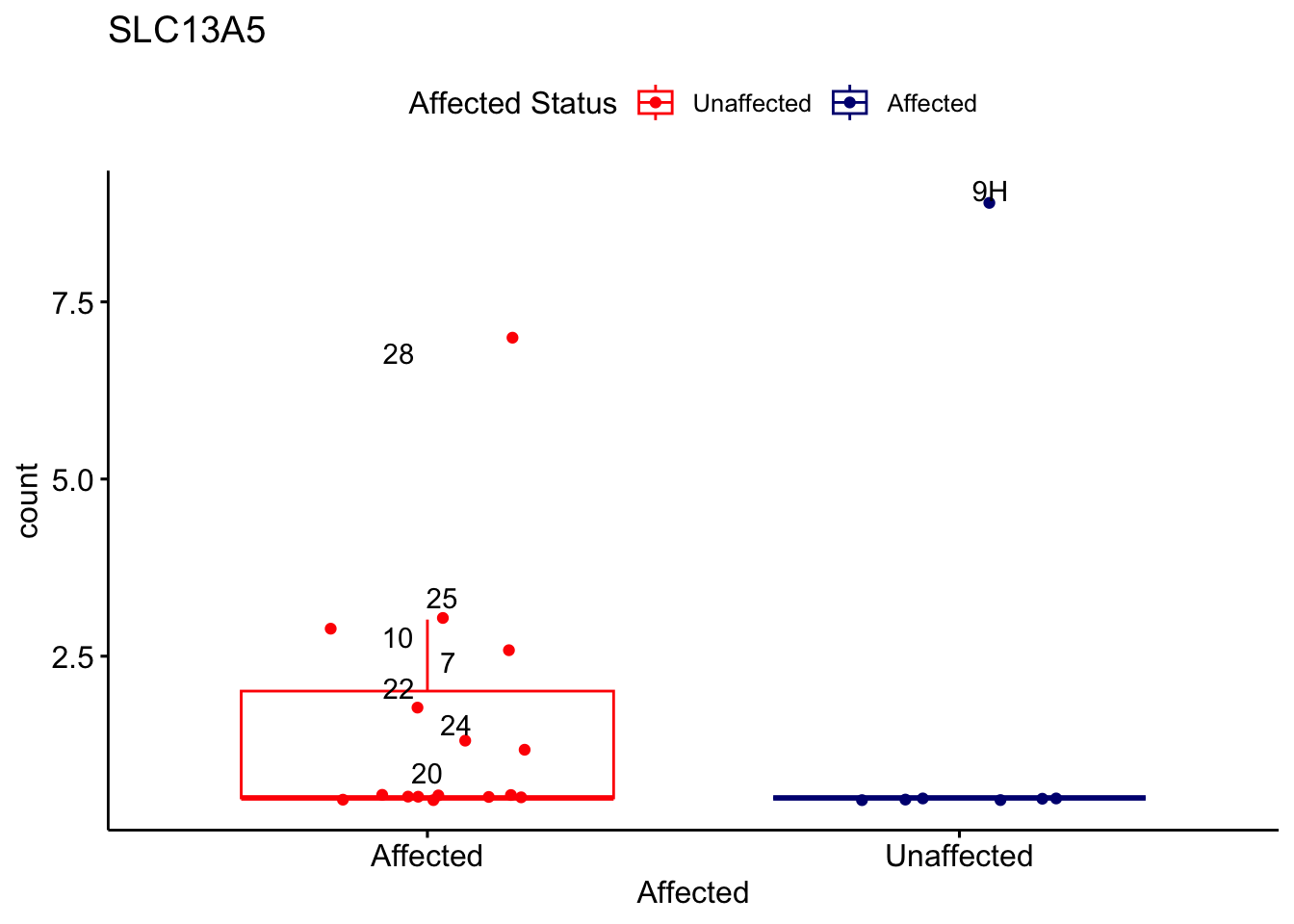
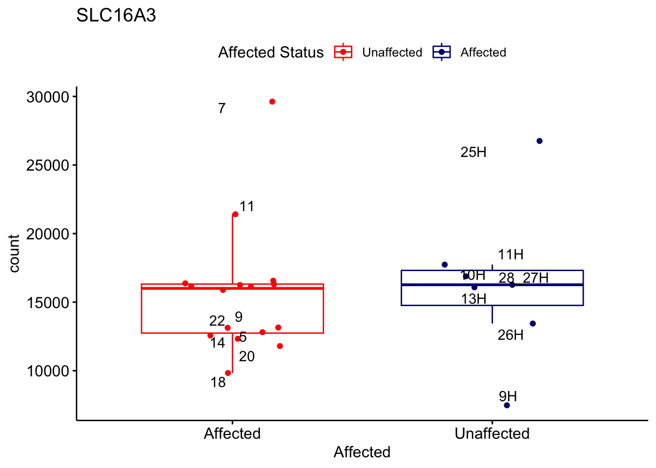
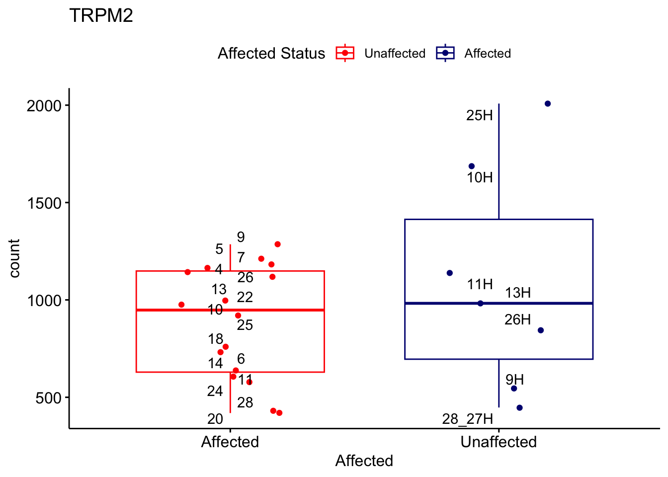
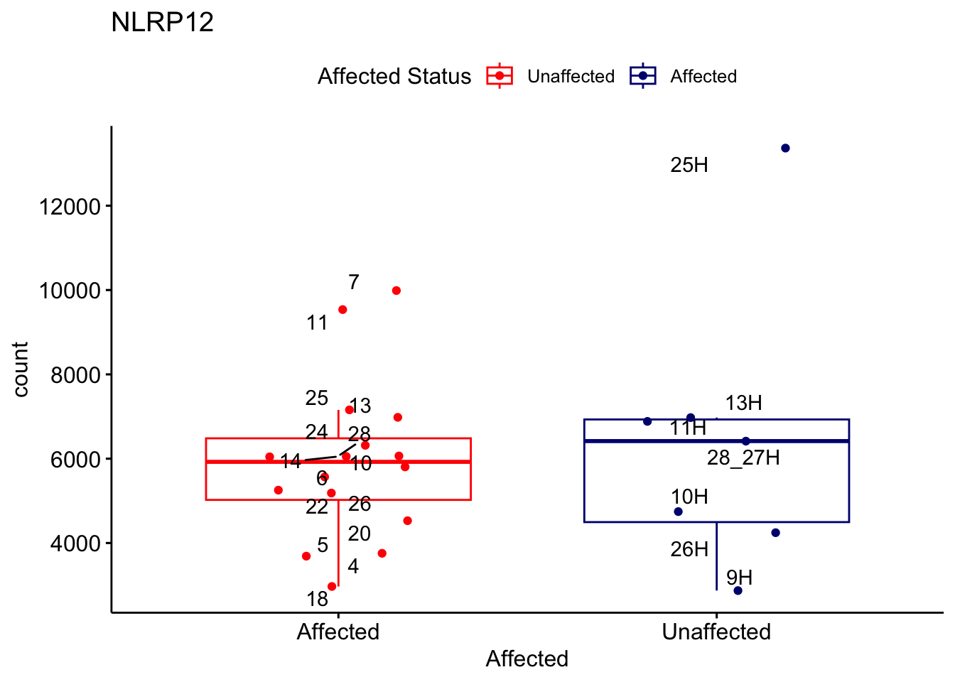
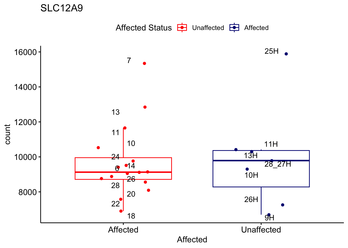
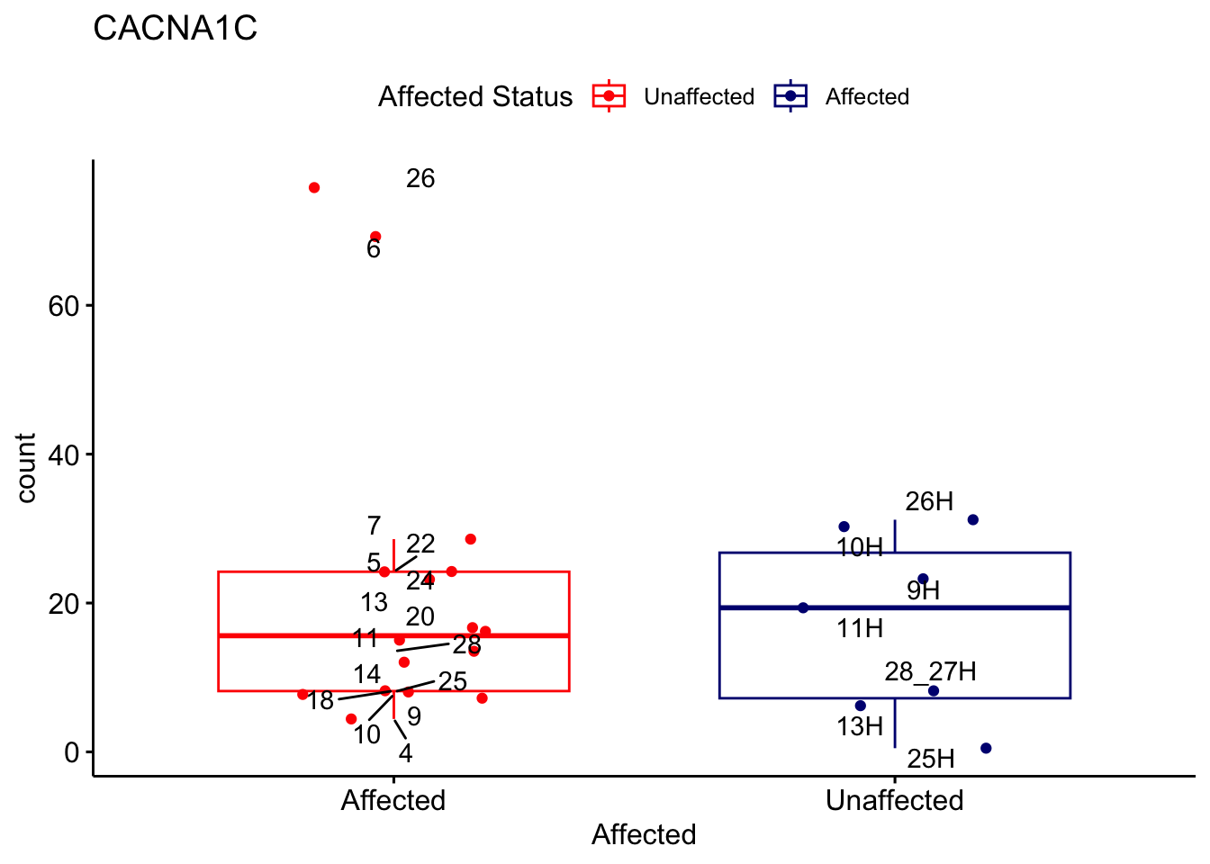
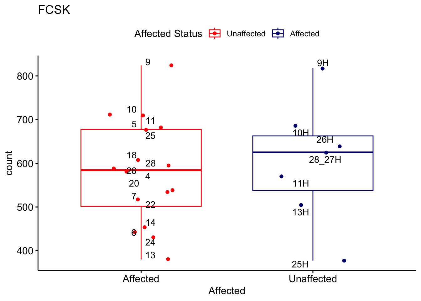
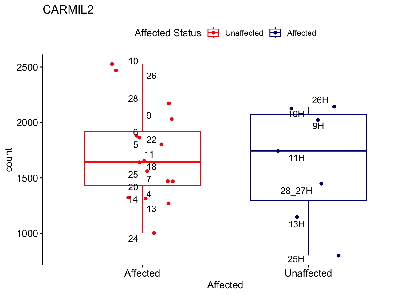
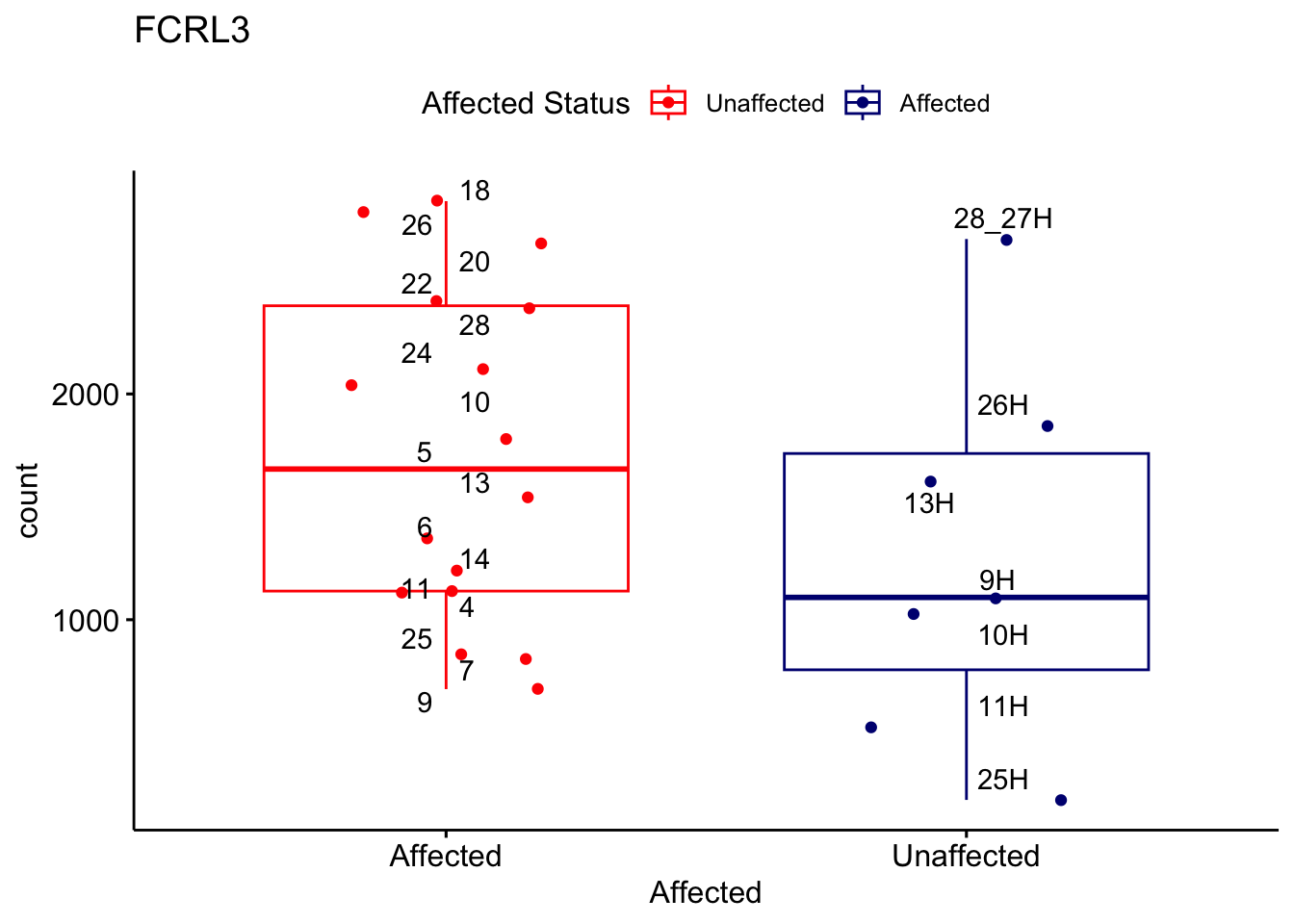
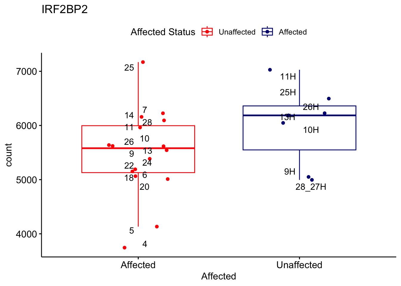
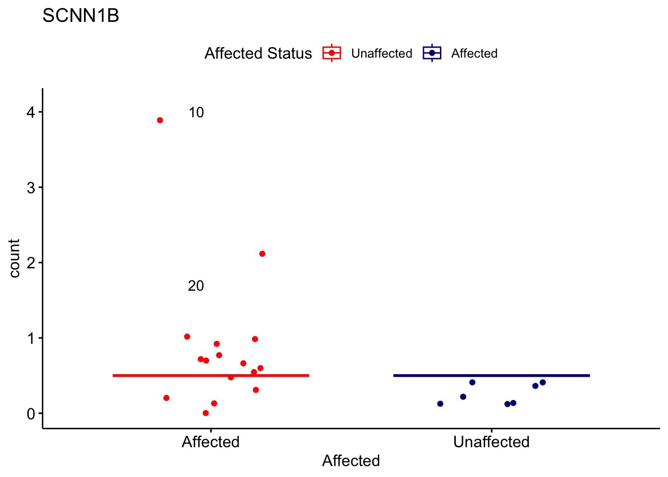
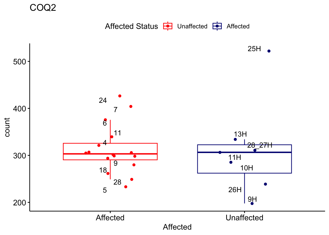
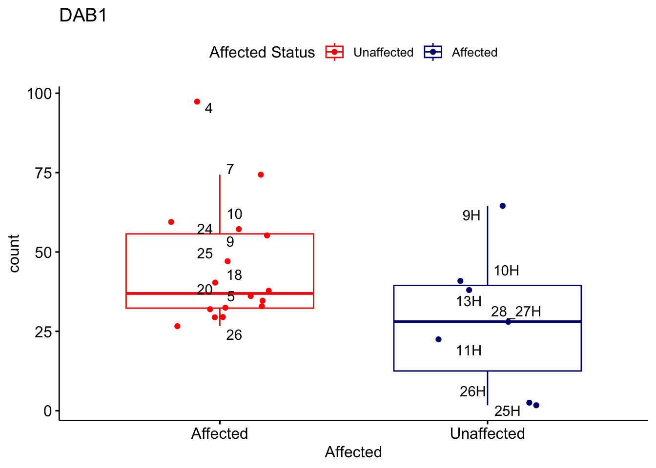
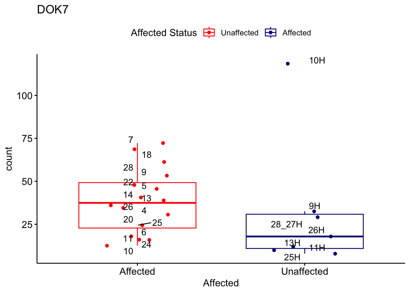
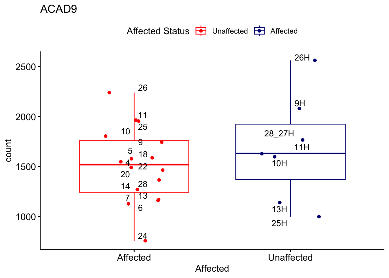
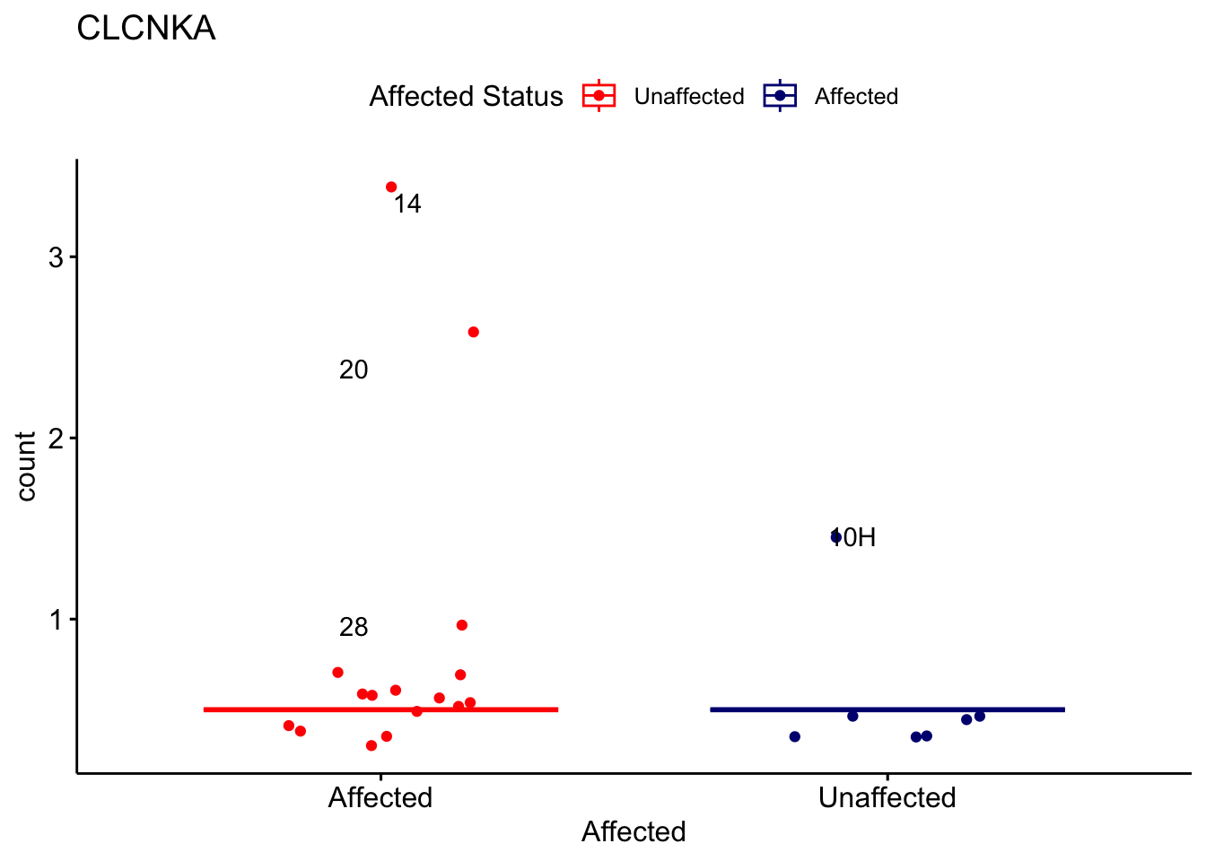
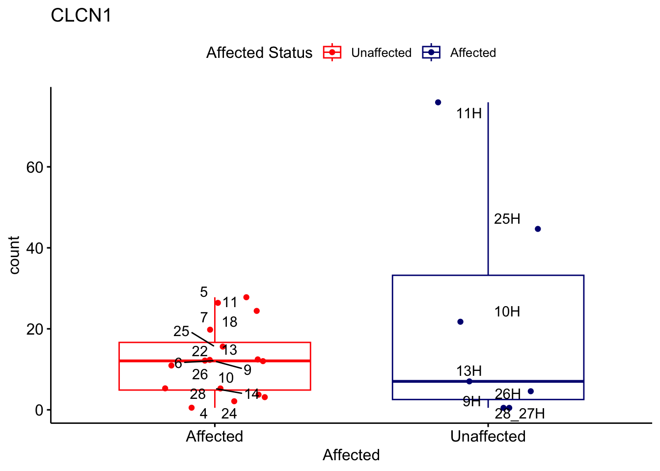
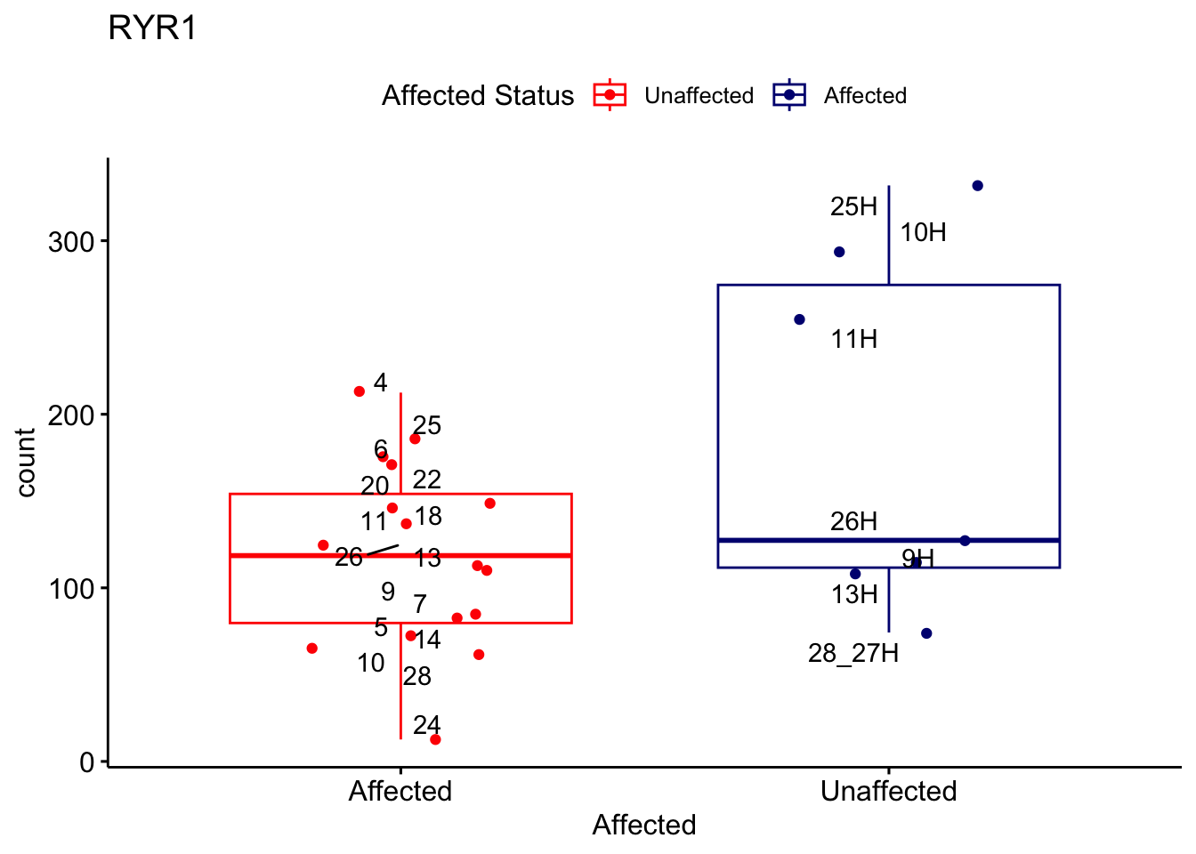
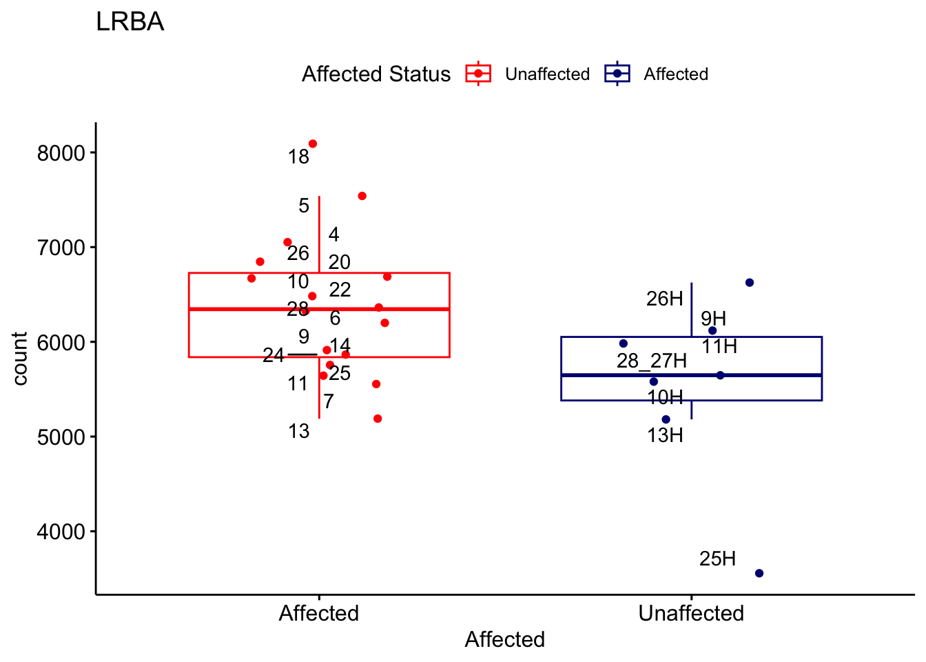
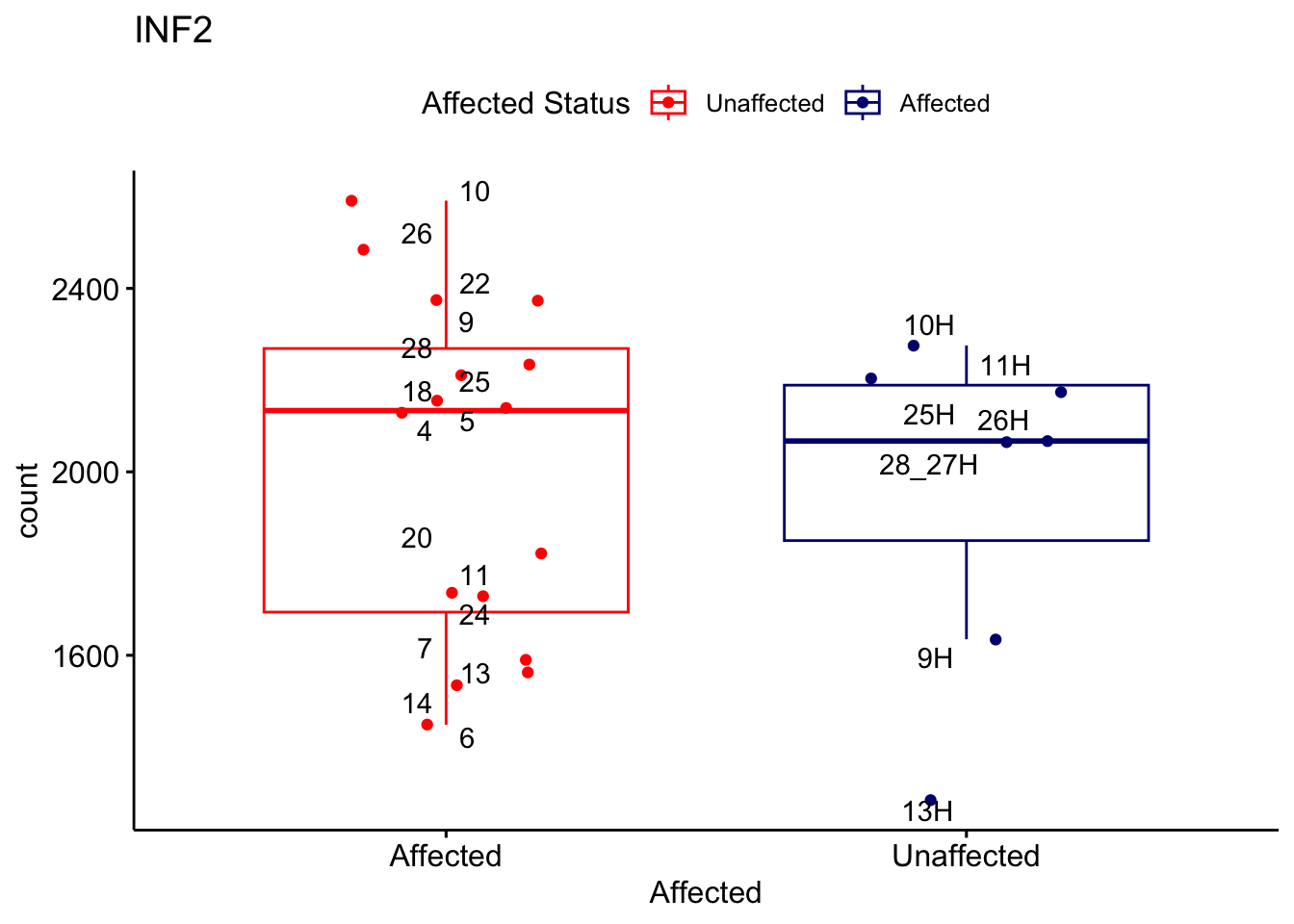
library(STRINGdb)Plot Counts
# For loop for plot counts
for (ensembl_id in filtered_by_interest$Ensembl_ID) {
  d <- plotCounts(dds, gene = ensembl_id, intgroup = "Affected", returnData = TRUE)
  gene_name <- filtered_by_interest$gene_name[filtered_by_interest$Ensembl_ID == ensembl_id]
  ggplot_box <- ggboxplot(d, x = "Affected", y = "count", add = "jitter",
                          color = "Affected", palette = c("red", "navy"),
                          title = gene_name) +
    geom_text_repel(aes(label = rownames(d))) +
    scale_color_manual(name = "Affected Status",
                       labels = c("Unaffected", "Affected"),
                       values = c("red", "navy"))
  print(ggplot_box) # Ensure each plot is printed during the loop
  ggsave(
    filename = paste0(gene_name, "-subsetted-plot-counts.png"),
    path = "output/batch-correction-limma/plot-counts",
    plot = ggplot_box, dpi = 450
  )
}
Save data
save.image(file = "output/subsetted-condition-analysis.RData")
sessionInfo()R version 4.3.2 (2023-10-31)
Platform: x86_64-apple-darwin20 (64-bit)
Running under: macOS Sonoma 14.4
Matrix products: default
BLAS: /Library/Frameworks/R.framework/Versions/4.3-x86_64/Resources/lib/libRblas.0.dylib
LAPACK: /Library/Frameworks/R.framework/Versions/4.3-x86_64/Resources/lib/libRlapack.dylib; LAPACK version 3.11.0
locale:
[1] en_US.UTF-8/en_US.UTF-8/en_US.UTF-8/C/en_US.UTF-8/en_US.UTF-8
time zone: America/Chicago
tzcode source: internal
attached base packages:
[1] stats4 stats graphics grDevices utils datasets methods
[8] base
other attached packages:
[1] STRINGdb_2.12.1 mygene_1.36.0
[3] GenomicFeatures_1.52.2 ReactomePA_1.44.0
[5] ggrepel_0.9.5 UpSetR_1.4.0
[7] org.Hs.eg.db_3.17.0 AnnotationDbi_1.62.2
[9] DOSE_3.26.2 clusterProfiler_4.8.3
[11] ggupset_0.3.0.9002 rmarkdown_2.26
[13] ggpubr_0.6.0 plotly_4.10.4
[15] biomaRt_2.56.1 gprofiler2_0.2.3
[17] limma_3.56.2 genefilter_1.82.1
[19] pheatmap_1.0.12 RColorBrewer_1.1-3
[21] DESeq2_1.40.2 SummarizedExperiment_1.30.2
[23] Biobase_2.60.0 MatrixGenerics_1.12.3
[25] matrixStats_1.2.0 GenomicRanges_1.52.1
[27] GenomeInfoDb_1.36.4 IRanges_2.34.1
[29] S4Vectors_0.38.2 BiocGenerics_0.46.0
[31] lubridate_1.9.3 forcats_1.0.0
[33] stringr_1.5.1 dplyr_1.1.4
[35] purrr_1.0.2 readr_2.1.5
[37] tidyr_1.3.1 tibble_3.2.1
[39] ggplot2_3.5.0 tidyverse_2.0.0
[41] workflowr_1.7.1
loaded via a namespace (and not attached):
[1] fs_1.6.3 bitops_1.0-7 enrichplot_1.20.3
[4] HDO.db_0.99.1 httr_1.4.7 doParallel_1.0.17
[7] tools_4.3.2 backports_1.4.1 utf8_1.2.4
[10] R6_2.5.1 lazyeval_0.2.2 GetoptLong_1.0.5
[13] withr_3.0.0 graphite_1.46.0 prettyunits_1.2.0
[16] gridExtra_2.3 textshaping_0.3.7 cli_3.6.2
[19] scatterpie_0.2.1 labeling_0.4.3 sass_0.4.8
[22] systemfonts_1.0.6 Rsamtools_2.16.0 yulab.utils_0.1.4
[25] foreign_0.8-86 gson_0.1.0 plotrix_3.8-4
[28] rstudioapi_0.15.0 RSQLite_2.3.5 BiocIO_1.10.0
[31] generics_0.1.3 gridGraphics_0.5-1 shape_1.4.6.1
[34] gtools_3.9.5 vroom_1.6.5 car_3.1-2
[37] GO.db_3.17.0 Matrix_1.6-5 fansi_1.0.6
[40] abind_1.4-5 lifecycle_1.0.4 whisker_0.4.1
[43] yaml_2.3.8 carData_3.0-5 gplots_3.1.3.1
[46] qvalue_2.32.0 BiocFileCache_2.11.1 grid_4.3.2
[49] blob_1.2.4 promises_1.2.1 crayon_1.5.2
[52] lattice_0.22-5 cowplot_1.1.3 annotate_1.78.0
[55] KEGGREST_1.40.1 magick_2.8.3 pillar_1.9.0
[58] knitr_1.45 ComplexHeatmap_2.16.0 fgsea_1.26.0
[61] rjson_0.2.21 codetools_0.2-19 fastmatch_1.1-4
[64] glue_1.7.0 getPass_0.2-4 downloader_0.4
[67] ggfun_0.1.4 data.table_1.15.2 vctrs_0.6.5
[70] png_0.1-8 treeio_1.24.3 gtable_0.3.4
[73] gsubfn_0.7 cachem_1.0.8 xfun_0.42
[76] S4Arrays_1.0.6 tidygraph_1.3.1 survival_3.5-8
[79] iterators_1.0.14 nlme_3.1-164 ggtree_3.8.2
[82] bit64_4.0.5 progress_1.2.3 filelock_1.0.3
[85] rprojroot_2.0.4 bslib_0.6.1 KernSmooth_2.23-22
[88] rpart_4.1.23 Hmisc_5.1-2 colorspace_2.1-0
[91] DBI_1.2.2 nnet_7.3-19 tidyselect_1.2.1
[94] processx_3.8.3 chron_2.3-61 bit_4.0.5
[97] compiler_4.3.2 curl_5.2.1 git2r_0.33.0
[100] graph_1.78.0 htmlTable_2.4.2 xml2_1.3.6
[103] DelayedArray_0.26.7 rtracklayer_1.60.1 shadowtext_0.1.3
[106] caTools_1.18.2 checkmate_2.3.1 scales_1.3.0
[109] callr_3.7.5 rappdirs_0.3.3 digest_0.6.35
[112] XVector_0.40.0 base64enc_0.1-3 htmltools_0.5.7
[115] pkgconfig_2.0.3 highr_0.10 dbplyr_2.4.0
[118] fastmap_1.1.1 rlang_1.1.3 GlobalOptions_0.1.2
[121] htmlwidgets_1.6.4 ggthemes_5.1.0 farver_2.1.1
[124] jquerylib_0.1.4 jsonlite_1.8.8 BiocParallel_1.34.2
[127] GOSemSim_2.26.1 RCurl_1.98-1.14 magrittr_2.0.3
[130] Formula_1.2-5 GenomeInfoDbData_1.2.10 ggplotify_0.1.2
[133] patchwork_1.2.0 munsell_0.5.0 Rcpp_1.0.12
[136] proto_1.0.0 ape_5.7-1 viridis_0.6.5
[139] sqldf_0.4-11 stringi_1.8.3 ggraph_2.2.1
[142] zlibbioc_1.46.0 MASS_7.3-60.0.1 plyr_1.8.9
[145] parallel_4.3.2 Biostrings_2.68.1 graphlayouts_1.1.1
[148] splines_4.3.2 hash_2.2.6.3 hms_1.1.3
[151] circlize_0.4.16 locfit_1.5-9.9 ps_1.7.6
[154] igraph_2.0.3 ggsignif_0.6.4 reshape2_1.4.4
[157] XML_3.99-0.16.1 evaluate_0.23 tzdb_0.4.0
[160] foreach_1.5.2 tweenr_2.0.3 httpuv_1.6.14
[163] polyclip_1.10-6 clue_0.3-65 ggforce_0.4.2
[166] broom_1.0.5 xtable_1.8-4 restfulr_0.0.15
[169] reactome.db_1.84.0 tidytree_0.4.6 rstatix_0.7.2
[172] later_1.3.2 ragg_1.3.0 viridisLite_0.4.2
[175] aplot_0.2.2 GenomicAlignments_1.36.0 memoise_2.0.1
[178] cluster_2.1.6 timechange_0.3.0