classification
wiesehahn
2020-07-28
Last updated: 2020-08-19
Checks: 6 1
Knit directory: baumarten/analysis/
This reproducible R Markdown analysis was created with workflowr (version 1.6.2). The Checks tab describes the reproducibility checks that were applied when the results were created. The Past versions tab lists the development history.
The R Markdown file has unstaged changes. To know which version of the R Markdown file created these results, you’ll want to first commit it to the Git repo. If you’re still working on the analysis, you can ignore this warning. When you’re finished, you can run wflow_publish to commit the R Markdown file and build the HTML.
Great job! The global environment was empty. Objects defined in the global environment can affect the analysis in your R Markdown file in unknown ways. For reproduciblity it’s best to always run the code in an empty environment.
The command set.seed(20200723) was run prior to running the code in the R Markdown file. Setting a seed ensures that any results that rely on randomness, e.g. subsampling or permutations, are reproducible.
Great job! Recording the operating system, R version, and package versions is critical for reproducibility.
Nice! There were no cached chunks for this analysis, so you can be confident that you successfully produced the results during this run.
Great job! Using relative paths to the files within your workflowr project makes it easier to run your code on other machines.
Great! You are using Git for version control. Tracking code development and connecting the code version to the results is critical for reproducibility.
The results in this page were generated with repository version 83c54a6. See the Past versions tab to see a history of the changes made to the R Markdown and HTML files.
Note that you need to be careful to ensure that all relevant files for the analysis have been committed to Git prior to generating the results (you can use wflow_publish or wflow_git_commit). workflowr only checks the R Markdown file, but you know if there are other scripts or data files that it depends on. Below is the status of the Git repository when the results were generated:
Ignored files:
    Ignored:    .Rhistory
    Ignored:    .Rproj.user/
    Ignored:    analysis/.Rhistory
    Ignored:    data/sen2/

Untracked files:
    Untracked:  data/models/
    Untracked:  data/reference/train_test/

Unstaged changes:
    Modified:   analysis/classification.Rmd
Note that any generated files, e.g. HTML, png, CSS, etc., are not included in this status report because it is ok for generated content to have uncommitted changes.
These are the previous versions of the repository in which changes were made to the R Markdown (analysis/classification.Rmd) and HTML (docs/classification.html) files. If you’ve configured a remote Git repository (see ?wflow_git_remote), click on the hyperlinks in the table below to view the files as they were in that past version.
| File | Version | Author | Date | Message |
|---|---|---|---|---|
| Rmd | 9e1da18 | wiesehahn | 2020-08-11 | update |
Classification
Model Tuning
A number of model parameters can be changed to achieve different results. Model tuning changes these parameters to get optimal results. Overfitting might be a problem. Parameters to be changed in all classifiers are input variables (bands and indices in our case) and training data.
Hyperparameters in the random forest package include:
ntree (Integer, default: 500): Number of trees to grow.
mtry (Integer, Defaults to the square root of the number of variables) The number of variables per split.
nodesize (Integer, default: 1): The minimum size of a terminal node.
Gridsearch Results
The number of trees was held constant at a value of 500 because generally it is assumed that more trees give better performance. On the other side larger numbers also mean more processing time. Parameters for which a gridsearch was done are the number of variables per split and the minimum terminal node size.
Random Forest

21346 samples
   26 predictor
    6 classes: 'BU', 'DGL', 'FI', 'KI', 'LAE', 'TEI'

No pre-processing
Resampling: Cross-Validated (10 fold)
Summary of sample sizes: 19213, 19210, 19211, 19212, 19213, 19212, ...
Resampling results across tuning parameters:

  mtry  min.node.size  Accuracy   Kappa
  2      1             0.9125360  0.8871864
  2      5             0.9121145  0.8866175
  2     10             0.9107092  0.8847945
  3      1             0.9135673  0.8885034
  3      5             0.9146911  0.8899728
  3     10             0.9130044  0.8877618
  4      1             0.9153943  0.8908709
  4      5             0.9149721  0.8903133
  4     10             0.9139884  0.8890256
  6      1             0.9173147  0.8933482
  6      5             0.9170336  0.8929783
  6     10             0.9154409  0.8909142
  8      1             0.9178770  0.8940709
  8      5             0.9175957  0.8937008
  8     10             0.9163312  0.8920810

Tuning parameter 'splitrule' was held constant at a value of gini
Accuracy was used to select the optimal model using the largest value.
The final values used for the model were mtry = 8, splitrule = gini
 and min.node.size = 1.
plotted gridsearch result for the number of predictor variables and minimal node size
As we can see the differences are not very pronounced. Hence, a simpler model results in similar performance. Based on these results we can simplify our model in terms of minimal node size and variables per split without deteriorating the results.
Model Simplification
Here we search for the simplest model without deteriorating the performance (max 2% difference to best model).
| mtry | splitrule | min.node.size | Accuracy | Kappa | AccuracySD | KappaSD |
|---|---|---|---|---|---|---|
| 2 | gini | 1 | 0.912536 | 0.8871864 | 0.0072623 | 0.0094074 |
The results indicate that in terms of prediction accuracy a model with least variables per split (2) and a minimal node size of 1 is sufficient enough.
Model Validation
To have a closer look at the model performance the validation data is classified with the best model obtained by gridsearch.
Error Matrix| Baumart | BU | DGL | FI | KI | LAE | TEI |
|---|---|---|---|---|---|---|
| BU | 2244 | 1 | 3 | 1 | 69 | 124 |
| DGL | 4 | 423 | 59 | 20 | 4 | 1 |
| FI | 0 | 62 | 2728 | 18 | 2 | 0 |
| KI | 2 | 20 | 37 | 484 | 31 | 0 |
| LAE | 94 | 17 | 16 | 43 | 824 | 45 |
| TEI | 63 | 5 | 5 | 2 | 39 | 1654 |
| Accuracy | Kappa | AccuracyLower | AccuracyUpper |
|---|---|---|---|
| 0.9139326 | 0.8891244 | 0.9079967 | 0.9196033 |
Variable Importance
As determined before, model parameters minimal node size and variables per split have limited influence on model performance. As a consequence it is likely that the choice of predictor variables is important for model performance.
Input variables considered as predictor variables in this study comprise:
Sentinel-2 bands and indices - Bands: ‘B2’,‘B3’,‘B4’,‘B5’,‘B6’,‘B7’,‘B8’,‘B8A’,‘B11’,‘B12’ ??? - Indices: ???
In model fitting the relative variable importance is calculated to give an impression which predictor variables are valuable and which are less valuable for the prediction process. However, correlation between variables is not taken into account.
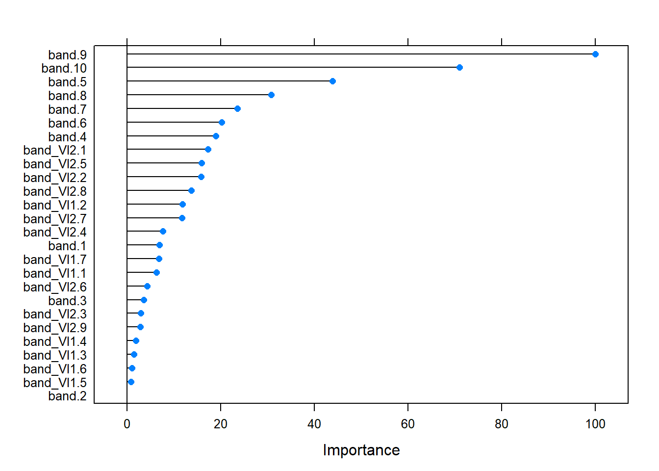
Relative predictor variable importance
As we can see the importance metric varies between predictor variables, suggesting that the choice of predictor variables very much influences our model. While more predictor variables might add information they are also complicating the model and might even introduce noise. Hence, a reduction of predictor variables might enhance our model.
Feature Selection
To further simplify the prediction model a Recursive Feature Elimitaion (rfe) is applied. This will eliminate worst performing predictor variables (chosen by importance) at each step and keep the best performing variables to end up in a reduced number of predictor variables which perform best in model prediction.
Number of Features
model performance by number of features evaluated with Recursive Feature Elimitaion
The best model in regards to predictor variables uses 16 out of 26 variables. However, we can see that the model performs equally good with less predictor variables.
Chosen variables
| prediction features | |
|---|---|
| 1 | band.9 |
| 2 | band.10 |
| 3 | band_VI2.8 |
| 4 | band_VI1.2 |
| 5 | band_VI2.7 |
| 6 | band_VI2.2 |
| 7 | band_VI1.7 |
| 8 | band_VI2.5 |
| 9 | band_VI2.4 |
| 10 | band.1 |
| 11 | band.5 |
| 12 | band.8 |
| 13 | band_VI1.1 |
| 14 | band_VI2.9 |
| 15 | band_VI2.1 |
| 16 | band_VI2.6 |
Model Simplification
To simplify the model without loosing prediction accuracy we search for a model with less predictor variables, which has the same accuracy as the best performing model (max 2 % difference in accuracy).
As a result we get a model using the following 6 prediction variables instead of all 26 variables, which has almost the same accuracy.
Chosen variables
| prediction features | |
|---|---|
| 1 | band.9 |
| 2 | band.10 |
| 3 | band_VI2.8 |
| 4 | band_VI1.2 |
| 5 | band_VI2.7 |
| 6 | band_VI2.2 |
Respective Accuracy
| Variables | Accuracy | Kappa | AccuracySD | KappaSD |
|---|---|---|---|---|
| 6 | 0.9035971 | 0.8756644 | 0.005679 | 0.0073154 |
Final Model
Using the results from previous analysis we train a model with best performing predictor variables and model-hyperparameters.
The predictor variables are listed in @ref(tab:rfe_tab_predictors_simp):
The hyperparameters are:
- Number of variables to possibly split at in each node (mtry) = 2
- Minimal node size = 1
- Number of trees = 500 (this was not optimized, as more trees usually give better results but the maximum number is limited by computation power)
Model Validation
Applying the final model to predict tree species for the validation data set, the error matrix looks like this:
| Baumart | BU | DGL | FI | KI | LAE | TEI |
|---|---|---|---|---|---|---|
| BU | 2219 | 1 | 3 | 0 | 103 | 130 |
| DGL | 2 | 402 | 70 | 24 | 4 | 1 |
| FI | 0 | 82 | 2716 | 21 | 9 | 0 |
| KI | 5 | 27 | 40 | 458 | 42 | 1 |
| LAE | 99 | 14 | 18 | 65 | 790 | 29 |
| TEI | 82 | 2 | 1 | 0 | 21 | 1663 |
Respective Accuracy
| Accuracy | Kappa | AccuracyLower | AccuracyUpper |
|---|---|---|---|
| 0.9020122 | 0.8736537 | 0.8957353 | 0.9080317 |
Model using Sentinel-2 bands
| Accuracy | Kappa | AccuracyLower | AccuracyUpper |
|---|---|---|---|
| 0.9108705 | 0.8851401 | 0.904844 | 0.9166337 |
Model using Sentinel-2 indices
| Accuracy | Kappa | AccuracyLower | AccuracyUpper |
|---|---|---|---|
| 0.9011374 | 0.8721306 | 0.8948365 | 0.9071813 |
Model using Sentinel-2 bands and indices
| Accuracy | Kappa | AccuracyLower | AccuracyUpper |
|---|---|---|---|
| 0.9139326 | 0.8891162 | 0.9079967 | 0.9196033 |
Model probability
R version 4.0.2 (2020-06-22)
Platform: i386-w64-mingw32/i386 (32-bit)
Running under: Windows 10 x64 (build 18362)

Matrix products: default

locale:
[1] LC_COLLATE=German_Germany.1252  LC_CTYPE=German_Germany.1252
[3] LC_MONETARY=German_Germany.1252 LC_NUMERIC=C
[5] LC_TIME=German_Germany.1252

attached base packages:
[1] stats     graphics  grDevices utils     datasets  methods   base

other attached packages:
 [1] forcats_0.5.0     stringr_1.4.0     purrr_0.3.4       tidyr_1.1.0
 [5] tibble_3.0.3      tidyverse_1.3.0   ranger_0.12.1     caret_6.0-86
 [9] lattice_0.20-41   recipes_0.1.13    dplyr_1.0.0       here_0.1
[13] plotly_4.9.2.1    ggplot2_3.3.2     readr_1.3.1       kableExtra_1.1.0
[17] viridis_0.5.1     viridisLite_0.3.0

loaded via a namespace (and not attached):
 [1] nlme_3.1-148         fs_1.4.2             lubridate_1.7.9
 [4] RColorBrewer_1.1-2   webshot_0.5.2        httr_1.4.2
 [7] rprojroot_1.3-2      tools_4.0.2          backports_1.1.7
[10] R6_2.4.1             rpart_4.1-15         DBI_1.1.0
[13] lazyeval_0.2.2       colorspace_1.4-1     nnet_7.3-14
[16] withr_2.2.0          tidyselect_1.1.0     gridExtra_2.3
[19] compiler_4.0.2       git2r_0.27.1         cli_2.0.2
[22] rvest_0.3.6          xml2_1.3.2           scales_1.1.1
[25] digest_0.6.25        rmarkdown_2.3        pkgconfig_2.0.3
[28] htmltools_0.5.0      highr_0.8            dbplyr_1.4.4
[31] readxl_1.3.1         htmlwidgets_1.5.1    rlang_0.4.7
[34] rstudioapi_0.11      farver_2.0.3         generics_0.0.2
[37] jsonlite_1.7.0       crosstalk_1.1.0.1    ModelMetrics_1.2.2.2
[40] magrittr_1.5         Matrix_1.2-18        fansi_0.4.1
[43] Rcpp_1.0.5           munsell_0.5.0        lifecycle_0.2.0
[46] stringi_1.4.6        whisker_0.4          pROC_1.16.2
[49] yaml_2.2.1           MASS_7.3-51.6        plyr_1.8.6
[52] grid_4.0.2           blob_1.2.1           promises_1.1.1
[55] crayon_1.3.4         haven_2.3.1          splines_4.0.2
[58] hms_0.5.3            knitr_1.29           pillar_1.4.6
[61] reshape2_1.4.4       codetools_0.2-16     stats4_4.0.2
[64] reprex_0.3.0         glue_1.4.1           evaluate_0.14
[67] data.table_1.12.8    modelr_0.1.8         vctrs_0.3.2
[70] httpuv_1.5.4         foreach_1.5.0        cellranger_1.1.0
[73] gtable_0.3.0         assertthat_0.2.1     xfun_0.15
[76] gower_0.2.2          prodlim_2019.11.13   broom_0.7.0
[79] e1071_1.7-3          later_1.1.0.1        class_7.3-17
[82] survival_3.2-3       timeDate_3043.102    iterators_1.0.12
[85] workflowr_1.6.2      lava_1.6.7           ellipsis_0.3.1
[88] ipred_0.9-9