Comparing initialization functions (part II)
Jason Willwerscheid
8/28/2018
Last updated: 2018-08-29
workflowr checks: (Click a bullet for more information)-
✔ R Markdown file: up-to-date
Great! Since the R Markdown file has been committed to the Git repository, you know the exact version of the code that produced these results.
-
✔ Environment: empty
Great job! The global environment was empty. Objects defined in the global environment can affect the analysis in your R Markdown file in unknown ways. For reproduciblity it’s best to always run the code in an empty environment.
-
✔ Seed:
set.seed(20180714)The command
set.seed(20180714)was run prior to running the code in the R Markdown file. Setting a seed ensures that any results that rely on randomness, e.g. subsampling or permutations, are reproducible. -
✔ Session information: recorded
Great job! Recording the operating system, R version, and package versions is critical for reproducibility.
-
Great! You are using Git for version control. Tracking code development and connecting the code version to the results is critical for reproducibility. The version displayed above was the version of the Git repository at the time these results were generated.✔ Repository version: 237072b
Note that you need to be careful to ensure that all relevant files for the analysis have been committed to Git prior to generating the results (you can usewflow_publishorwflow_git_commit). workflowr only checks the R Markdown file, but you know if there are other scripts or data files that it depends on. Below is the status of the Git repository when the results were generated:
Note that any generated files, e.g. HTML, png, CSS, etc., are not included in this status report because it is ok for generated content to have uncommitted changes.Ignored files: Ignored: .DS_Store Ignored: .Rhistory Ignored: .Rproj.user/ Ignored: docs/.DS_Store Ignored: docs/figure/.DS_Store Untracked files: Untracked: code/init_fn3.R Untracked: data/greedy19.rds Untracked: data/init_fn3/
Expand here to see past versions:
| File | Version | Author | Date | Message |
|---|---|---|---|---|
| Rmd | 237072b | Jason Willwerscheid | 2018-08-29 | wflow_publish(“analysis/init_fn3.Rmd”) |
Introduction
Here I return to the question of which initialization function is best, and in which cases. I run some simple experiments on simulated datasets of various dimensions and with or without missing data.
Results
I simulate data from both a null model and a rank-one model with \(p \in \{1000, 10000\}\) and with \(n\) ranging from 10 to 1000. I either retain all of the data or I delete 20% of entries. I initialize using "udv_si", "udv_si_svd", and, when there is no missing data, "udv_svd".
I pre-run the code below and load the results from file.
all_res <- readRDS("./data/init_fn3/all_res.rds")

plot_results <- function(res, n, main, colors) {
  colors = colors[c("udv_si_svd", "udv_si", "udv_svd")]
  plot(log10(n), log10(res[["udv_si_svd"]]), type='l', col=colors[1],
       xlab = "log10(n)", ylab = "time elapsed (log10 s)",
       ylim = log10(c(min(unlist(res)), max(unlist(res)))),
       main = main)
  lines(log10(n), log10(res[["udv_si"]]), col=colors[2])
  if (length(res) == 3) {
    lines(log10(n), log10(res[["udv_svd"]]), col=colors[3])
  }

  legend.txt <- c("udv_si_svd", "udv_si", "udv_svd")
  legend("bottomright", legend.txt[1:length(res)], lty=1,
         col=colors[1:length(res)])
}

ns <- c(10, 25, 50, 100, 250, 500, 1000)
colors = RColorBrewer::brewer.pal(3, "Dark2")[1:3]
names(colors) = c("udv_svd", "udv_si", "udv_si_svd")

plot_results(all_res$null_noNA_p1000, ns,
             "Null data (no missing), p = 1000", colors)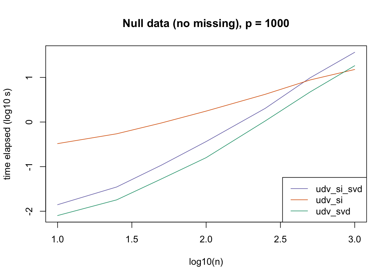
plot_results(all_res$null_noNA_p10000, ns,
             "Null data (no missing), p = 10000", colors)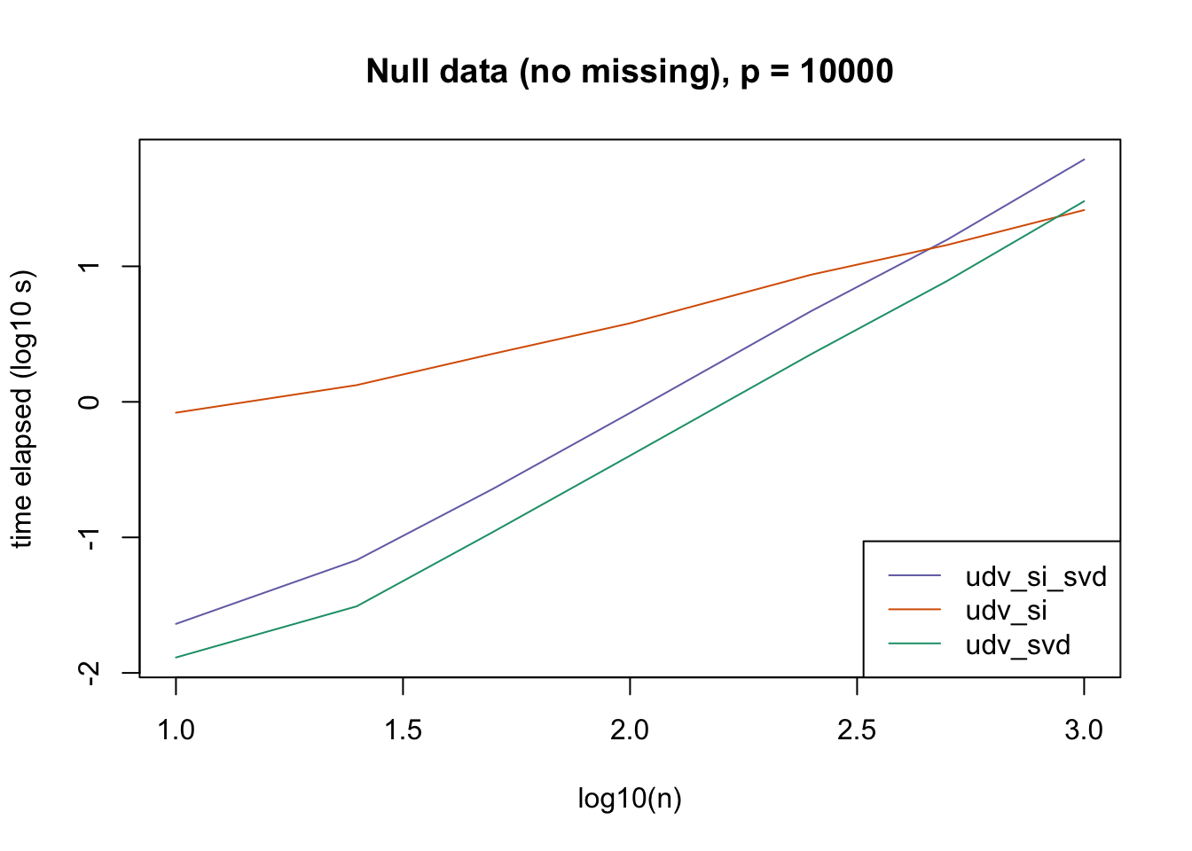
plot_results(all_res$r1_noNA_p1000, ns,
             "Rank-one data (no missing), p = 1000", colors)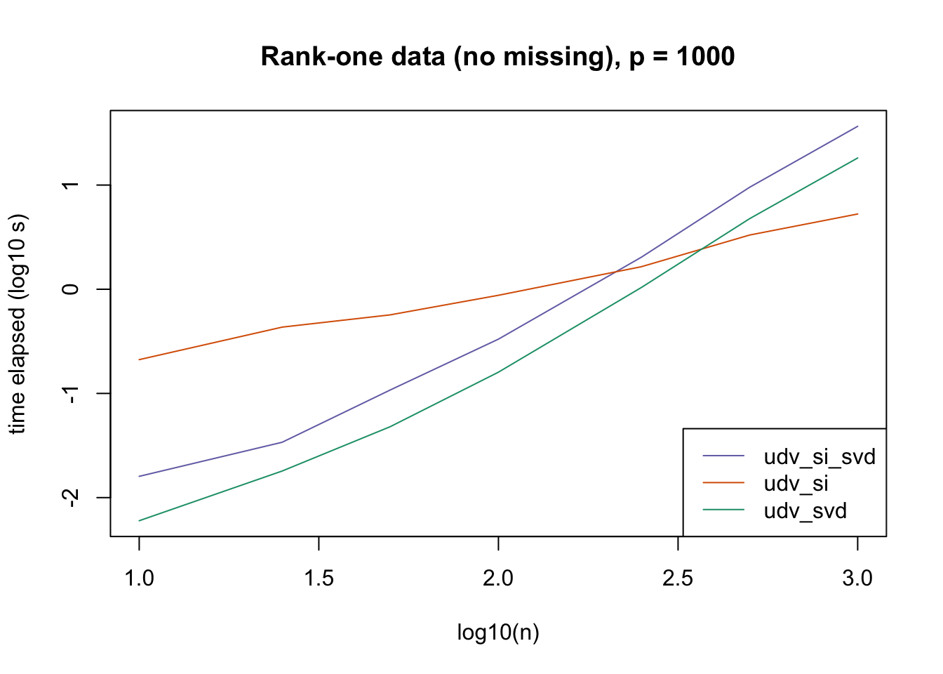
plot_results(all_res$r1_noNA_p10000, ns,
             "Rank-one data (no missing), p = 10000", colors)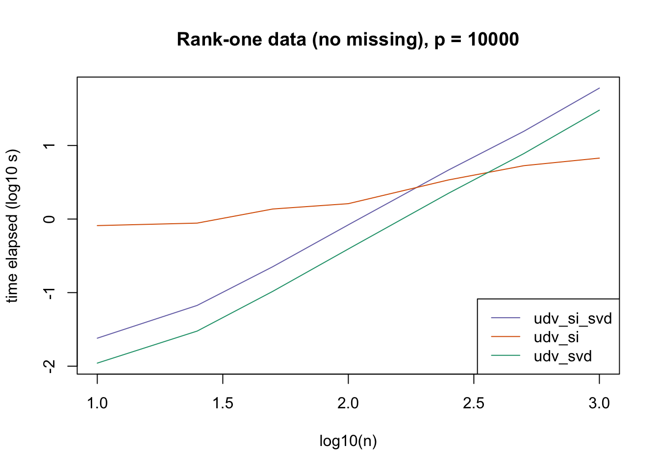
plot_results(all_res$null_missing_p1000, ns,
             "Null data (with missing), p = 1000", colors)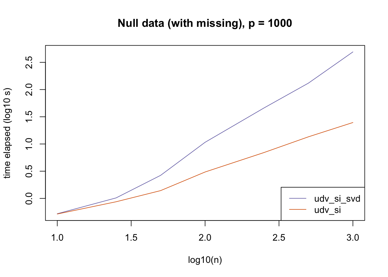
plot_results(all_res$null_missing_p10000, ns,
             "Null data (with missing), p = 10000", colors)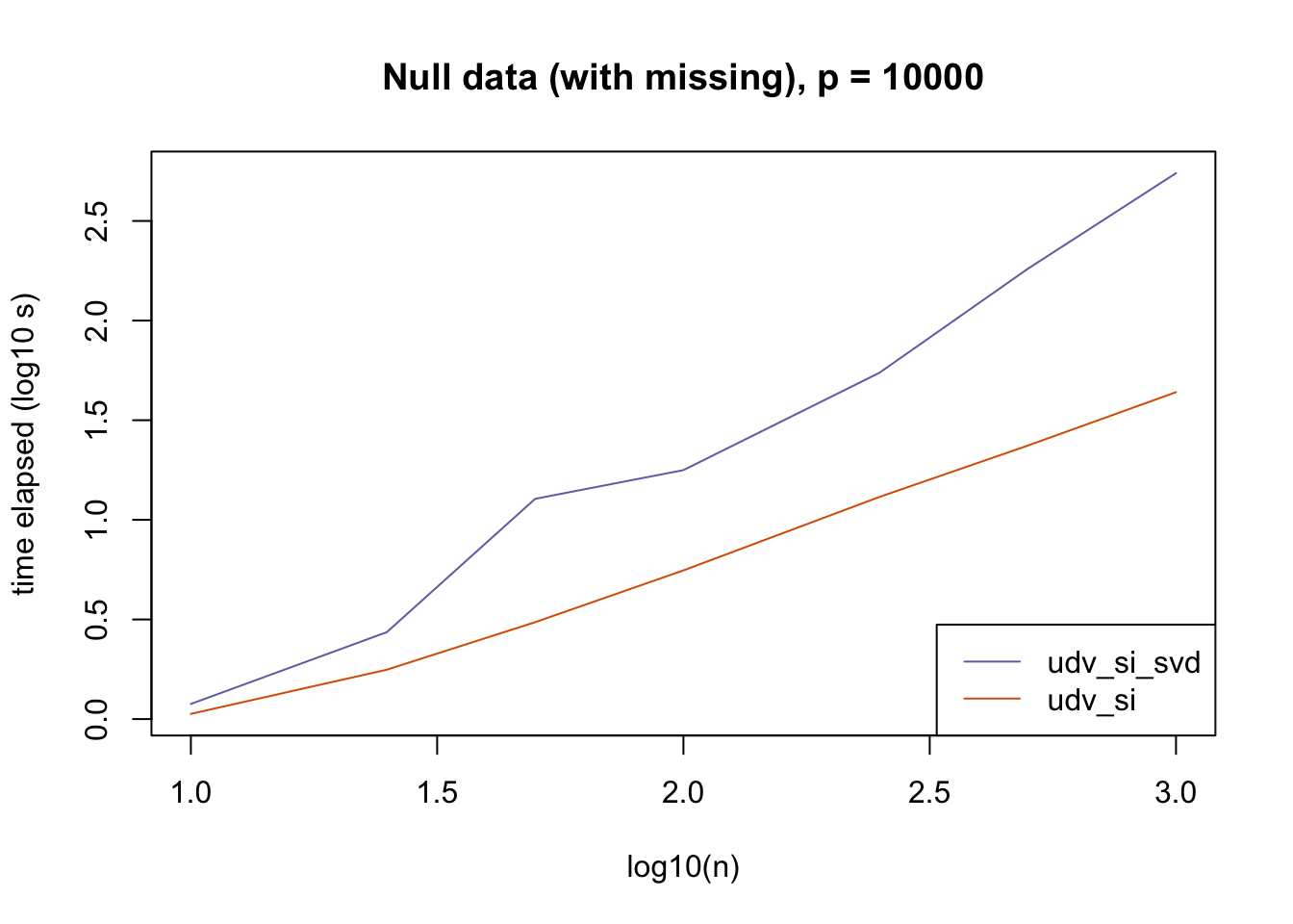
plot_results(all_res$r1_missing_p1000, ns,
             "Rank-one data (with missing), p = 1000", colors)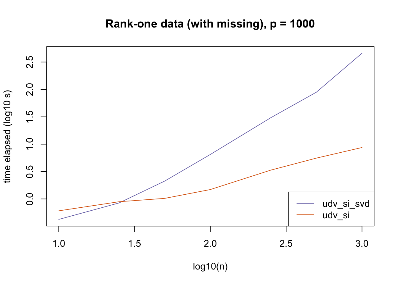
plot_results(all_res$r1_missing_p10000, ns,
             "Rank-one data (with missing), p = 10000", colors)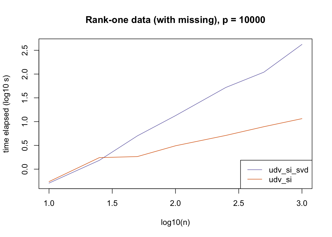
Conclusions
The current default init_fn = "udv_si" is sensible. In cases with missing data, "udv_si" almost always beats "udv_si_svd"; the only exceptions are for small \(n\), but in such cases initialization is very fast anyway.
When there is no missing data, then "udv_svd" is the fastest method for small \(n\), but "udv_si" is again the fastest method when \(n\) becomes large. (Interestingly, the relative speeds do not seem to depend on the larger dimension \(p\).)
It would be possible to programmatically set init_fn based on \(n\) (or more precisely, based on the smaller of \(n\) and \(p\)), but I don’t think it’s worth the trouble, since "udv_si_svd" seems to consistently be the fastest (or nearly fastest) method when the speed of initialization actually becomes an issue.
Code
devtools::load_all("/Users/willwerscheid/GitHub/flashr")

sim_mat <- function(n, p, type, missing) {
  if (type == 1) {
    out <- matrix(rnorm(n * p), nrow=n, ncol=p)
  } else if (type == 2) {
    out <- (outer(rep(1, n), rep(1, p))
            + matrix(rnorm(n * p), nrow=n, ncol=p))
  }
  if (missing) {
    out[rbinom(n * p, 1, 0.2) == 1] <- NA
  }
  return(out)
}

do_experiment <- function(nreps, ns, p, type, missing, verbose=TRUE) {
  res <- list()
  if (missing) {
    init_fns <- c("udv_si", "udv_si_svd")
  } else {
    init_fns <- c("udv_svd", "udv_si", "udv_si_svd")
  }

  for (init_fn in init_fns) {
    res[[init_fn]] <- rep(NA, nrow=length(ns))
  }

  for (i in 1:length(ns)) {
    if (verbose) {
      message("n = ", ns[i])
    }

    data <- list()
    for (rep in 1:nreps) {
      data[[rep]] <- sim_mat(ns[i], p, type, missing)
    }

    for (init_fn in init_fns) {
      t <- system.time({
        for (rep in 1:nreps) {
          fl <- flash_add_factors_from_data(data[[rep]],
                                            K=5,
                                            init_fn=init_fn,
                                            backfit=FALSE,
                                            verbose=FALSE)
        }
      })
      res[[init_fn]][i] <- t["elapsed"]
    }

  }

  return(res)
}

set.seed(666)
all_res <- list()

nreps <- 5
ns <- c(10, 25, 50, 100, 250, 500, 1000)
p <- 1000

all_res$null_noNA_p1000 <- do_experiment(nreps, ns, p, type=1,
                                         missing=FALSE)
all_res$r1_noNA_p1000 <- do_experiment(nreps, ns, p, type=2,
                                       missing=FALSE)
all_res$null_missing_p1000 <- do_experiment(nreps, ns, p, type=1,
                                            missing=TRUE)
all_res$r1_missing_p1000 <- do_experiment(nreps, ns, p, type=2,
                                          missing=TRUE)

nreps <- 1
ns <- c(10, 25, 50, 100, 250, 500, 1000)
p <- 10000

all_res$null_noNA_p10000 <- do_experiment(nreps, ns, p, type=1,
                                          missing=FALSE)
all_res$r1_noNA_p10000 <- do_experiment(nreps, ns, p, type=2,
                                        missing=FALSE)
all_res$null_missing_p10000 <- do_experiment(nreps, ns, p, type=1,
                                             missing=TRUE)
all_res$r1_missing_p10000 <- do_experiment(nreps, ns, p, type=2,
                                           missing=TRUE)

saveRDS(all_res, "./data/init_fn3/all_res.rds")
Session information
sessionInfo()R version 3.4.3 (2017-11-30)
Platform: x86_64-apple-darwin15.6.0 (64-bit)
Running under: macOS High Sierra 10.13.6
Matrix products: default
BLAS: /Library/Frameworks/R.framework/Versions/3.4/Resources/lib/libRblas.0.dylib
LAPACK: /Library/Frameworks/R.framework/Versions/3.4/Resources/lib/libRlapack.dylib
locale:
[1] en_US.UTF-8/en_US.UTF-8/en_US.UTF-8/C/en_US.UTF-8/en_US.UTF-8
attached base packages:
[1] stats graphics grDevices utils datasets methods base
loaded via a namespace (and not attached):
[1] workflowr_1.0.1 Rcpp_0.12.17 digest_0.6.15
[4] rprojroot_1.3-2 R.methodsS3_1.7.1 backports_1.1.2
[7] git2r_0.21.0 magrittr_1.5 evaluate_0.10.1
[10] stringi_1.1.6 whisker_0.3-2 R.oo_1.21.0
[13] R.utils_2.6.0 rmarkdown_1.8 RColorBrewer_1.1-2
[16] tools_3.4.3 stringr_1.3.0 yaml_2.1.17
[19] compiler_3.4.3 htmltools_0.3.6 knitr_1.20 This reproducible R Markdown analysis was created with workflowr 1.0.1