Matrix factorization of binary data

Introduction

I repeat the previous analysis but here I treat the GTEx donation matrix as binary data. (This is probably more appropriate; it is much more natural to assume that each donor will contribute a given tissue with a particular probability than that each donor will generate samples of a given tissue such that the count of samples is distributed as a Poisson random variable.)

Model

Here the model is $$Y_{ij} \sim \text{Bernoulli}(p_{ij}),$$ with $$\log \left( \frac{p}{1 - p} \right) = LF'.$$ As in the previous analysis, one could also put $$\log \left( \frac{p}{1 - p} \right) = LF' + E,$$ with the “errors” $E_{ij}$ distributed i.i.d. $N(0, \sigma^2)$.

Setting $\eta = \log (p / (1 - p))$, one has that $$\begin{aligned} \ell(\eta) &= \sum_{i, j} - \log (1 + e^{\eta_{ij}}) + Y_{ij} \eta_{ij} \\ \ell'(\eta) &= \sum_{i, j} -\frac{e^{\eta_{ij}}}{1 + e^{\eta_{ij}}} + Y_{ij} = \sum_{i, j} Y_{ij} - p_{ij} \\ \ell''(\eta) &= \sum_{i, j} - \frac{e^{\eta_{ij}}}{(1 + e^{\eta_{ij}})^2} = \sum_{i, j} -p_{ij}(1 - p_{ij}) \end{aligned}$$

Using the same trick as before, one obtains pseudo-data $$X = \log \left( \frac{p^\star}{1 - p^\star} \right) + \frac{Y - p^\star}{p^\star(1 - p^\star)}$$ with standard errors $$S = \frac{1}{\sqrt{p^\star(1 - p^\star)}}$$

The objective can be calculated as the FLASH objective plus $$\sum_{i, j} Y_{ij} \log p^\star_{ij} + (1 - Y_{ij}) \log (1 - p^\star_{ij}) + \frac{1}{2}\log \left( \frac{2 \pi}{p^\star_{ij}(1 - p^\star_{ij})} \right) + \frac{(Y_{ij} - p^\star_{ij})^2}{2p^\star_{ij}(1 - p^\star_{ij})}.$$

Code

This is largely cut and pasted from the previous analysis.

devtools::load_all("~/GitHub/flashr")
#> Loading flashr
devtools::load_all("~/GitHub/ebnm")
#> Loading ebnm

raw <- read.csv("https://storage.googleapis.com/gtex_analysis_v6/annotations/GTEx_Data_V6_Annotations_SampleAttributesDS.txt",
                header=TRUE, sep='\t')

data <- raw[, c("SAMPID", "SMTSD")] # sample ID, tissue type
# Extract donor ID:
tmp <- strsplit(as.character(data$SAMPID), "-")
data$SAMPID <- as.factor(sapply(tmp, function(x) {x[[2]]})) 
names(data) <- c("DonorID", "TissueType")

data <- suppressMessages(reshape2::acast(data, TissueType ~ DonorID))

missing.tissues <- c(1, 8, 9, 20, 21, 24, 26, 27, 33, 36, 39)
data <- data[-missing.tissues, ]

# Drop columns with no samples:
data <- data[, colSums(data) > 0]

# Convert to binary data:
data[data > 0] <- 1

gtex.colors <- read.table("https://github.com/stephenslab/gtexresults/blob/master/data/GTExColors.txt?raw=TRUE",
                          sep = '\t', comment.char = '')
gtex.colors <- gtex.colors[-c(7, 8, 19, 20, 24, 25, 31, 34, 37), 2]
gtex.colors <- as.character(gtex.colors)

# Computing objective (ELBO) -------------------------------------------

calc_obj <- function(fl, the_data, p) {
  return(fl$objective + 
           sum(the_data * log(p) + (1 - the_data) * log(1 - p) + 
                 0.5 * (log(2 * pi / (p * (1 - p))) + 
                          (the_data - p)^2 / (p * (1 - p)))))
}

# Calculating pseudo-data ----------------------------------------------

calc_X <- function(the_data, p) {
  return(log(p / (1 - p)) + (the_data - p) / (p * (1 - p)))
}

calc_S <- function(the_data, p) {
  return(1 / sqrt(p * (1 - p)))
}

set_pseudodata <- function(the_data, p) {
  return(flash_set_data(calc_X(the_data, p), S = calc_S(the_data, p)))
}

# Setting FLASH parameters ---------------------------------------------

# Initialization function for nonnegative loadings 
#   (but arbitrary factors):
my_init_fn <- function(Y, K = 1) {
  ret = udv_svd(Y, K)
  sum_pos = sum(ret$u[ret$u > 0]^2)
  sum_neg = sum(ret$u[ret$u < 0]^2)
  if (sum_neg > sum_pos) {
    return(list(u = -ret$u, d = ret$d, v = -ret$v))
  } else
    return(ret)
}

get_init_fn <- function(nonnegative = FALSE) {
  if (nonnegative) {
    return("my_init_fn")
  } else {
    return("udv_svd")
  }
}

get_ebnm_fn <- function(nonnegative = FALSE) {
  if (nonnegative) {
    return(list(l = "ebnm_ash", f = "ebnm_pn"))
  } else {
    return(list(l = "ebnm_pn", f = "ebnm_pn"))
  }
}

get_ebnm_param <- function(nonnegative = FALSE) {
  if (nonnegative) {
    return(list(l = list(mixcompdist = "+uniform"),
                f = list(warmstart = TRUE)))
  } else {
    return(list(l = list(warmstart = TRUE),
                f = list(warmstart = TRUE)))
  }
}

# Initializing p and running FLASH -------------------------------------

stabilize_p <- function(p) {
  p[p < 1e-6] <- 1e-6
  p[p > 1 - 1e-6] <- 1 - 1e-6
  return(p)
}

init_p <- function(the_data, f_init) {
  if (is.null(f_init)) {
    return(matrix(colMeans(the_data),
                  nrow = nrow(the_data), ncol = ncol(the_data),
                  byrow = TRUE))
  } else {
    p <- 1 / (1 + exp(-f_init$fitted_values))
    return(stabilize_p(p))
  }
}

update_p <- function(fl, pseudodata, var_type) {
  if (var_type == "constant") {
    LF <- fl$fitted_values
    X <- pseudodata$Y
    S2 <- pseudodata$S^2
    s2 <- 1 / fl$fit$tau[1, 1] - S2[1,1]
    eta <- LF + ((1 / S2) / (1 / S2 + 1 / s2)) * (X - LF)
    p <- 1 / (1 + exp(-eta))
  } else { # var_type = "zero"
    p <- 1 / (1 + exp(-fl$fitted_values))
  }
  return(stabilize_p(p))
}

greedy_iter <- function(pseudodata, f_init, niter, 
                        nonnegative = FALSE, var_type = "zero") {
  suppressWarnings(
    flash_greedy_workhorse(pseudodata,
                           Kmax = 1,
                           f_init = f_init,
                           var_type = var_type,
                           ebnm_fn = get_ebnm_fn(nonnegative),
                           ebnm_param = get_ebnm_param(nonnegative),
                           init_fn = get_init_fn(nonnegative),
                           verbose_output = "",
                           nullcheck = FALSE,
                           maxiter = niter)
  )
}

backfit_iter <- function(pseudodata, f_init, kset, niter, 
                         nonnegative = FALSE, var_type = "zero") {
  suppressWarnings(
    flash_backfit_workhorse(pseudodata,
                            kset = kset,
                            f_init = f_init,
                            var_type = var_type,
                            ebnm_fn = get_ebnm_fn(nonnegative),
                            ebnm_param = get_ebnm_param(nonnegative),
                            verbose_output = "",
                            nullcheck = FALSE,
                            maxiter = niter)
  )
}

run_one_fit <- function(the_data, f_init, greedy, maxiter = 200,
                        n_subiter = 200, nonnegative = FALSE, 
                        var_type = "zero", 
                        verbose = TRUE, tol = .01) {
  p <- init_p(the_data, f_init)

  if (greedy) {
    pseudodata <- set_pseudodata(the_data, p)
    fl <- greedy_iter(pseudodata, f_init, n_subiter, 
                      nonnegative, var_type)
    kset <- ncol(fl$fit$EL) # Only "backfit" the greedily added factor
    p <- update_p(fl, pseudodata, var_type)
  } else {
    fl <- f_init
    kset <- 1:ncol(fl$fit$EL) # Backfit all factor/loadings
  }

  # The objective can get stuck oscillating between two values, so we
  #   need to track the last two values attained:
  old_old_obj <- -Inf
  old_obj <- -Inf
  diff <- Inf
  iter <- 0
  while (diff > tol && iter < maxiter) {
    iter <- iter + 1
    pseudodata <- set_pseudodata(the_data, p)
    fl <- backfit_iter(pseudodata, fl, kset, n_subiter, 
                       nonnegative, var_type)

    fl$objective <- calc_obj(fl, the_data, p)
    diff <- min(abs(fl$objective - old_obj), 
                abs(fl$objective - old_old_obj))

    old_old_obj <- old_obj
    old_obj <- fl$objective
    
    p <- update_p(fl, pseudodata, var_type)

    if (verbose) {
      message("Iteration ", iter, ": ", fl$objective)
    }
  }
  return(fl)
}

flash_fit <- function(the_data, n_subiter, nonnegative = FALSE,
                      var_type = "zero", maxiter = 100, tol = .01,
                      verbose = FALSE) {
  fl <- run_one_fit(the_data, f_init = NULL, greedy = TRUE,
                    maxiter = maxiter, n_subiter = n_subiter,
                    nonnegative = nonnegative, var_type = var_type,
                    verbose = verbose)
  old_obj <- fl$objective
  
  # Keep greedily adding factors until the objective no longer improves:
  diff <- Inf
  while (diff > tol) {
    fl <- run_one_fit(the_data, fl, greedy = TRUE,
                      maxiter = maxiter, n_subiter = n_subiter,
                      nonnegative = nonnegative, var_type = var_type,
                      verbose = verbose)
    diff <- fl$objective - old_obj
    old_obj <- fl$objective
  }
  
  # Now backfit the whole thing:
  fl <- run_one_fit(the_data, fl, greedy = FALSE, 
                    maxiter = maxiter, n_subiter = n_subiter,
                    nonnegative = nonnegative, var_type = var_type,
                    verbose = verbose)
  
  return(fl)
}

Results

I fit factors using var_type = "zero" (as in the previous analysis, var_type = "constant" gives the same result):

fl_zero <- flash_fit(data, 1, var_type = "zero")
fl_zero$objective
#> [1] -12075.66
plot(fl_zero, plot_loadings = TRUE, loading_colors = gtex.colors,
     loading_legend_size = 3, plot_scree = FALSE)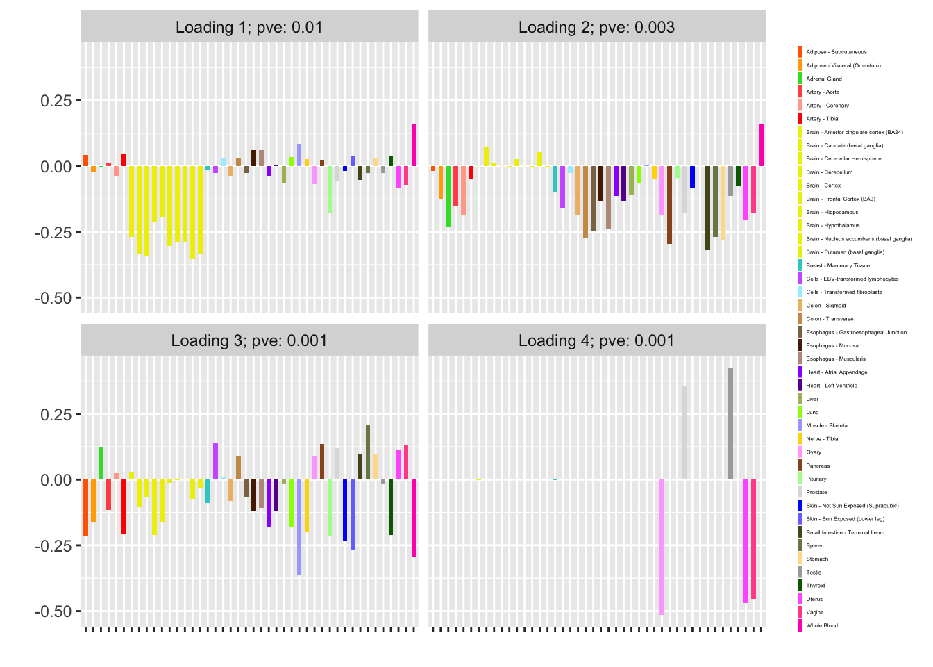

Nonnegative loadings are not as compelling (but I’m not sure that they make much sense in this scenario anyway):

fl_nonneg <- flash_fit(data, 1, var_type = "zero", nonnegative = TRUE)
fl_nonneg$objective
#> [1] -12448.13
plot(fl_nonneg, plot_loadings = TRUE, loading_colors = gtex.colors,
     loading_legend_size = 3, plot_scree = FALSE)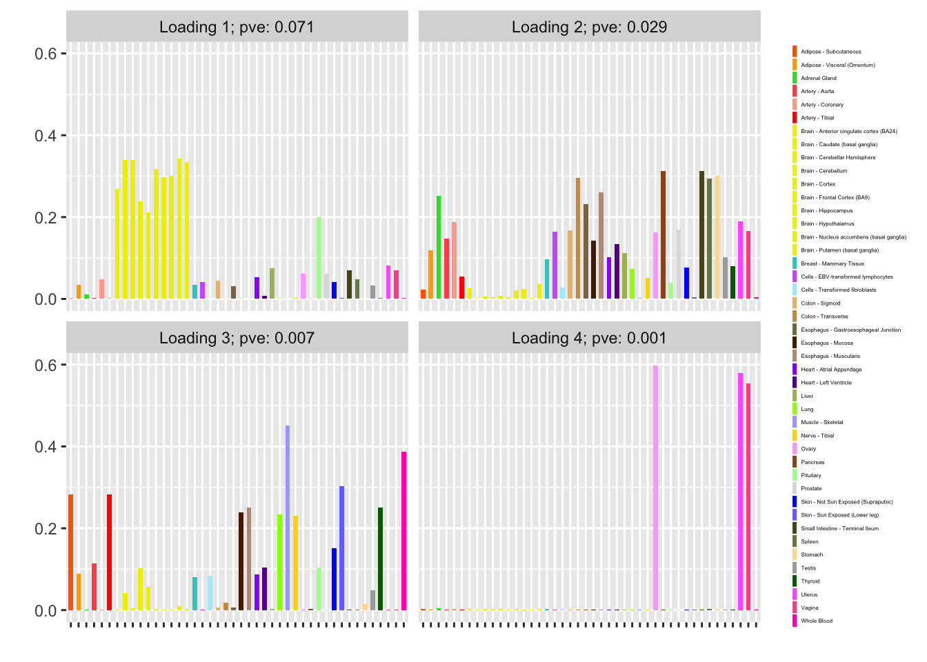

Session information

sessionInfo()
#> R version 3.4.3 (2017-11-30)
#> Platform: x86_64-apple-darwin15.6.0 (64-bit)
#> Running under: macOS High Sierra 10.13.6
#> 
#> Matrix products: default
#> BLAS: /Library/Frameworks/R.framework/Versions/3.4/Resources/lib/libRblas.0.dylib
#> LAPACK: /Library/Frameworks/R.framework/Versions/3.4/Resources/lib/libRlapack.dylib
#> 
#> locale:
#> [1] en_US.UTF-8/en_US.UTF-8/en_US.UTF-8/C/en_US.UTF-8/en_US.UTF-8
#> 
#> attached base packages:
#> [1] stats     graphics  grDevices utils     datasets  methods   base     
#> 
#> other attached packages:
#> [1] ebnm_0.1-15  flashr_0.6-2
#> 
#> loaded via a namespace (and not attached):
#>  [1] Rcpp_0.12.18        pillar_1.2.1        plyr_1.8.4         
#>  [4] compiler_3.4.3      git2r_0.21.0        workflowr_1.0.1    
#>  [7] R.methodsS3_1.7.1   R.utils_2.6.0       iterators_1.0.9    
#> [10] tools_3.4.3         testthat_2.0.0      digest_0.6.15      
#> [13] tibble_1.4.2        evaluate_0.10.1     memoise_1.1.0      
#> [16] gtable_0.2.0        lattice_0.20-35     rlang_0.2.0        
#> [19] Matrix_1.2-12       foreach_1.4.4       commonmark_1.4     
#> [22] yaml_2.1.17         parallel_3.4.3      withr_2.1.1.9000   
#> [25] stringr_1.3.0       roxygen2_6.0.1.9000 xml2_1.2.0         
#> [28] knitr_1.20          REBayes_1.2         devtools_1.13.4    
#> [31] rprojroot_1.3-2     grid_3.4.3          R6_2.2.2           
#> [34] rmarkdown_1.8       reshape2_1.4.3      ggplot2_2.2.1      
#> [37] ashr_2.2-13         magrittr_1.5        whisker_0.3-2      
#> [40] backports_1.1.2     scales_0.5.0        codetools_0.2-15   
#> [43] htmltools_0.3.6     MASS_7.3-48         assertthat_0.2.0   
#> [46] softImpute_1.4      colorspace_1.3-2    labeling_0.3       
#> [49] stringi_1.1.6       Rmosek_7.1.3        lazyeval_0.2.1     
#> [52] doParallel_1.0.11   pscl_1.5.2          munsell_0.4.3      
#> [55] truncnorm_1.0-8     SQUAREM_2017.10-1   R.oo_1.21.0