Nonnegative FLASH example
Jason Willwerscheid
9/11/2018
Last updated: 2018-09-25
workflowr checks: (Click a bullet for more information)-
✔ R Markdown file: up-to-date
Great! Since the R Markdown file has been committed to the Git repository, you know the exact version of the code that produced these results.
-
✔ Environment: empty
Great job! The global environment was empty. Objects defined in the global environment can affect the analysis in your R Markdown file in unknown ways. For reproduciblity it’s best to always run the code in an empty environment.
-
✔ Seed:
set.seed(20180714)The command
set.seed(20180714)was run prior to running the code in the R Markdown file. Setting a seed ensures that any results that rely on randomness, e.g. subsampling or permutations, are reproducible. -
✔ Session information: recorded
Great job! Recording the operating system, R version, and package versions is critical for reproducibility.
-
Great! You are using Git for version control. Tracking code development and connecting the code version to the results is critical for reproducibility. The version displayed above was the version of the Git repository at the time these results were generated.✔ Repository version: f3e1061
Note that you need to be careful to ensure that all relevant files for the analysis have been committed to Git prior to generating the results (you can usewflow_publishorwflow_git_commit). workflowr only checks the R Markdown file, but you know if there are other scripts or data files that it depends on. Below is the status of the Git repository when the results were generated:
Note that any generated files, e.g. HTML, png, CSS, etc., are not included in this status report because it is ok for generated content to have uncommitted changes.Ignored files: Ignored: .DS_Store Ignored: .Rhistory Ignored: .Rproj.user/ Ignored: docs/.DS_Store Ignored: docs/figure/.DS_Store Untracked files: Untracked: data/greedy19.rds
Expand here to see past versions:
| File | Version | Author | Date | Message |
|---|---|---|---|---|
| Rmd | f3e1061 | Jason Willwerscheid | 2018-09-25 | wflow_publish(“analysis/nonnegative.Rmd”) |
| html | f973901 | Jason Willwerscheid | 2018-09-18 | Build site. |
| html | 7720e0b | Jason Willwerscheid | 2018-09-12 | Build site. |
| html | 1f23415 | Jason Willwerscheid | 2018-09-12 | Build site. |
| Rmd | 25f8ad5 | Jason Willwerscheid | 2018-09-12 | wflow_publish(“analysis/nonnegative.Rmd”) |
| html | 2825464 | Jason Willwerscheid | 2018-09-11 | Build site. |
| Rmd | 89b711c | Jason Willwerscheid | 2018-09-11 | wflow_publish(“analysis/nonnegative.Rmd”) |
Introduction
Nonnegative matrix factorization is straightforward in FLASH; we need only put a class of nonnegative priors on the factors and loadings. In ASH, the +uniform priors constitute such a class (and, at present, this is the only such class in ASH).
As an example of nonnegative matrix factorization via FLASH, I analyze the GTEx donation matrix. This matrix consists of 44 rows, each of which corresponds to a tissue or cell type (liver, lung, cortex, whole blood, etc.), and 571 columns, each of which corresponds to a donor. Note that a given donor can contribute multiple samples of a given tissue.
In this analysis, I ignore the fact that “errors” are not, as FLASH assumes, Gaussian. I will address this simplification in subsequent analyses (see here and here).
Data
First I set up the donation matrix. As in previous analyses, I use GTEx v6 data rather than the more recent v7 or v8 data.
raw <- read.csv("https://storage.googleapis.com/gtex_analysis_v6/annotations/GTEx_Data_V6_Annotations_SampleAttributesDS.txt",
                header=TRUE, sep='\t')

data <- raw[, c("SAMPID", "SMTSD")] # sample ID, tissue type
# Extract donor ID:
tmp <- strsplit(as.character(data$SAMPID), "-")
data$SAMPID <- as.factor(sapply(tmp, function(x) {x[[2]]}))
names(data) <- c("DonorID", "TissueType")

data <- suppressMessages(reshape2::acast(data, TissueType ~ DonorID))

missing.tissues <- c(1, 8, 9, 20, 21, 24, 26, 27, 33, 36, 39)
data <- data[-missing.tissues, ]

gtex.colors <- read.table("https://github.com/stephenslab/gtexresults/blob/master/data/GTExColors.txt?raw=TRUE",
                          sep = '\t', comment.char = '')
gtex.colors <- gtex.colors[-c(7, 8, 19, 20, 24, 25, 31, 34, 37), 2]
gtex.colors <- as.character(gtex.colors)
As a preliminary step, it is useful to visualize the correlation matrix. I use Kushal Dey’s CorShrink package, which outputs the empirical correlation matrix and shrunken estimates of the “true” correlations.
tmp <- capture.output(
  CorShrink::CorShrinkData(t(data), sd_boot = TRUE, image = "both",
                           image.control = list(tl.cex = 0.25))
)
Using sd_boot as value column: use value.var to override.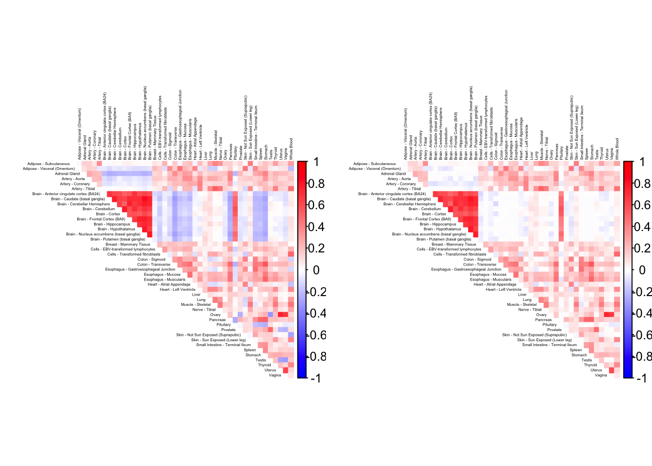
Expand here to see past versions of corr-1.png:
| Version | Author | Date |
|---|---|---|
| 1f23415 | Jason Willwerscheid | 2018-09-12 |
Initialization function
To obtain nonnegative factor/loading pairs using FLASH, we can likely do better than to use the default SVD-type initialization. Here I use the nonnegative matrix factorization implemented in package NNLM.
udv_nn = function(Y, K = 1) {
  tmp = NNLM::nnmf(Y, K, verbose = FALSE)
  return(list(d = rep(1, K), u = tmp$W, v = t(tmp$H)))
}
Greedy loadings
One round of greedily adding factors and then backfitting produces five factor/loading pairs, but repeated rounds yield additional factor/loadings. Here I do three rounds of fitting. I obtain the following loadings:
devtools::load_all("~/GitHub/flashr")Loading flashrdevtools::load_all("~/GitHub/ebnm")Loading ebnmebnm_fn = "ebnm_ash"
ebnm_param = list(mixcompdist = "+uniform", warmstart = TRUE)
run_flash_once <- function(f_init) {
flash(data, f_init = f_init,
ebnm_fn = ebnm_fn, ebnm_param = ebnm_param,
var_type="constant", init_fn = udv_nn,
backfit = TRUE, verbose = FALSE)
}
fl_g <- run_flash_once(f_init = NULL)
fl_g <- run_flash_once(f_init = fl_g)
fl_g <- run_flash_once(f_init = fl_g)
fl_g$objective[1] -15156.65plot(fl_g, plot_loadings = TRUE, loading_colors = gtex.colors,
loading_legend_size = 3,
plot_grid_nrow = 4, plot_grid_ncol = 3)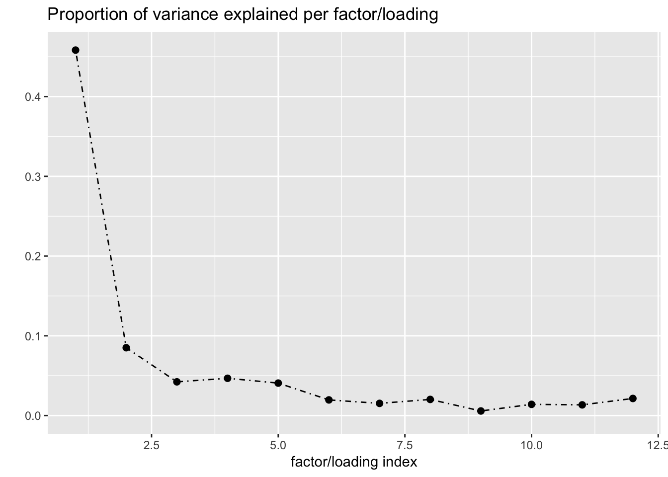
Expand here to see past versions of greedy-1.png:
| Version | Author | Date |
|---|---|---|
| 2825464 | Jason Willwerscheid | 2018-09-11 |
Backfitted loadings
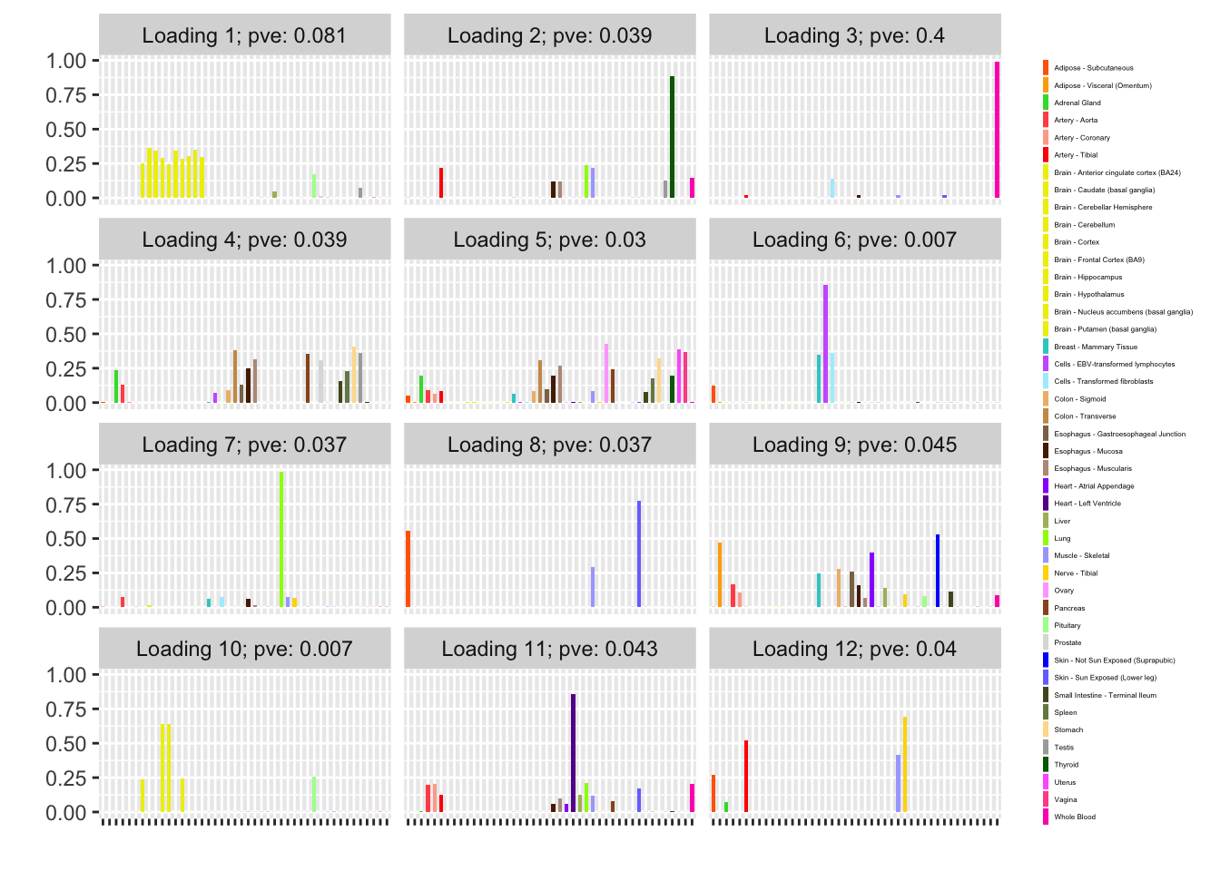
Next I add 12 factors at once using NNLM and then backfit. Note that the objective obtained using this method is much better than the above (by approximately 500).
fl_nnmf <- flash_add_factors_from_data(data, 12,
                                       init_fn = udv_nn,
                                       backfit = FALSE)

fl_b <- flash_backfit(data, fl_nnmf,
                      ebnm_fn = ebnm_fn,
                      ebnm_param = ebnm_param,
                      var_type = "constant",
                      verbose = FALSE)
fl_b$objective
[1] -14666.36plot(fl_b, plot_loadings = TRUE, loading_colors = gtex.colors,
loading_legend_size = 3,
plot_grid_nrow = 4, plot_grid_ncol = 3)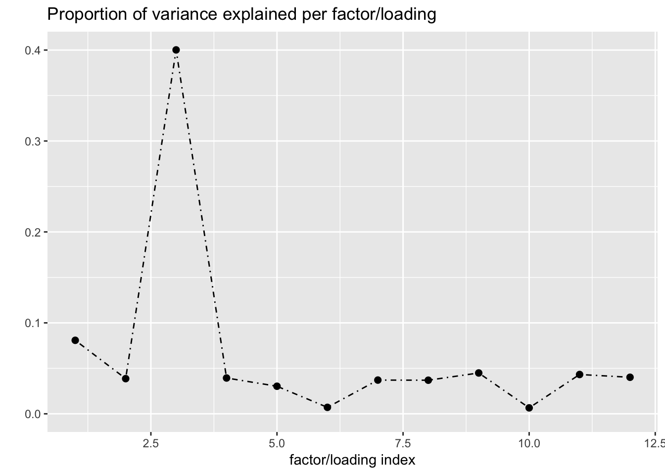
Expand here to see past versions of backfit-1.png:
| Version | Author | Date |
|---|---|---|
| 2825464 | Jason Willwerscheid | 2018-09-11 |
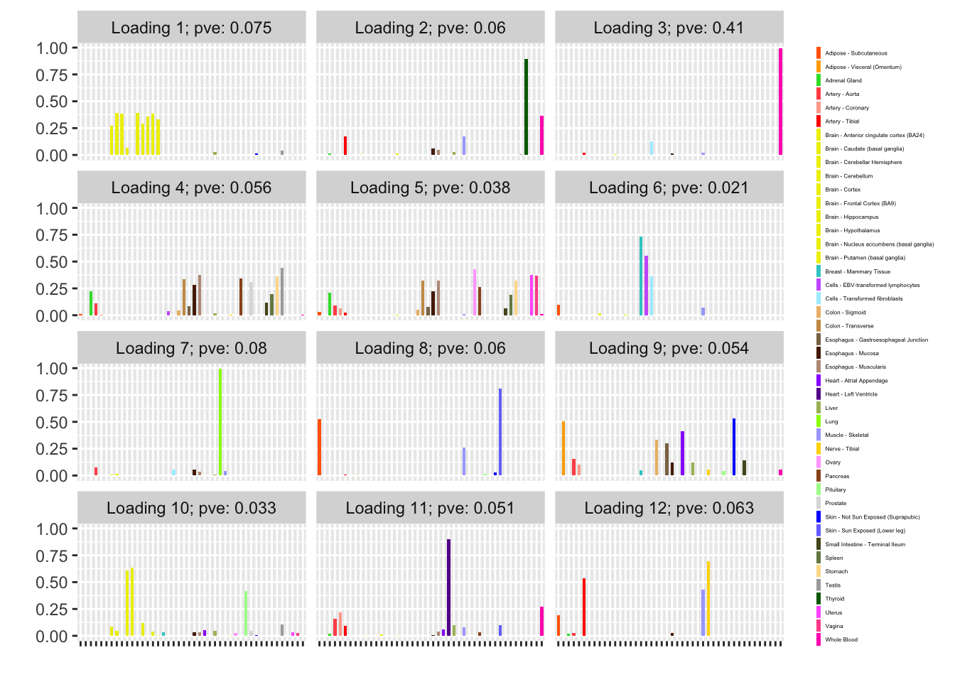
NNLM loadings
The backfitted loadings can be compared with the loadings that are obtained by simply running NNLM. Results are quite similar.
plot(fl_nnmf, plot_loadings=TRUE, loading_colors = gtex.colors,
     loading_legend_size = 3,
     plot_grid_nrow = 4, plot_grid_ncol = 3)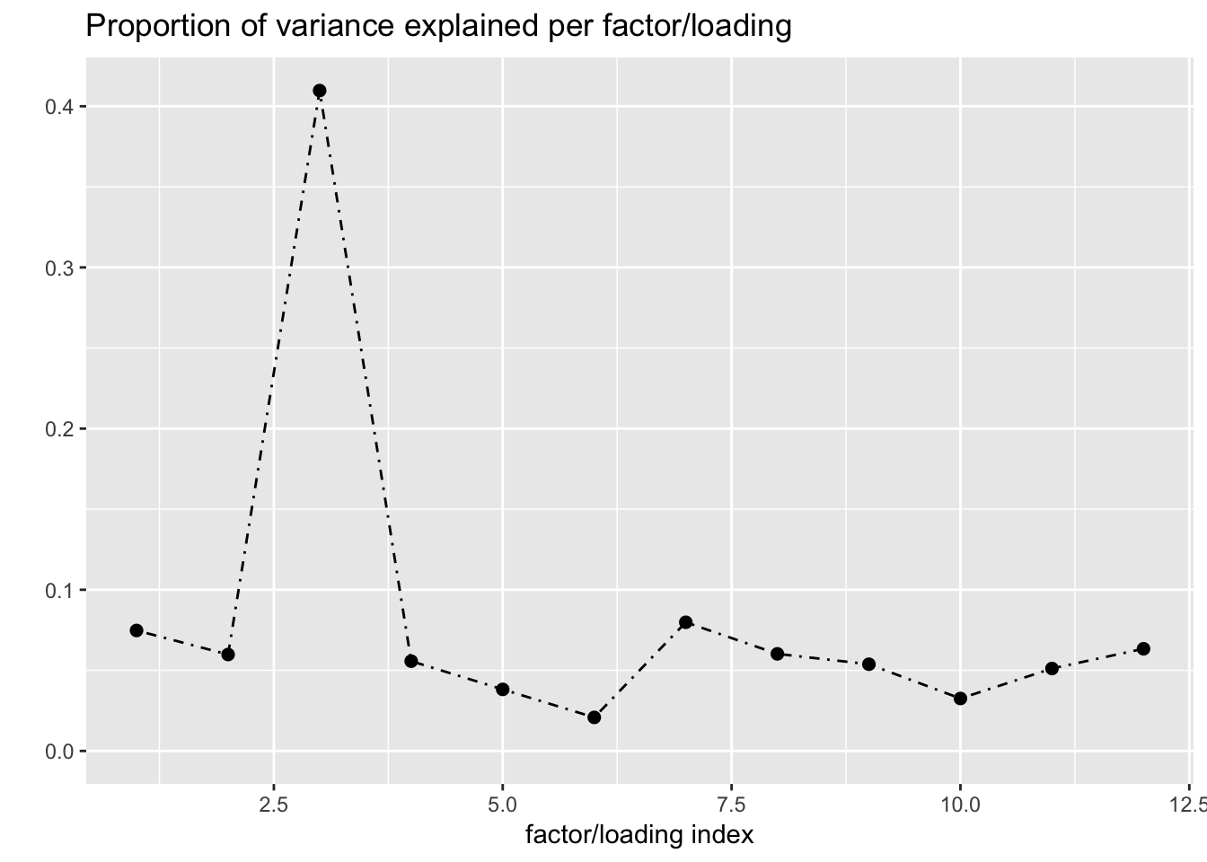
Expand here to see past versions of nnmf-1.png:
| Version | Author | Date |
|---|---|---|
| 2825464 | Jason Willwerscheid | 2018-09-11 |
Discussion
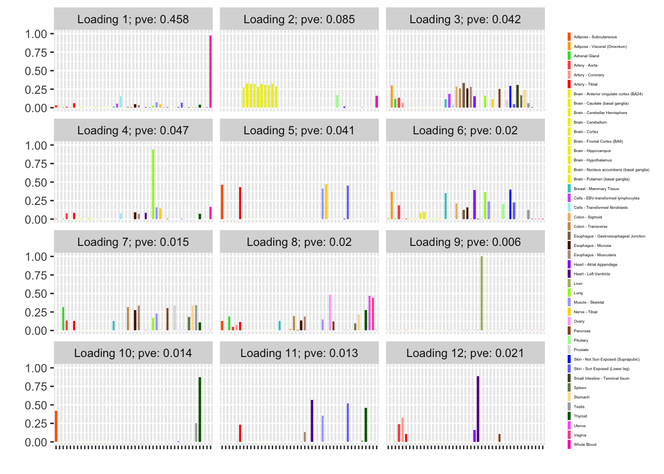
The loading that accounts for the largest PVE (backfitted loading 3) puts a large weight on whole blood and a smaller weight on fibroblasts. In effect, there are many more whole blood samples than samples from any other tissue (1822 versus, on average, 224).
The loading with the second-largest PVE (loading 1) shares weights among brain tissues, with a smaller weight on pituitary tissues. FLASH finds a very similar loading in the GTEx summary data (loading 2 here, for example).
Loading 5 puts large weights on female reproductive tissues (ovary, uterus, and vagina), so it is most likely a sex-specific loading. Similarly, loading 4 puts its largest weights on testicular and prostate tissues. Both of these loadings put very similar weights on non-reproductive tissues (observe, in particular, the similarity of weights among gastro-intestinal tissues), so we should not make too much of correlations between reproductive and non-reproductive tissues. It is probably the case that the two sex-specific loadings are entangled with a third loading that is more properly weighted on gastro-intestinal tissues alone.
Session information
sessionInfo()R version 3.4.3 (2017-11-30)
Platform: x86_64-apple-darwin15.6.0 (64-bit)
Running under: macOS High Sierra 10.13.6
Matrix products: default
BLAS: /Library/Frameworks/R.framework/Versions/3.4/Resources/lib/libRblas.0.dylib
LAPACK: /Library/Frameworks/R.framework/Versions/3.4/Resources/lib/libRlapack.dylib
locale:
[1] en_US.UTF-8/en_US.UTF-8/en_US.UTF-8/C/en_US.UTF-8/en_US.UTF-8
attached base packages:
[1] stats graphics grDevices utils datasets methods base
other attached packages:
[1] ebnm_0.1-15 flashr_0.6-2
loaded via a namespace (and not attached):
[1] softImpute_1.4 NNLM_0.4.2 ashr_2.2-13
[4] reshape2_1.4.3 corrplot_0.84 lattice_0.20-35
[7] Rmosek_7.1.3 colorspace_1.3-2 testthat_2.0.0
[10] htmltools_0.3.6 yaml_2.1.17 rlang_0.2.0
[13] R.oo_1.21.0 pillar_1.2.1 withr_2.1.1.9000
[16] R.utils_2.6.0 REBayes_1.2 foreach_1.4.4
[19] plyr_1.8.4 stringr_1.3.0 munsell_0.4.3
[22] commonmark_1.4 gtable_0.2.0 workflowr_1.0.1
[25] R.methodsS3_1.7.1 devtools_1.13.4 codetools_0.2-15
[28] memoise_1.1.0 evaluate_0.10.1 labeling_0.3
[31] knitr_1.20 pscl_1.5.2 doParallel_1.0.11
[34] parallel_3.4.3 Rcpp_0.12.18 corpcor_1.6.9
[37] backports_1.1.2 scales_0.5.0 truncnorm_1.0-8
[40] gridExtra_2.3 ggplot2_2.2.1 digest_0.6.15
[43] stringi_1.1.6 grid_3.4.3 rprojroot_1.3-2
[46] tools_3.4.3 magrittr_1.5 lazyeval_0.2.1
[49] glmnet_2.0-13 CorShrink_0.1-6 tibble_1.4.2
[52] whisker_0.3-2 MASS_7.3-48 Matrix_1.2-12
[55] SQUAREM_2017.10-1 xml2_1.2.0 assertthat_0.2.0
[58] rmarkdown_1.8 roxygen2_6.0.1.9000 iterators_1.0.9
[61] R6_2.2.2 git2r_0.21.0 compiler_3.4.3 This reproducible R Markdown analysis was created with workflowr 1.0.1