Montoro et al. droplet dataset analysis

Introduction

Here I explore a 30-factor flashier object that was fitted using the lessons learned from the previous analyses:

1. I scale the raw counts \(X_{ij}\) using cell-wise size factors \(\lambda_j\) estimated via Aaron Lun’s R package scran (normalizing so that the median size factor is equal to one).

2. I divide the scaled counts by the pseudocount \(\alpha = 0.5\), add 1, and take logs to obtain \(Y_{ij} = \log \left(\frac{X_{ij}}{\alpha\lambda_j} + 1 \right)\). Note that this is equivalent to adding \(\alpha\) and taking logs (up to an additive constant), but it preserves sparsity.

3. It’s best to account for heteroskedasticity among both cells and genes. This can be done by estimating cell-wise variances in advance, scaling the log-transformed counts, and then fitting a flashier object to the matrix \(Y_{ij} / \hat{\sigma}_j\) using a gene-wise variance structure.

4. To aid interpretability, I use semi-nonnegative priors with non-negative priors on cells.

5. I perform a final backfit, which accounts for by far the largest portion of the 3.4 hours needed. If fitting time were an issue, I’d consider limiting the number of backfitting iterations. Here, 180 backfitting iterations were performed, but I suspect that one could get a reasonably good fit with maxiter as few as 10.

The code used to produce the fit can be viewed here.

source("./code/utils.R")
droplet <- readRDS("./data/droplet.rds")
droplet <- preprocess.droplet(droplet)

res <- readRDS("./output/final_montoro/final_fit.rds")

Overview

I first plot the factors in the order they were added.

plot.factors(res, droplet$cell.type, 1:res$fl$n.factors, nonnegative = TRUE)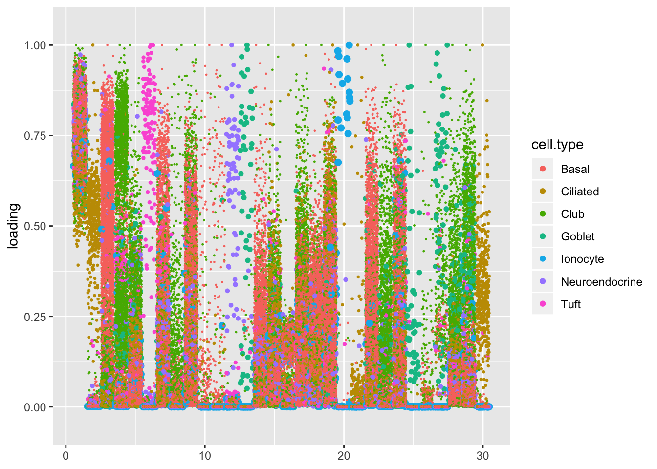

A heatmap of the correlation matrix \(F^T F\) (where \(F\) is the matrix of \(\ell_2\)-normalized cell loadings) can usefully orient a discussion of the results.

heat <- heatmap(crossprod(res$fl$loadings.pm[[2]]))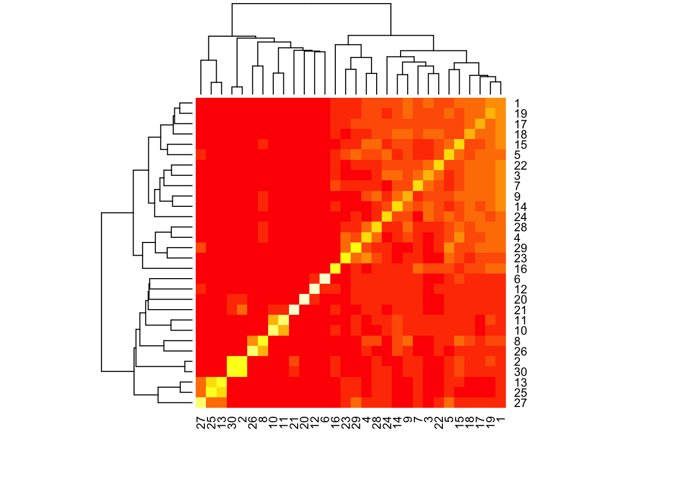

I re-order the factors to match the order given in the heatmap. The first branch of the dendrogram separates a large mass of club and basal cells from more specialized cell types. From left to right, there are easily identifiable clusters of goblet cells, ciliated cells, hillock cells, a small subset of basal cells, more ciliated cells, ionocytes, neuroendocrine cells, and tuft cells. Among the mass of club and basal cells, one can distinguish a lone factor that’s primarily loaded on genes that code for ribosomal proteins (Factor 16), four factors loaded on club cells, six factors loaded on basal cells, and six factors that are a wintry mix of cell types.

plot.factors(res, droplet$cell.type, heat$rowInd, nonnegative = TRUE)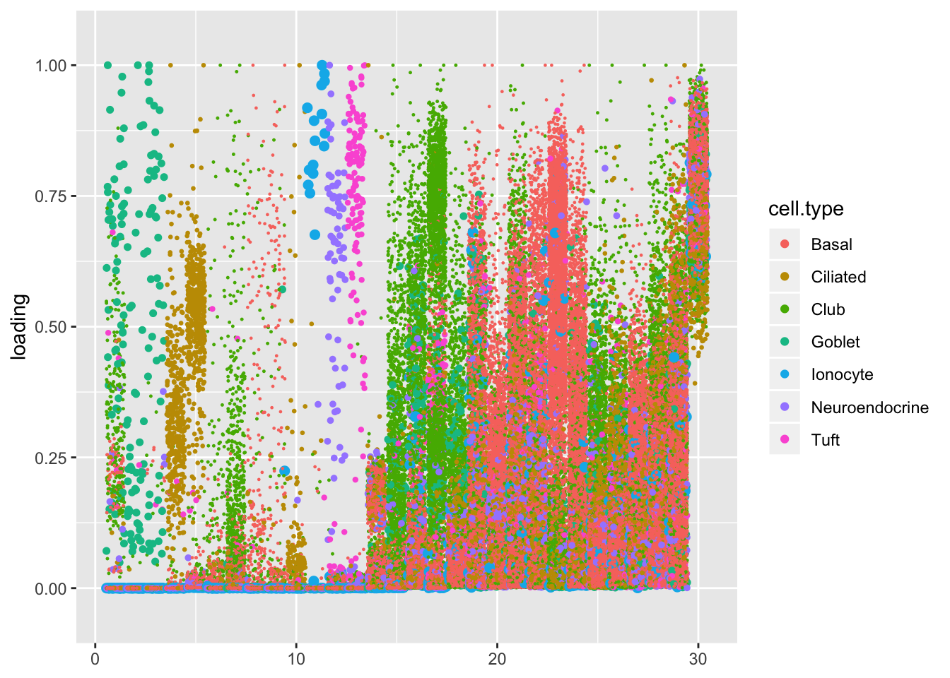

Goblet factors

Factors 13 and 25 nicely distinguish among the “goblet-1” and “goblet-2” subpopulations identified by Montoro et al. (Genes that mark goblet-1 cells are indicated in blue, while goblet-2 marker genes are in red.) I’m not sure what factor 27 is doing. It’s possible that it is indexing cellular functions that are distributed among goblet cells and other cell types (primarily club), but it’s also possible that it is an artefact caused by incomplete convergence.

top.n <- 50
label.top.n <- 20
plot.one.factor(res$fl, 13, droplet$all.goblet.genes,
                title = "Factor 13 (goblet)", gene.colors = droplet$all.goblet.colors,
                top.n = top.n, label.top.n = label.top.n)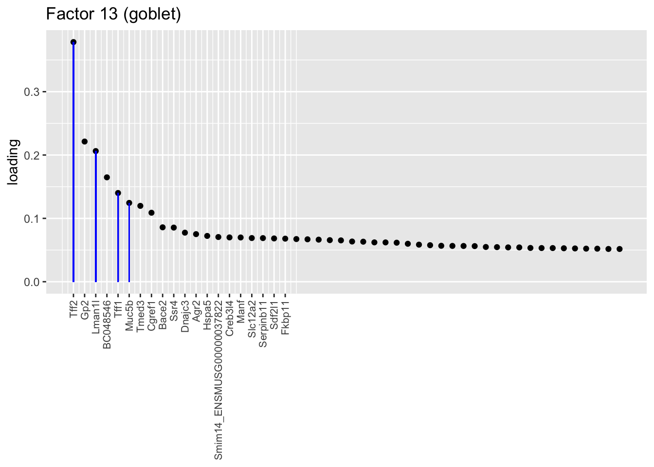

plot.one.factor(res$fl, 25,droplet$all.goblet.genes,
                title = "Factor 25 (goblet)", gene.colors = droplet$all.goblet.colors,
                top.n = top.n, label.top.n = label.top.n)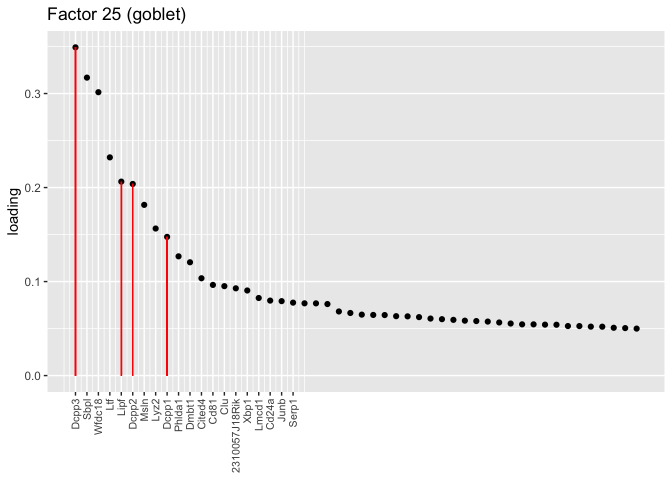

plot.one.factor(res$fl, 27, droplet$all.goblet.genes,
                title = "Factor 27 (goblet)", gene.colors = droplet$all.goblet.colors,
                top.n = top.n, label.top.n = label.top.n)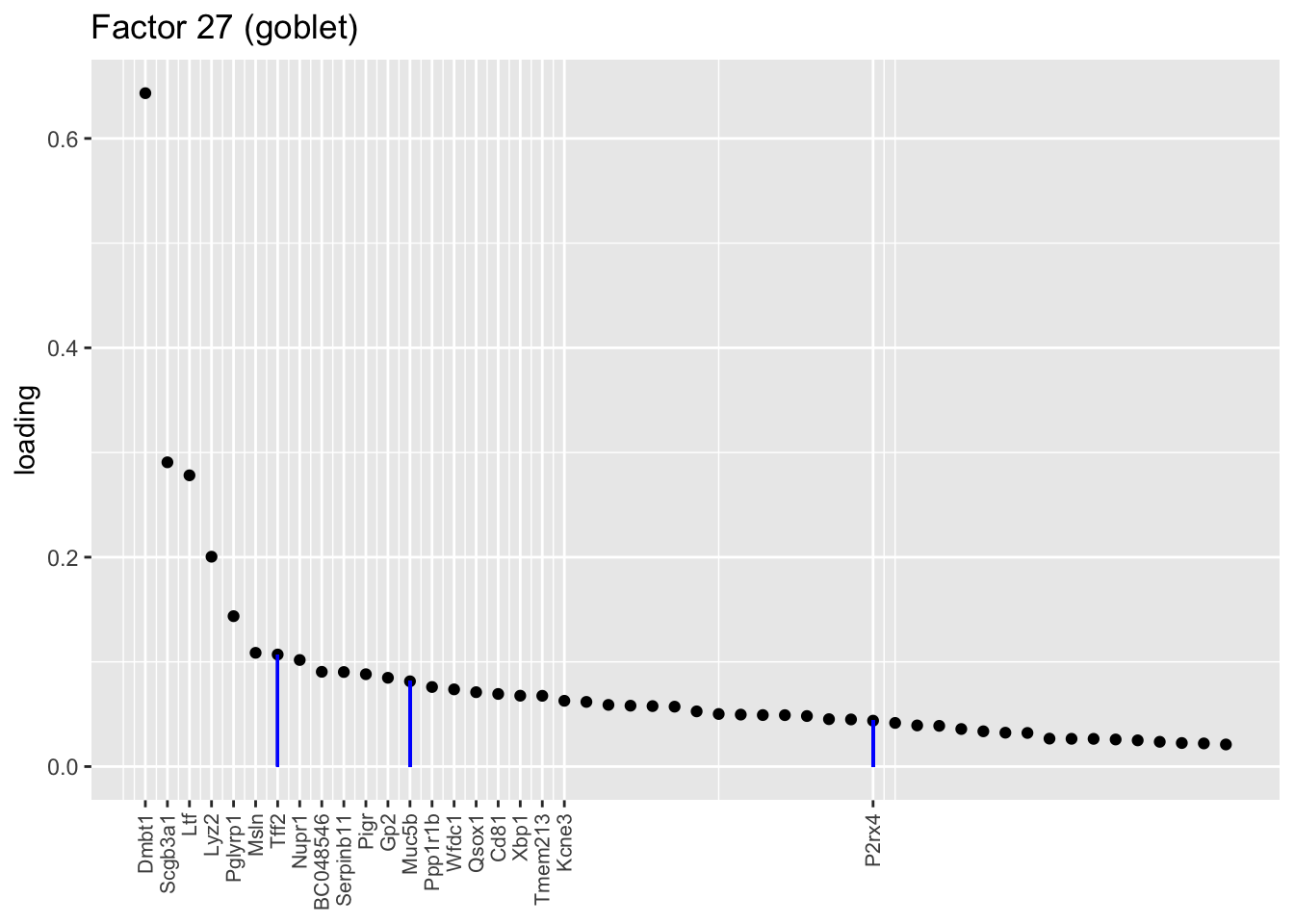

Ciliated factors

I don’t know enough to go into detail, but the two ciliated factors are clearly indexing two very different gene sets.

plot.one.factor(res$fl, 2, NULL,
                title = "Factor 2 (ciliated)",
                top.n = top.n, label.top.n = label.top.n)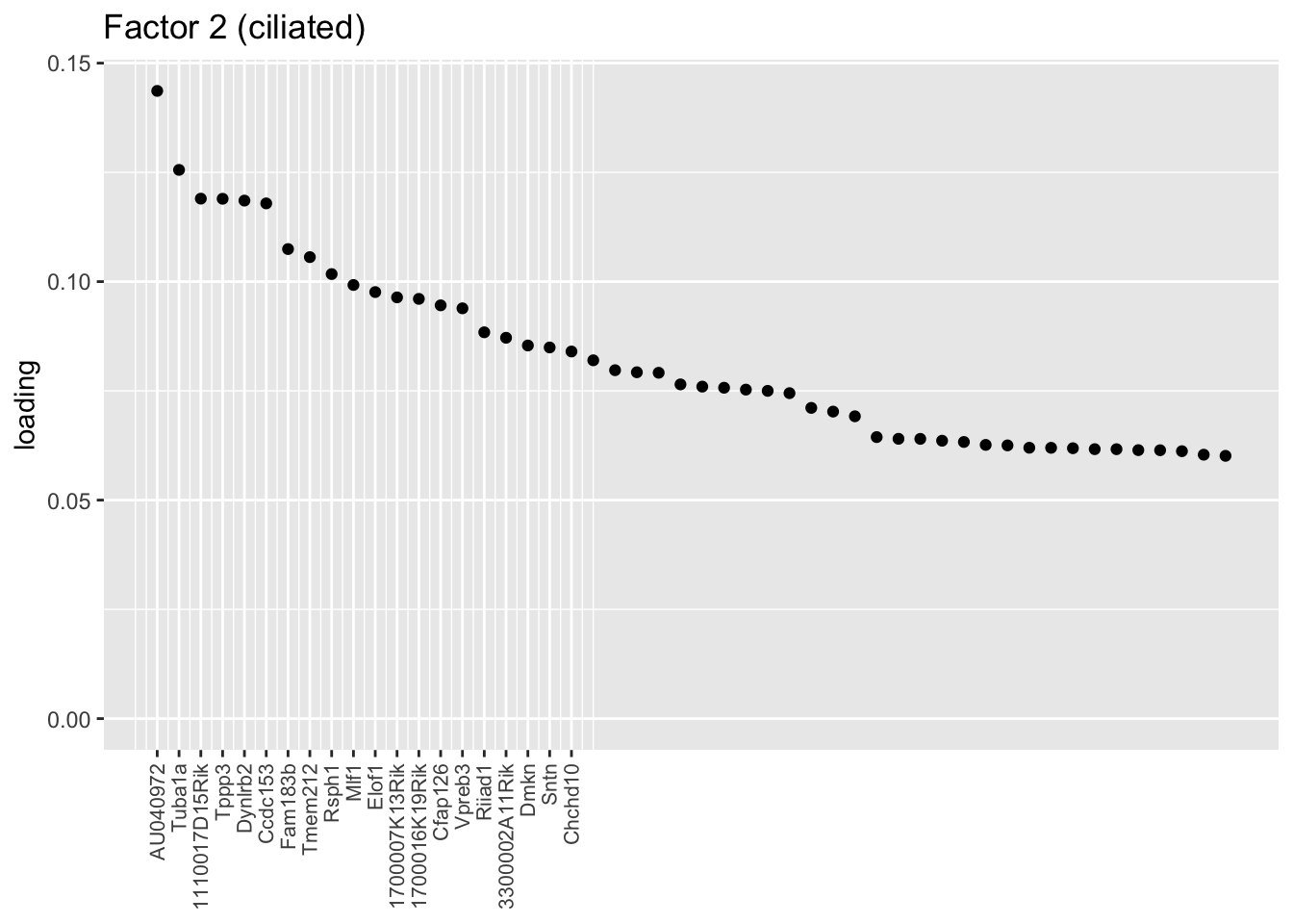

plot.one.factor(res$fl, 30, NULL,
                title = "Factor 30 (ciliated)",
                top.n = top.n, label.top.n = label.top.n)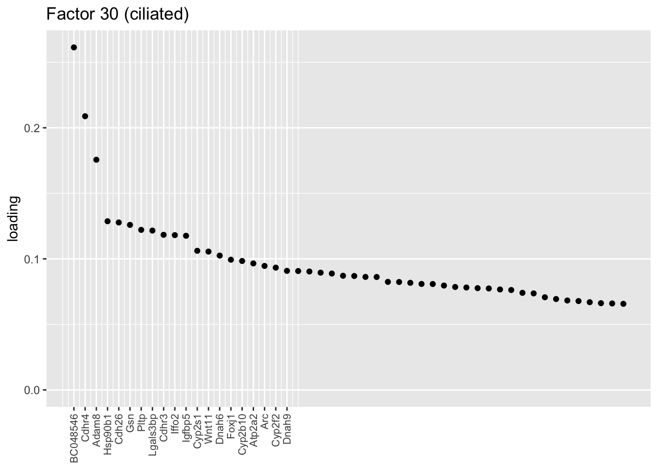

A third ciliated factor (Factor 10) doesn’t cluster with the other two, and indexes yet another ciliated-specific gene set.

plot.one.factor(res$fl, 10, NULL,
                title = "Factor 10 (ciliated)",
                top.n = top.n, label.top.n = label.top.n)

Hillock factors

One feature that is identified in the pulse-seq dataset but not the droplet-based dataset is a subpopulation of transitional cells along the basal-to-club trajectory organized in “hillocks.” Factor 8 turns out to be the factor with largest mean loading among genes that Montoro et al. identify as particularly highly expressed in hillock cells (indicated below in red). Factor 14, included among the basal factors, is also highly loaded on many of these genes. I’d conjecture that Factor 8 (which clusters with Factor 26) picks out cells nearer to the club end of the trajectory, while 14 picks out cells nearer to the basal end.

plot.one.factor(res$fl, 8, droplet$hillock.genes, 
                title = "Factor 8 (club-hillock)", 
                top.n = top.n, label.top.n = 10)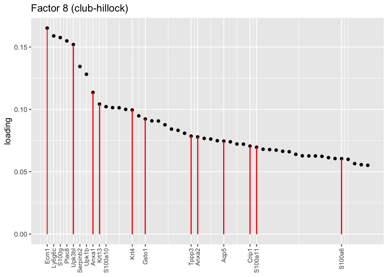

plot.one.factor(res$fl, 26, droplet$hillock.genes, 
                title = "Factor 26 (club-hillock)", 
                top.n = 60, label.top.n = 10)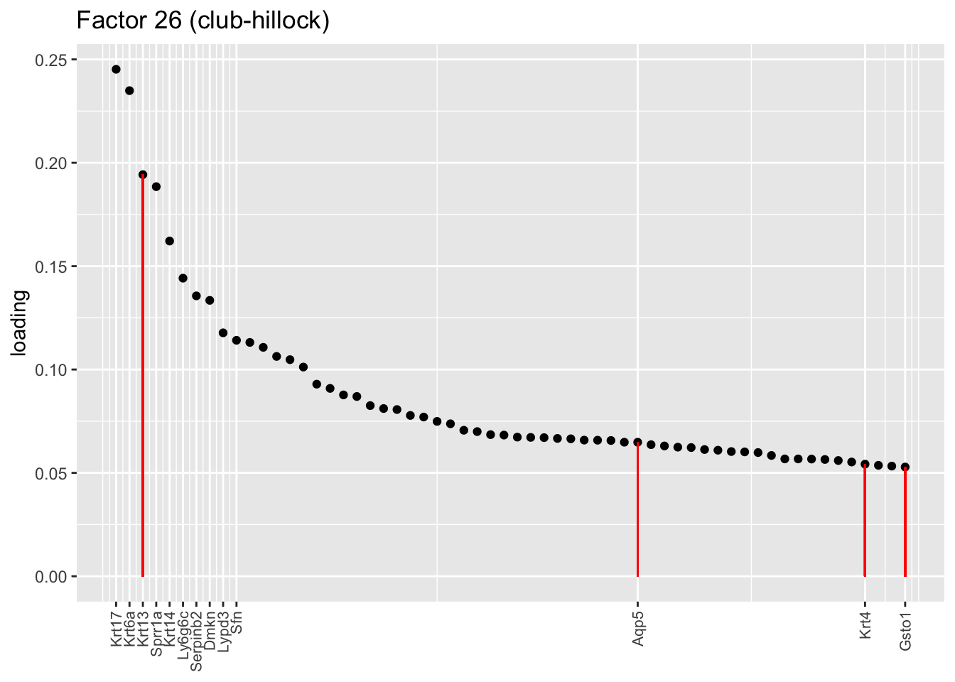

plot.one.factor(res$fl, 14, droplet$hillock.genes, 
                title = "Factor 14 (basal-hillock)", 
                top.n = top.n, label.top.n = 10)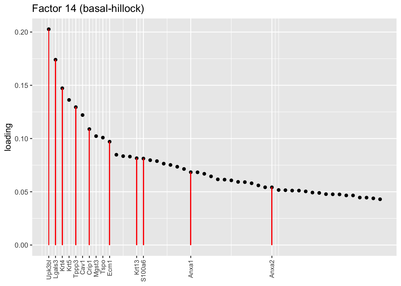

Sparse basal factors

The next cluster is comprised of a small subset of basal cells. I don’t have much to say about it, except that many of the top genes are also highly expressed in ciliated cells, so it’s possible that these are basal cells that have begun to differentiate into ciliated cells.

plot.one.factor(res$fl, 10, NULL,
                title = "Factor 10 (basal)", 
                top.n = top.n, label.top.n = label.top.n)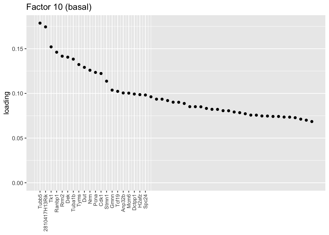

plot.one.factor(res$fl, 11, NULL,
                title = "Factor 11 (basal)", 
                top.n = top.n, label.top.n = label.top.n)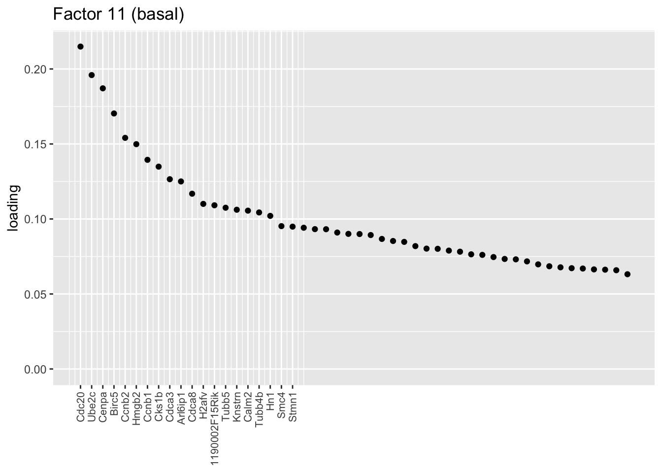

Ionocytes, neuroendocrine cells, tuft cells

These are each relatively clean factors that are specific to a single cell type. The tuft factor does not distinguish between tuft-1 (blue) and tuft-2 (red) subpopulations.

plot.one.factor(res$fl, 20, droplet$ionocyte.genes, 
                title = "Factor 20 (ionocytes)", 
                top.n = 70, label.top.n = 9)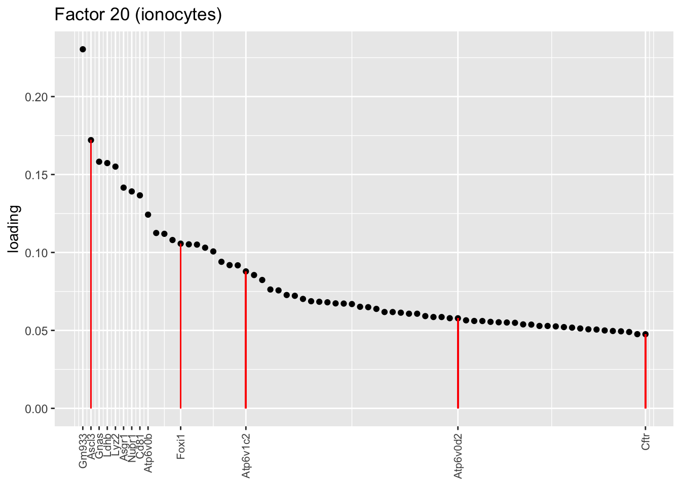

plot.one.factor(res$fl, 12, NULL, 
                title = "Factor 12 (neuroendocrine)", 
                top.n = top.n, label.top.n = label.top.n)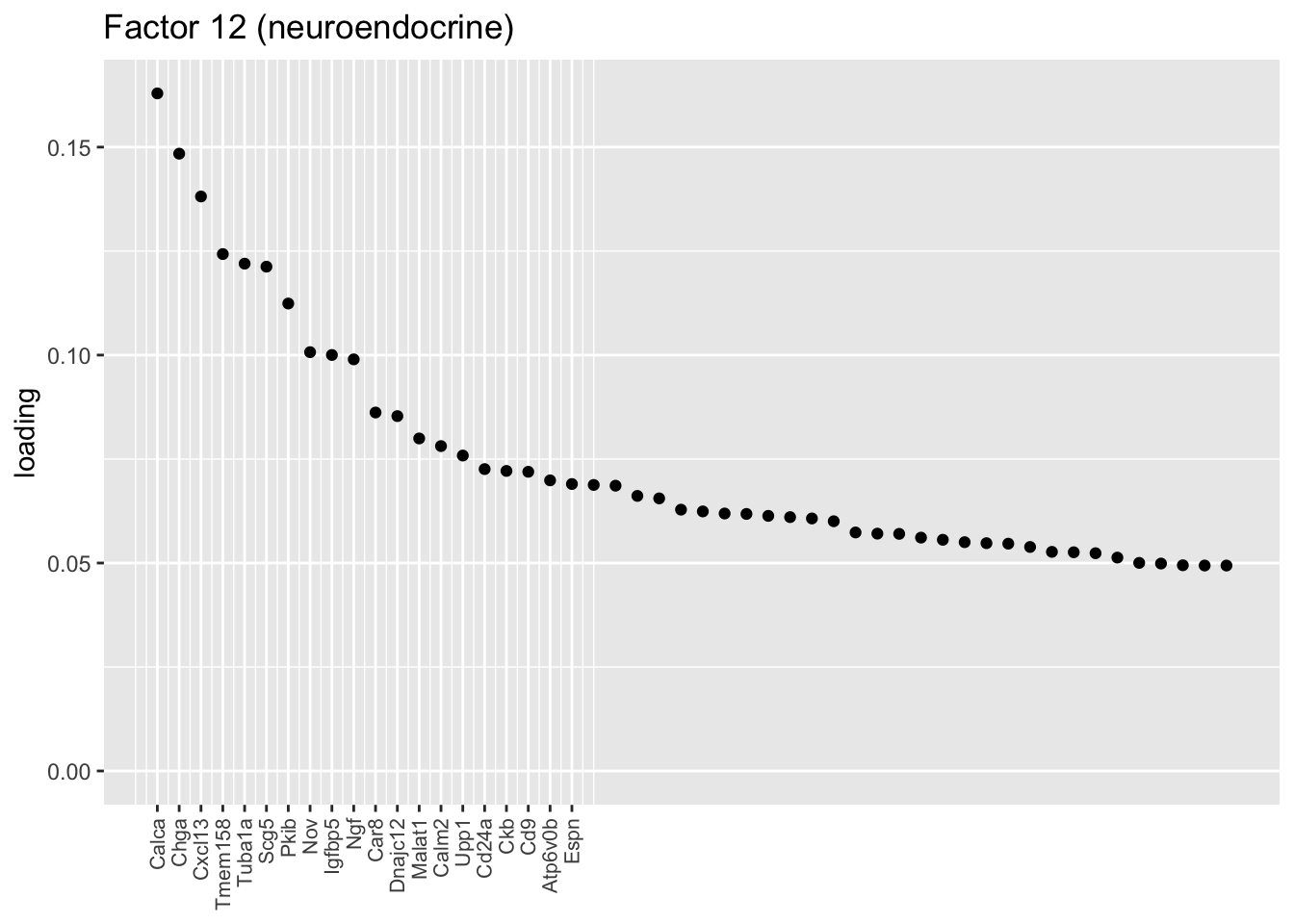

plot.one.factor(res$fl, 6, droplet$all.tuft.genes, 
                title = "Factor 6 (tuft)", gene.colors = droplet$all.tuft.colors,
                top.n = 100, label.top.n = 4)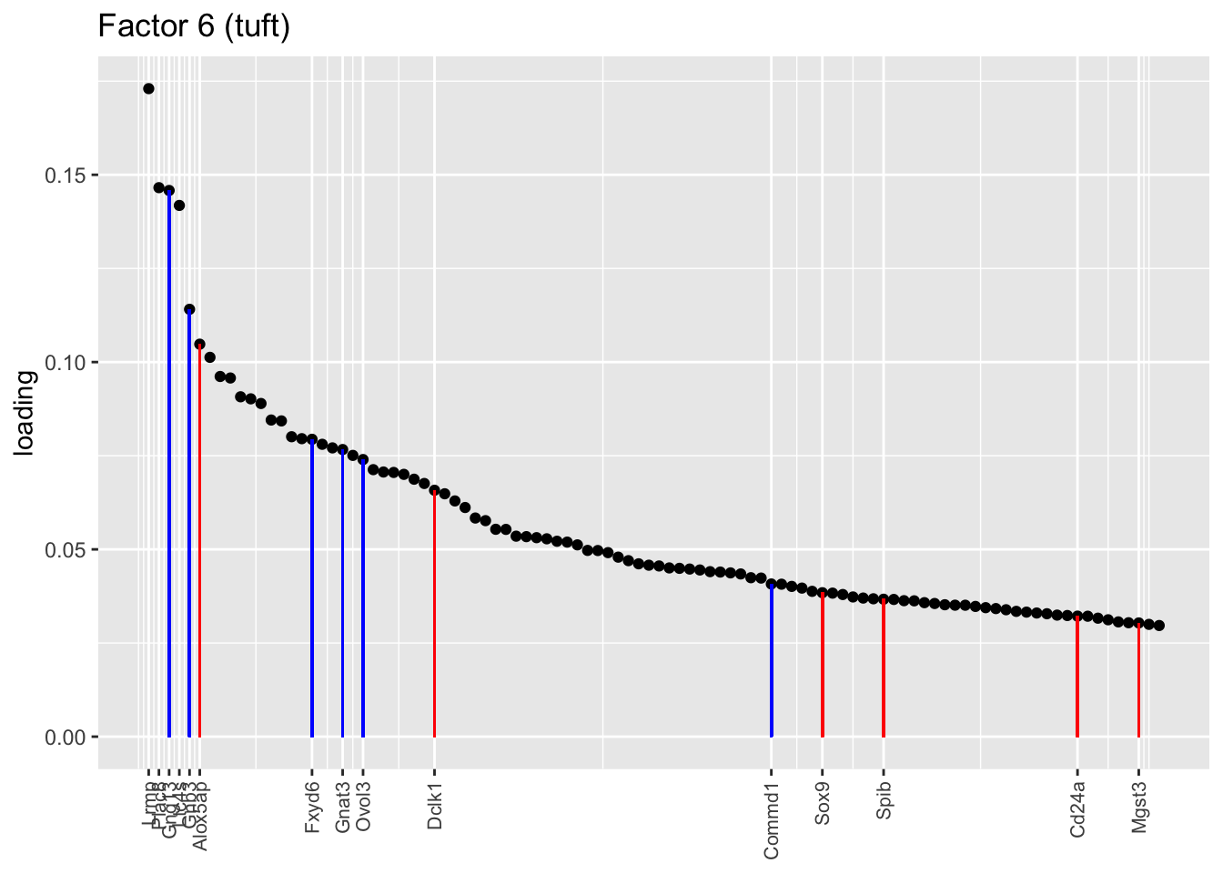

Session information

sessionInfo()

R version 3.5.3 (2019-03-11)
Platform: x86_64-apple-darwin15.6.0 (64-bit)
Running under: macOS Mojave 10.14.6

Matrix products: default
BLAS: /Library/Frameworks/R.framework/Versions/3.5/Resources/lib/libRblas.0.dylib
LAPACK: /Library/Frameworks/R.framework/Versions/3.5/Resources/lib/libRlapack.dylib

locale:
[1] en_US.UTF-8/en_US.UTF-8/en_US.UTF-8/C/en_US.UTF-8/en_US.UTF-8

attached base packages:
[1] stats     graphics  grDevices utils     datasets  methods   base     

other attached packages:
[1] flashier_0.1.17 ggplot2_3.2.0   Matrix_1.2-15  

loaded via a namespace (and not attached):
 [1] Rcpp_1.0.1        plyr_1.8.4        compiler_3.5.3   
 [4] pillar_1.3.1      git2r_0.25.2      workflowr_1.2.0  
 [7] iterators_1.0.10  tools_3.5.3       digest_0.6.18    
[10] evaluate_0.13     tibble_2.1.1      gtable_0.3.0     
[13] lattice_0.20-38   pkgconfig_2.0.2   rlang_0.3.1      
[16] foreach_1.4.4     parallel_3.5.3    yaml_2.2.0       
[19] ebnm_0.1-24       xfun_0.6          withr_2.1.2      
[22] stringr_1.4.0     dplyr_0.8.0.1     knitr_1.22       
[25] fs_1.2.7          rprojroot_1.3-2   grid_3.5.3       
[28] tidyselect_0.2.5  glue_1.3.1        R6_2.4.0         
[31] rmarkdown_1.12    mixsqp_0.1-119    reshape2_1.4.3   
[34] ashr_2.2-38       purrr_0.3.2       magrittr_1.5     
[37] whisker_0.3-2     MASS_7.3-51.1     codetools_0.2-16 
[40] backports_1.1.3   scales_1.0.0      htmltools_0.3.6  
[43] assertthat_0.2.1  colorspace_1.4-1  labeling_0.3     
[46] stringi_1.4.3     pscl_1.5.2        doParallel_1.0.14
[49] lazyeval_0.2.2    munsell_0.5.0     truncnorm_1.0-8  
[52] SQUAREM_2017.10-1 crayon_1.3.4