Prior families
Jason Willwerscheid
3/18/2020
Last updated: 2020-03-18
Checks: 6 0
Knit directory: scFLASH/
This reproducible R Markdown analysis was created with workflowr (version 1.2.0). The Report tab describes the reproducibility checks that were applied when the results were created. The Past versions tab lists the development history.
Great! Since the R Markdown file has been committed to the Git repository, you know the exact version of the code that produced these results.
Great job! The global environment was empty. Objects defined in the global environment can affect the analysis in your R Markdown file in unknown ways. For reproduciblity it’s best to always run the code in an empty environment.
The command set.seed(20181103) was run prior to running the code in the R Markdown file. Setting a seed ensures that any results that rely on randomness, e.g. subsampling or permutations, are reproducible.
Great job! Recording the operating system, R version, and package versions is critical for reproducibility.
Nice! There were no cached chunks for this analysis, so you can be confident that you successfully produced the results during this run.
Great! You are using Git for version control. Tracking code development and connecting the code version to the results is critical for reproducibility. The version displayed above was the version of the Git repository at the time these results were generated.
Note that you need to be careful to ensure that all relevant files for the analysis have been committed to Git prior to generating the results (you can use wflow_publish or wflow_git_commit). workflowr only checks the R Markdown file, but you know if there are other scripts or data files that it depends on. Below is the status of the Git repository when the results were generated:
Ignored files:
    Ignored:    .DS_Store
    Ignored:    .Rhistory
    Ignored:    .Rproj.user/
    Ignored:    code/initialization/
    Ignored:    data-raw/10x_assigned_cell_types.R
    Ignored:    data/.DS_Store
    Ignored:    data/10x/
    Ignored:    data/Ensembl2Reactome.txt
    Ignored:    data/droplet.rds
    Ignored:    data/mus_pathways.rds
    Ignored:    output/backfit/
    Ignored:    output/final_montoro/
    Ignored:    output/lowrank/
    Ignored:    output/prior_type/
    Ignored:    output/pseudocount/
    Ignored:    output/pseudocount_redux/
    Ignored:    output/size_factors/
    Ignored:    output/var_reg/
    Ignored:    output/var_type/

Untracked files:
    Untracked:  analysis/NBapprox.Rmd
    Untracked:  analysis/trachea4.Rmd
    Untracked:  code/alt_montoro/
    Untracked:  code/missing_data.R
    Untracked:  code/prior_type/priortype_fits_pbmc.R
    Untracked:  code/pulseseq/
    Untracked:  code/trachea4.R
    Untracked:  mixsqp_fail.rds
    Untracked:  output/alt_montoro/
    Untracked:  output/pulseseq_fit.rds

Unstaged changes:
    Modified:   code/utils.R
    Modified:   data-raw/pbmc.R
Note that any generated files, e.g. HTML, png, CSS, etc., are not included in this status report because it is ok for generated content to have uncommitted changes.
These are the previous versions of the R Markdown and HTML files. If you’ve configured a remote Git repository (see ?wflow_git_remote), click on the hyperlinks in the table below to view them.
| File | Version | Author | Date | Message |
|---|---|---|---|---|
| Rmd | e308747 | Jason Willwerscheid | 2020-03-18 | wflow_publish(“analysis/prior_type_pbmc.Rmd”) |
Introduction
I redo my previous analysis of prior families using the PBMC 3k dataset. Fits were produced by adding 20 “greedy” factors and backfitting. The code can be viewed here.
source("./code/utils.R")
pbmc <- readRDS("./data/10x/pbmc.rds")
pbmc <- preprocess.pbmc(pbmc)
res <- readRDS("./output/prior_type/priortype_fits_pbmc.rds")
Results: Fitting time
format.t <- function(t) {
  return(sapply(t, function(x) {
    hrs <- floor(x / 3600)
    min <- floor((x - 3600 * hrs) / 60)
    sec <- floor(x - 3600 * hrs - 60 * min)
    if (hrs > 0) {
      return(sprintf("%02.fh%02.fm%02.fs", hrs, min, sec))
    } else if (min > 0) {
      return(sprintf("%02.fm%02.fs", min, sec))
    } else {
      return(sprintf("%02.fs", sec))
    }
  }))
}

t.greedy <- sapply(lapply(res, `[[`, "t"), `[[`, "greedy")
t.backfit <- sapply(lapply(res, `[[`, "t"), `[[`, "backfit")
niter.backfit <- sapply(lapply(res, `[[`, "output"), function(x) x$Iter[nrow(x)])
t.periter.b <- t.backfit / niter.backfit
time.df <- data.frame(format.t(t.greedy), format.t(t.backfit),
                      niter.backfit, format.t(t.periter.b))
rownames(time.df) <- c("Point-normal", "Scale mixture of normals",
                       "Semi-nonnegative (NN cells)", "Semi-nonnegative (NN genes)")
knitr::kable(time.df[c(1, 2, 4, 3), ],
             col.names = c("Greedy time", "Backfit time",
                           "Backfit iter", "Backfit time per iter"),
             digits = 2,
align = "r")| Greedy time | Backfit time | Backfit iter | Backfit time per iter | |
|---|---|---|---|---|
| Point-normal | 53s | 12m52s | 55 | 14s |
| Scale mixture of normals | 03m13s | 21m44s | 58 | 22s |
| Semi-nonnegative (NN genes) | 06m34s | 21m48s | 32 | 40s |
| Semi-nonnegative (NN cells) | 01m50s | 18m39s | 62 | 18s |
Results: ELBO
I show the ELBO after each of the last ten greedy factors have been added and after each backfitting iteration. snn.cell denotes the semi-nonnegative fit that puts nonnegative priors on cell loadings, whereas snn.gene puts nonnegative priors on gene loadings.
Results here are surprising: the snn.gene fit easily achieves the highest ELBO, and both semi-nonnegative fits outperform the point-normal fit.
res$pn$output$Fit <- "pn"
res$ash$output$Fit <- "ash"
res$snn.cell$output$Fit <- "snn.cell"
res$snn.gene$output$Fit <- "snn.gene"

res$pn$output$row <- 1:nrow(res$pn$output)
res$ash$output$row <- 1:nrow(res$ash$output)
res$snn.cell$output$row <- 1:nrow(res$snn.cell$output)
res$snn.gene$output$row <- 1:nrow(res$snn.gene$output)

elbo.df <- rbind(res$pn$output, res$ash$output, res$snn.cell$output, res$snn.gene$output)
ggplot(subset(elbo.df, !(Factor %in% as.character(1:10))),
       aes(x = row, y = Obj, color = Fit, shape = Type)) +
  geom_point() +
  labs(x = NULL, y = "ELBO (unadjusted)",
       title = "Greedy factors 11-20 and all backfitting iterations") +
  theme(axis.text.x = element_blank(), axis.ticks.x = element_blank())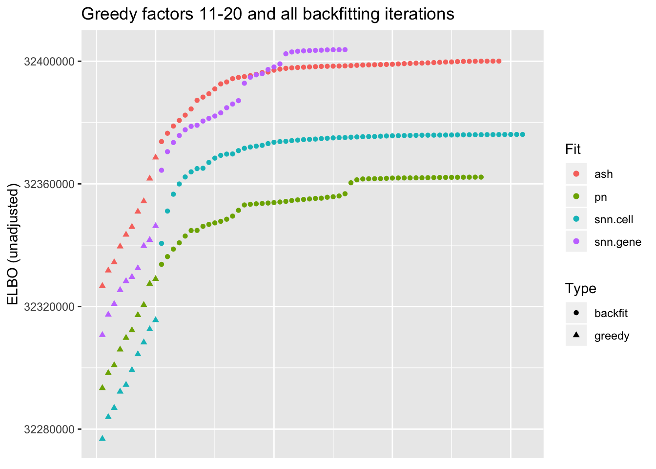
Results: Point-normal priors vs. scale mixtures of normals
I line up the point-normal and scale-mixture-of-normal factors so that similar factors are shown one on top of the other. Although many factors appear similar, the scale-mixture-of-normal fit looks much better to me: factor 6 does a better job at separating out dendritic cells, while factor 14 contains potentially useful information about CD19+ B cells.
pn.v.ash <- compare.factors(res$pn$fl, res$ash$fl)
plot.factors(res$pn, pbmc$cell.type, order(res$pn$fl$pve, decreasing = TRUE),
             title = "Point-normal priors")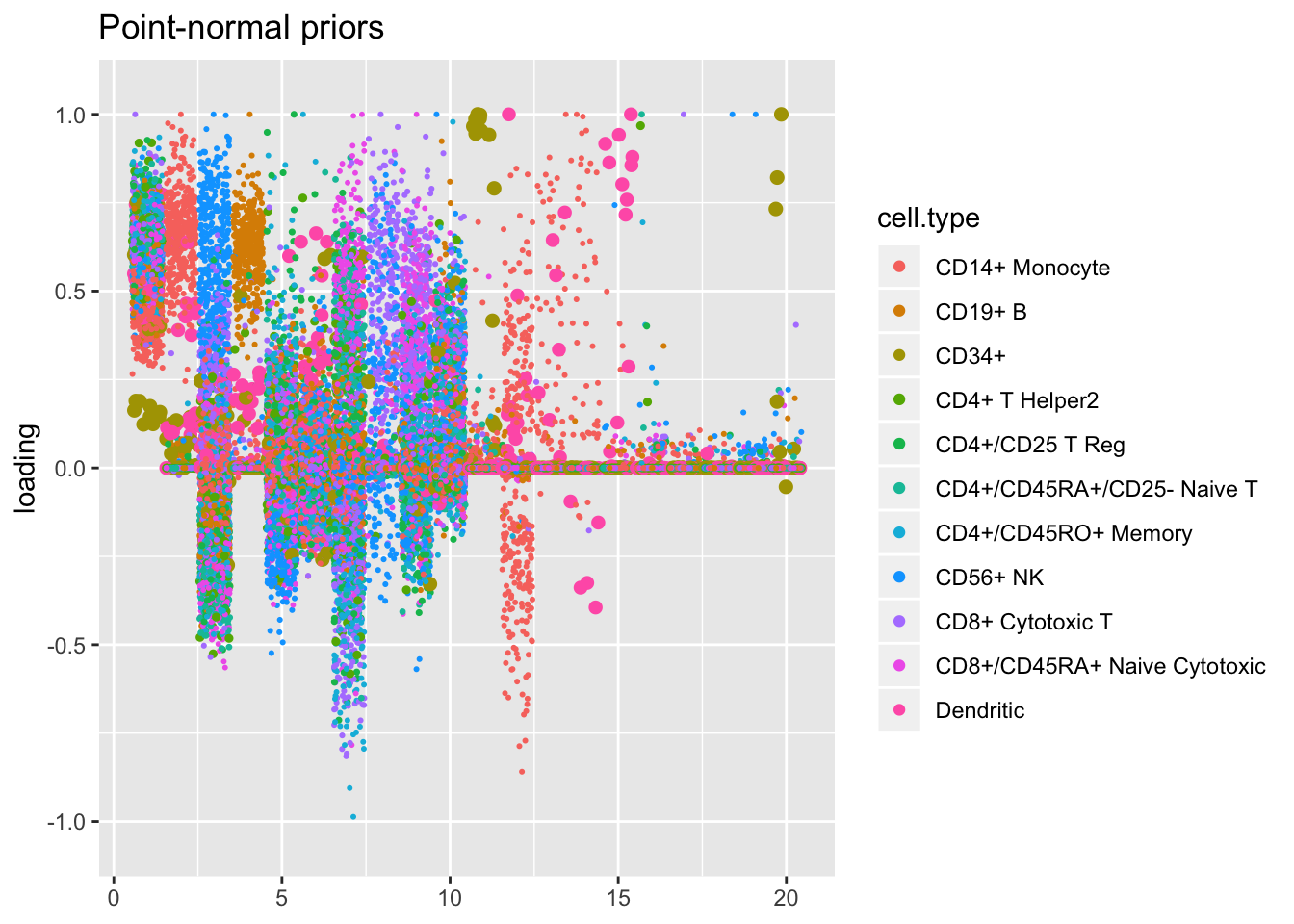
plot.factors(res$ash, pbmc$cell.type, pn.v.ash$fl2.k[order(res$pn$fl$pve, decreasing = TRUE)],
             title = "Scale mixtures of normals")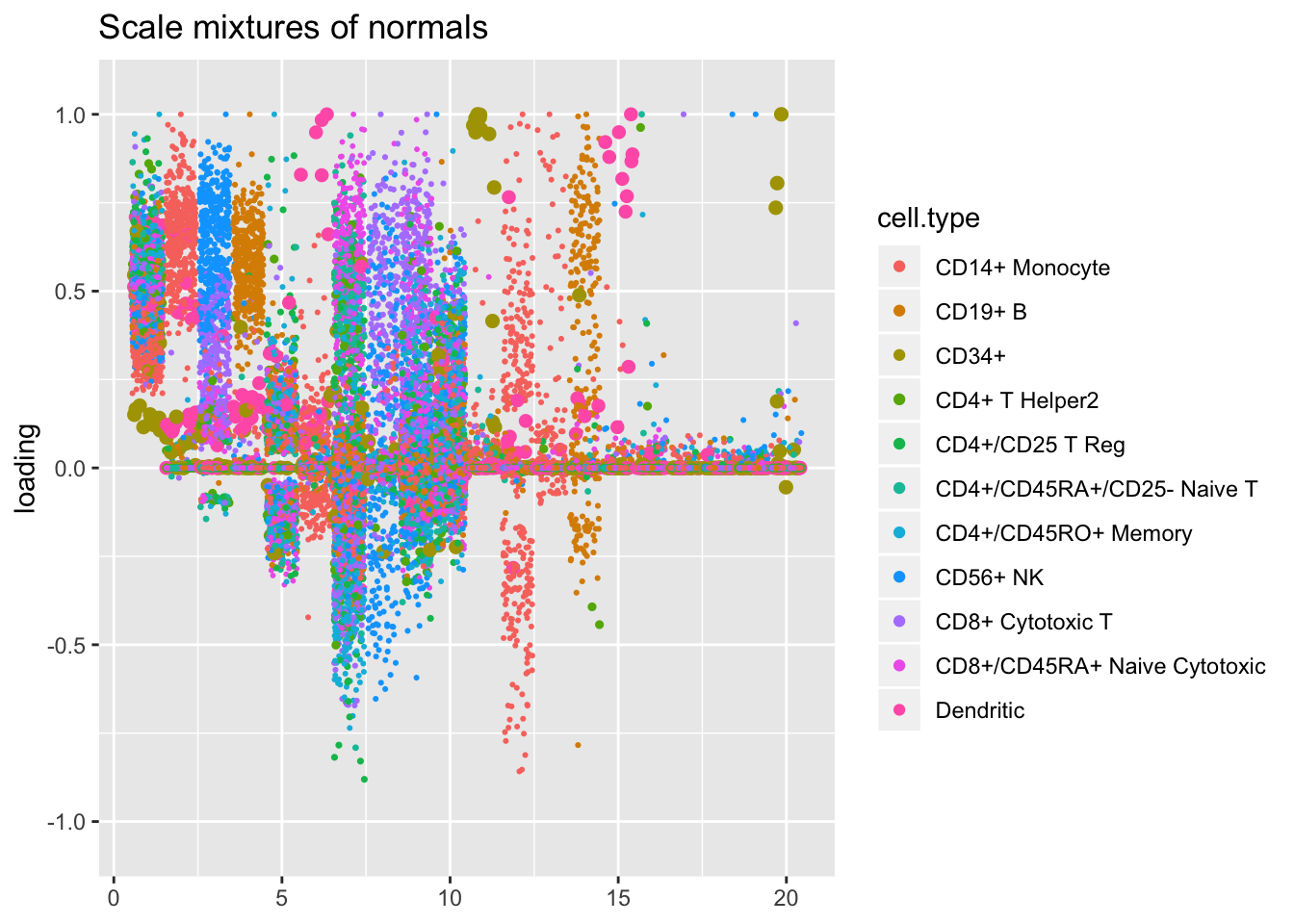
Results: Semi-nonnegative factorizations
For ease of comparison, I only consider the semi-nonnegative fit that puts nonnegative priors on gene loadings. As above, I line up similar factors. I denote a semi-nonnegative factor as “similar” to a point-normal factor if the gene loadings are strongly correlated (\(r \ge 0.7\)) with either the positive or the negative component of the point-normal gene loadings.
cor.thresh <- 0.7

pn.pos <- pmax(res$ash$fl$loadings.pm[[2]], 0)
pn.pos <- t(t(pn.pos) / apply(pn.pos, 2, function(x) sqrt(sum(x^2))))
pos.cor <- crossprod(res$snn.gene$fl$loadings.pm[[2]], pn.pos)

pn.neg <- -pmin(res$ash$fl$loadings.pm[[2]], 0)
pn.neg <- t(t(pn.neg) / apply(pn.neg, 2, function(x) sqrt(sum(x^2))))
pn.neg[, 1] <- 0
neg.cor <- crossprod(res$snn.gene$fl$loadings.pm[[2]], pn.neg)

is.cor <- (pmax(pos.cor, neg.cor) > cor.thresh)

pn.matched <- which(apply(is.cor, 2, any))
snn.matched <- unlist(lapply(pn.matched, function(x) which(is.cor[, x])))
# Duplicate factors where need be.
pn.matched <- rep(1:res$ash$fl$n.factors, times = apply(is.cor, 2, sum))

plot.factors(res$ash, pbmc$cell.type,
             pn.matched, title = "Point-normal (matched factors)")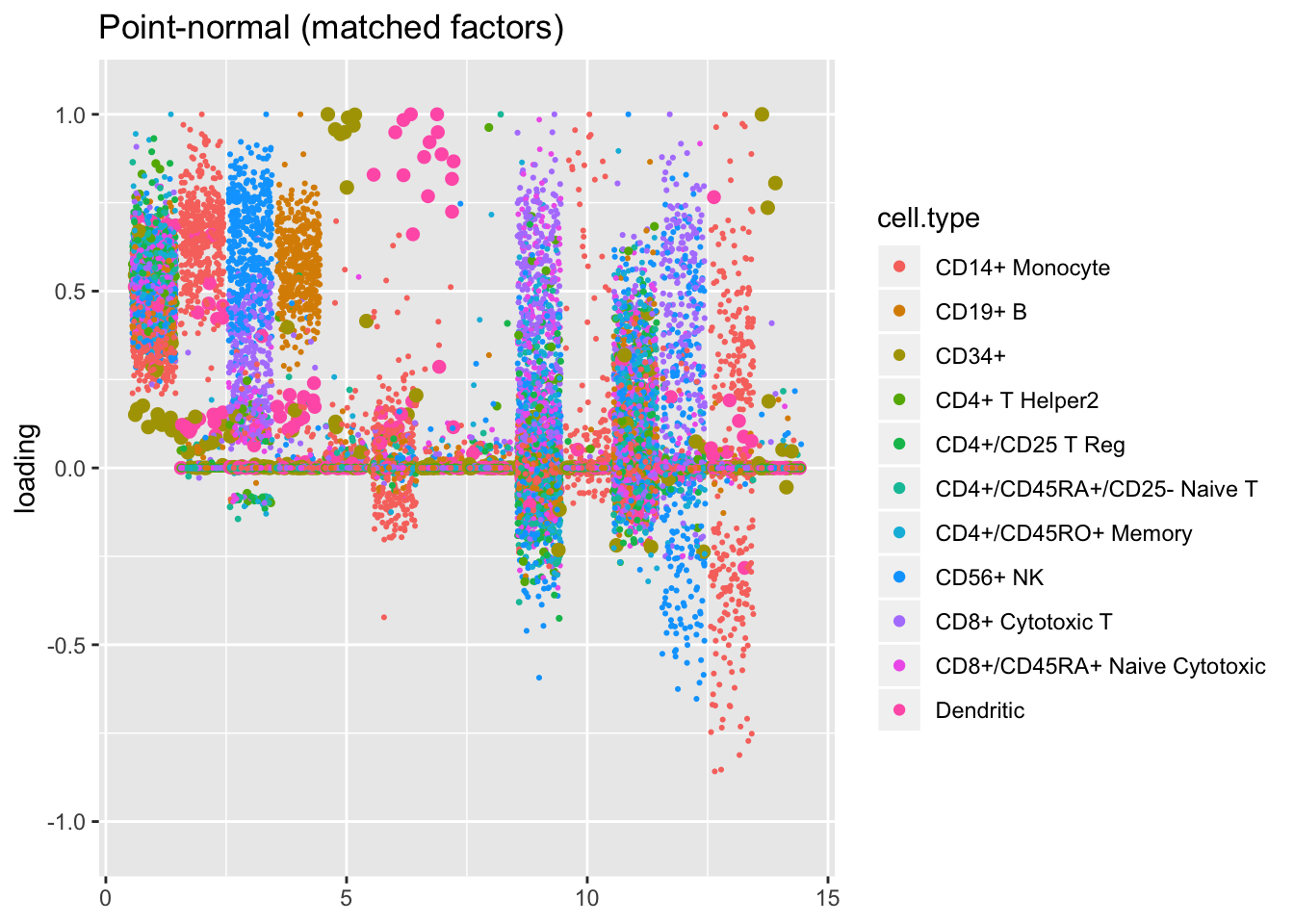
plot.factors(res$snn.gene, pbmc$cell.type,
             snn.matched, title = "Semi-nonnegative (matched factors)")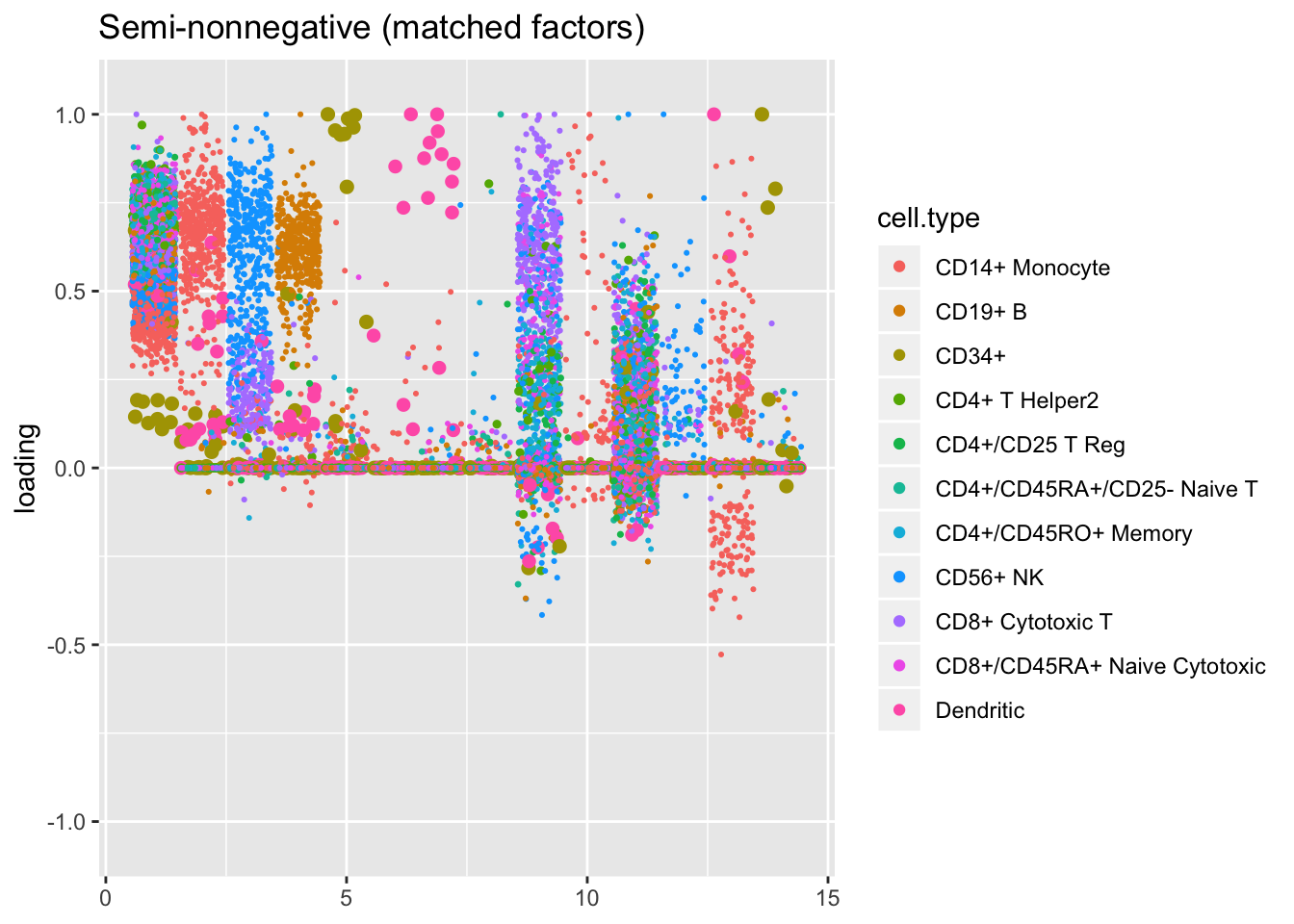
The remaining factors do not have counterparts.
snn.unmatched <- setdiff(1:res$snn.gene$fl$n.factors, snn.matched)
pn.unmatched <- setdiff(1:res$ash$fl$n.factors, pn.matched)

plot.factors(res$ash, pbmc$cell.type,
             pn.unmatched, title = "Point-normal (unmatched factors)")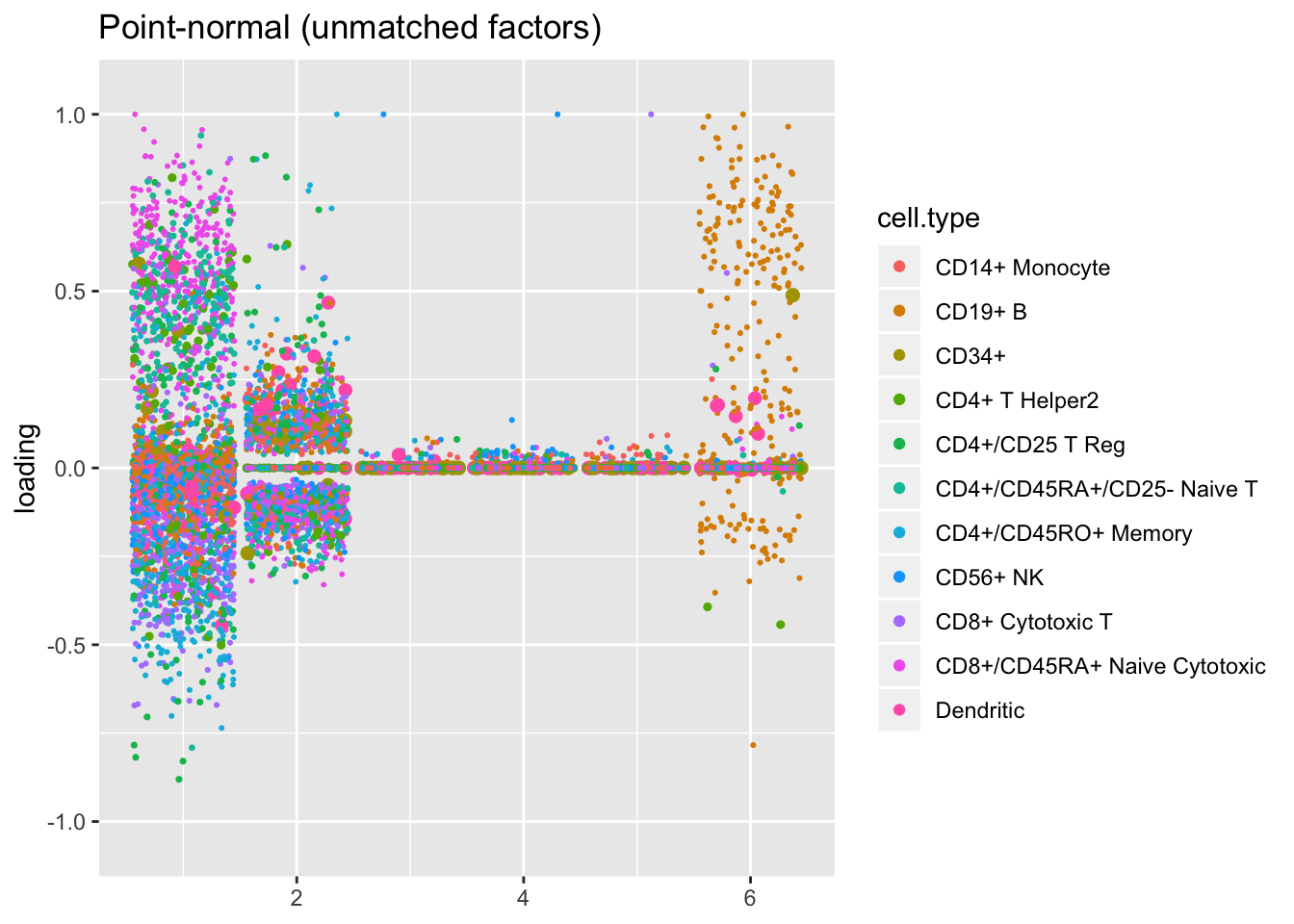
plot.factors(res$snn.gene, pbmc$cell.type,
             snn.unmatched, title = "Semi-nonnegative (unmatched factors)")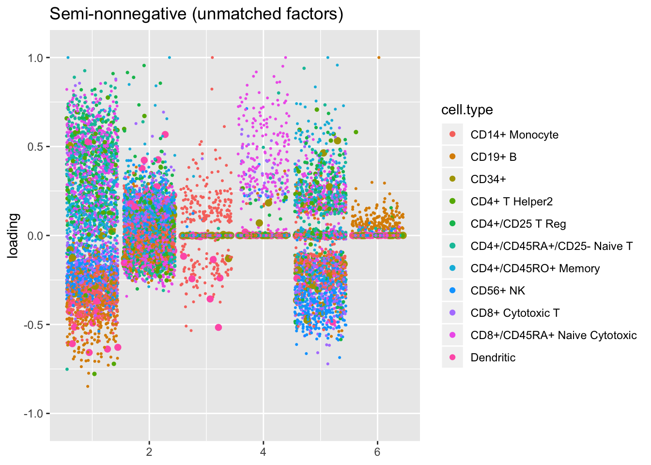
sessionInfo()R version 3.5.3 (2019-03-11)
Platform: x86_64-apple-darwin15.6.0 (64-bit)
Running under: macOS Mojave 10.14.6
Matrix products: default
BLAS: /Library/Frameworks/R.framework/Versions/3.5/Resources/lib/libRblas.0.dylib
LAPACK: /Library/Frameworks/R.framework/Versions/3.5/Resources/lib/libRlapack.dylib
locale:
[1] en_US.UTF-8/en_US.UTF-8/en_US.UTF-8/C/en_US.UTF-8/en_US.UTF-8
attached base packages:
[1] stats graphics grDevices utils datasets methods base
other attached packages:
[1] flashier_0.2.4 ggplot2_3.2.0 Matrix_1.2-15
loaded via a namespace (and not attached):
[1] Rcpp_1.0.1 plyr_1.8.4 highr_0.8
[4] compiler_3.5.3 pillar_1.3.1 git2r_0.25.2
[7] workflowr_1.2.0 iterators_1.0.10 tools_3.5.3
[10] digest_0.6.18 evaluate_0.13 tibble_2.1.1
[13] gtable_0.3.0 lattice_0.20-38 pkgconfig_2.0.2
[16] rlang_0.4.2 foreach_1.4.4 parallel_3.5.3
[19] yaml_2.2.0 ebnm_0.1-24 xfun_0.6
[22] withr_2.1.2 stringr_1.4.0 dplyr_0.8.0.1
[25] knitr_1.22 fs_1.2.7 rprojroot_1.3-2
[28] grid_3.5.3 tidyselect_0.2.5 glue_1.3.1
[31] R6_2.4.0 rmarkdown_1.12 mixsqp_0.3-31
[34] irlba_2.3.3 reshape2_1.4.3 ashr_2.2-38
[37] purrr_0.3.2 magrittr_1.5 whisker_0.3-2
[40] MASS_7.3-51.1 codetools_0.2-16 backports_1.1.3
[43] scales_1.0.0 htmltools_0.3.6 assertthat_0.2.1
[46] colorspace_1.4-1 labeling_0.3 stringi_1.4.3
[49] pscl_1.5.2 doParallel_1.0.14 lazyeval_0.2.2
[52] munsell_0.5.0 truncnorm_1.0-8 SQUAREM_2017.10-1
[55] crayon_1.3.4