Low-rank data representations
Jason Willwerscheid
9/21/2019
Last updated: 2019-09-21
Checks: 6 0
Knit directory: scFLASH/
This reproducible R Markdown analysis was created with workflowr (version 1.2.0). The Report tab describes the reproducibility checks that were applied when the results were created. The Past versions tab lists the development history.
Great! Since the R Markdown file has been committed to the Git repository, you know the exact version of the code that produced these results.
Great job! The global environment was empty. Objects defined in the global environment can affect the analysis in your R Markdown file in unknown ways. For reproduciblity it’s best to always run the code in an empty environment.
The command set.seed(20181103) was run prior to running the code in the R Markdown file. Setting a seed ensures that any results that rely on randomness, e.g. subsampling or permutations, are reproducible.
Great job! Recording the operating system, R version, and package versions is critical for reproducibility.
Nice! There were no cached chunks for this analysis, so you can be confident that you successfully produced the results during this run.
Great! You are using Git for version control. Tracking code development and connecting the code version to the results is critical for reproducibility. The version displayed above was the version of the Git repository at the time these results were generated.
Note that you need to be careful to ensure that all relevant files for the analysis have been committed to Git prior to generating the results (you can use wflow_publish or wflow_git_commit). workflowr only checks the R Markdown file, but you know if there are other scripts or data files that it depends on. Below is the status of the Git repository when the results were generated:
Ignored files:
    Ignored:    .DS_Store
    Ignored:    .Rhistory
    Ignored:    .Rproj.user/
    Ignored:    code/initialization/
    Ignored:    data/Ensembl2Reactome.txt
    Ignored:    data/droplet.rds
    Ignored:    data/mus_pathways.rds
    Ignored:    output/backfit/
    Ignored:    output/lowrank/
    Ignored:    output/prior_type/
    Ignored:    output/pseudocount/
    Ignored:    output/pseudocount_redux/
    Ignored:    output/size_factors/
    Ignored:    output/var_type/

Untracked files:
    Untracked:  analysis/NBapprox.Rmd
    Untracked:  analysis/deleted.Rmd
    Untracked:  analysis/trachea4.Rmd
    Untracked:  code/missing_data.R
    Untracked:  code/trachea4.R

Unstaged changes:
    Modified:   analysis/index.Rmd
    Modified:   analysis/pseudocount_redux.Rmd
Note that any generated files, e.g. HTML, png, CSS, etc., are not included in this status report because it is ok for generated content to have uncommitted changes.
These are the previous versions of the R Markdown and HTML files. If you’ve configured a remote Git repository (see ?wflow_git_remote), click on the hyperlinks in the table below to view them.
| File | Version | Author | Date | Message |
|---|---|---|---|---|
| Rmd | b8fb141 | Jason Willwerscheid | 2019-09-21 | wflow_publish(“analysis/lowrank.Rmd”) |
Introduction
If backfitting is performed, then fitting time will not be linear in the number of factors. Indeed, fitting 50 factors using scale-mixture-of-normal priors took me around 12 hours, while 30 factors took only 1.5 hours to converge at the same tolerance.
In an attempt to speed up the fitting process, I fit 50 factors using a low-rank representation of the data (a rank-100 SVD-like object obtained via rsvd) rather than the full data. The fitting time was indeed reduced (to around four hours), but the factors obtained were far inferior to the factors obtained using the full data (see below).
The failed experiment is instructive: in essence, it demonstrates that the top 50 flashier factors contain much different information from the information contained in the top 100 SVD factors. To give the low-rank strategy any chance of success, many more SVD factors would be needed — but this would defeat the point of using a low-rank data representation.
Note, for example, that the cost of multiplying a \(\left( U \in \mathbb{R}^{n \times k}, V \in \mathbb{R}^{p \times k} \right)\) low-rank representation against a \(n-\) or \(p-\)vector is \(k(n + p)\), while the cost of using the full data is \(snp\) (where \(s\) is the data sparsity). Thus, to have a chance of obtaining any speedup at all, it’s necessary that \[ k < s \min(n, p) \] In practice, though, \(k\) needs to be much smaller than this to produce a noticeable speedup. Indeed, the speedup obtained here (4 hours vs. 12 hours) was almost entirely due to the fact that fewer backfitting iterations were needed (160 vs. 413).
Factors
The code used to produce the fits can be viewed here.
source("./code/utils.R")
droplet <- readRDS("./data/droplet.rds")
droplet <- preprocess.droplet(droplet)

full.res <- list(fl = readRDS("./output/lowrank/full_fit50.rds"))
lr.res <- list(fl = readRDS("./output/lowrank/lowrank_fit50.rds"))
source("./code/utils.R")
plot.factors(full.res, droplet$cell.type, 1:25, title = "Full data, factors 1-25")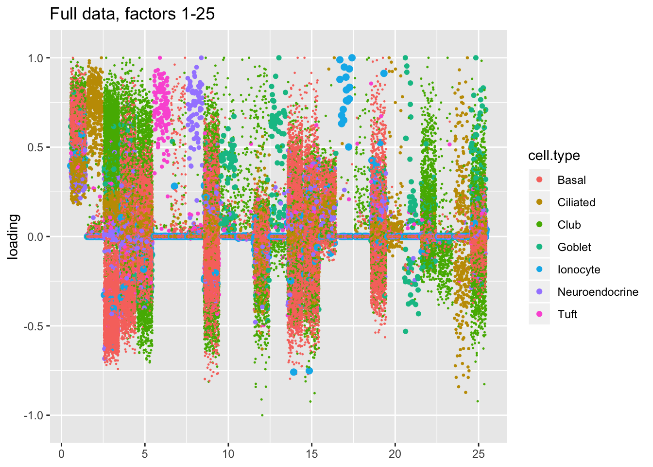
plot.factors(full.res, droplet$cell.type, 26:50, title = "Full data, factors 26-50")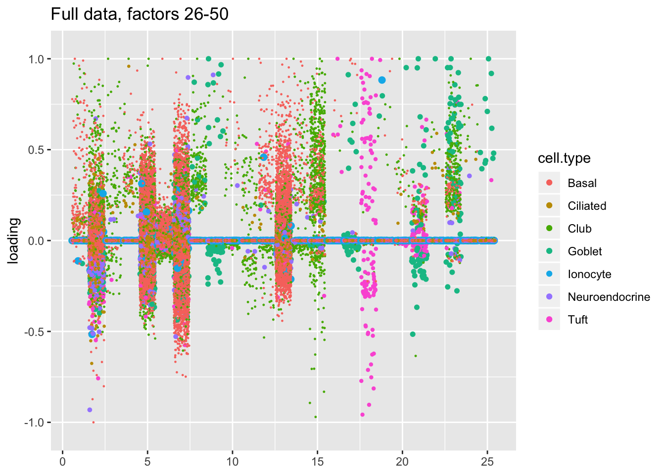
plot.factors(lr.res, droplet$cell.type, 1:25, title = "Low-rank data, factors 1-25")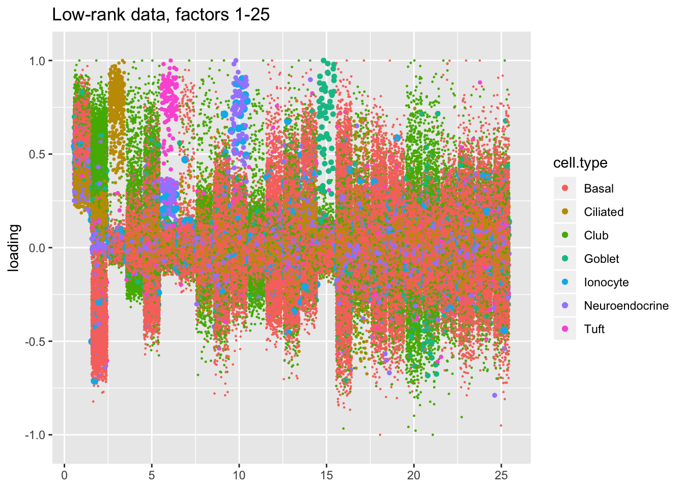
plot.factors(lr.res, droplet$cell.type, 26:50, title = "Low-rank data, factors 26-50")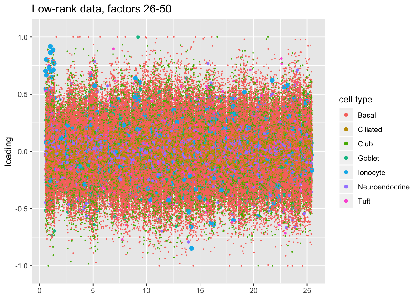
sessionInfo()R version 3.5.3 (2019-03-11)
Platform: x86_64-apple-darwin15.6.0 (64-bit)
Running under: macOS Mojave 10.14.6
Matrix products: default
BLAS: /Library/Frameworks/R.framework/Versions/3.5/Resources/lib/libRblas.0.dylib
LAPACK: /Library/Frameworks/R.framework/Versions/3.5/Resources/lib/libRlapack.dylib
locale:
[1] en_US.UTF-8/en_US.UTF-8/en_US.UTF-8/C/en_US.UTF-8/en_US.UTF-8
attached base packages:
[1] stats graphics grDevices utils datasets methods base
other attached packages:
[1] flashier_0.1.17 ggplot2_3.2.0 Matrix_1.2-15
loaded via a namespace (and not attached):
[1] Rcpp_1.0.1 plyr_1.8.4 compiler_3.5.3
[4] pillar_1.3.1 git2r_0.25.2 workflowr_1.2.0
[7] iterators_1.0.10 tools_3.5.3 digest_0.6.18
[10] evaluate_0.13 tibble_2.1.1 gtable_0.3.0
[13] lattice_0.20-38 pkgconfig_2.0.2 rlang_0.3.1
[16] foreach_1.4.4 parallel_3.5.3 yaml_2.2.0
[19] ebnm_0.1-24 xfun_0.6 withr_2.1.2
[22] stringr_1.4.0 dplyr_0.8.0.1 knitr_1.22
[25] fs_1.2.7 rprojroot_1.3-2 grid_3.5.3
[28] tidyselect_0.2.5 glue_1.3.1 R6_2.4.0
[31] rmarkdown_1.12 mixsqp_0.1-119 reshape2_1.4.3
[34] ashr_2.2-38 purrr_0.3.2 magrittr_1.5
[37] whisker_0.3-2 MASS_7.3-51.1 codetools_0.2-16
[40] backports_1.1.3 scales_1.0.0 htmltools_0.3.6
[43] assertthat_0.2.1 colorspace_1.4-1 labeling_0.3
[46] stringi_1.4.3 pscl_1.5.2 doParallel_1.0.14
[49] lazyeval_0.2.2 munsell_0.5.0 truncnorm_1.0-8
[52] SQUAREM_2017.10-1 crayon_1.3.4