Montoro et al. droplet dataset
Jason Willwerscheid
8/12/2019
Last updated: 2019-08-12
Checks: 6 0
Knit directory: scFLASH/
This reproducible R Markdown analysis was created with workflowr (version 1.2.0). The Report tab describes the reproducibility checks that were applied when the results were created. The Past versions tab lists the development history.
Great! Since the R Markdown file has been committed to the Git repository, you know the exact version of the code that produced these results.
Great job! The global environment was empty. Objects defined in the global environment can affect the analysis in your R Markdown file in unknown ways. For reproduciblity it’s best to always run the code in an empty environment.
The command set.seed(20181103) was run prior to running the code in the R Markdown file. Setting a seed ensures that any results that rely on randomness, e.g. subsampling or permutations, are reproducible.
Great job! Recording the operating system, R version, and package versions is critical for reproducibility.
Nice! There were no cached chunks for this analysis, so you can be confident that you successfully produced the results during this run.
Great! You are using Git for version control. Tracking code development and connecting the code version to the results is critical for reproducibility. The version displayed above was the version of the Git repository at the time these results were generated.
Note that you need to be careful to ensure that all relevant files for the analysis have been committed to Git prior to generating the results (you can use wflow_publish or wflow_git_commit). workflowr only checks the R Markdown file, but you know if there are other scripts or data files that it depends on. Below is the status of the Git repository when the results were generated:
Ignored files:
    Ignored:    .DS_Store
    Ignored:    .Rhistory
    Ignored:    .Rproj.user/

Untracked files:
    Untracked:  analysis/NBapprox.Rmd
    Untracked:  analysis/pseudocount2.Rmd
    Untracked:  analysis/trachea4.Rmd
    Untracked:  code/missing_data.R
    Untracked:  code/pseudocounts.R
    Untracked:  code/trachea4.R
    Untracked:  code/var_type.R
    Untracked:  data/Ensembl2Reactome.txt
    Untracked:  data/droplet.rds
    Untracked:  data/hard_bimodal1.txt
    Untracked:  data/hard_bimodal2.txt
    Untracked:  data/hard_bimodal3.txt
    Untracked:  data/mus_pathways.rds
    Untracked:  docs/figure/pseudocount2.Rmd/
    Untracked:  output/pseudocount/

Unstaged changes:
    Modified:   analysis/pseudocount.Rmd
    Modified:   code/sc_comparisons.R
    Modified:   code/utils.R
Note that any generated files, e.g. HTML, png, CSS, etc., are not included in this status report because it is ok for generated content to have uncommitted changes.
These are the previous versions of the R Markdown and HTML files. If you’ve configured a remote Git repository (see ?wflow_git_remote), click on the hyperlinks in the table below to view them.
| File | Version | Author | Date | Message |
|---|---|---|---|---|
| Rmd | cbc50e1 | Jason Willwerscheid | 2019-08-12 | wflow_publish(“analysis/droplet.Rmd”) |
droplet <- readRDS("./data/droplet.rds")
source("./code/utils.R")
The droplet-based 3’ scRNA-seq dataset analyzed in Montoro et al. (2018) can be obtained here. It includes counts for 18,388 genes and 7,193 cells. Only 9.3% of all counts are nonzero. The data takes up 143 MB when loaded into memory as a sparse Matrix object.
The original analysis assigns each cell to one of seven cell types. The cells are also labelled according to the mice they come from.
cell.type <- as.factor(sapply(strsplit(colnames(droplet), "_"), `[`, 3))
plot.category(cell.type, title = "Number of Cells per Cell Type")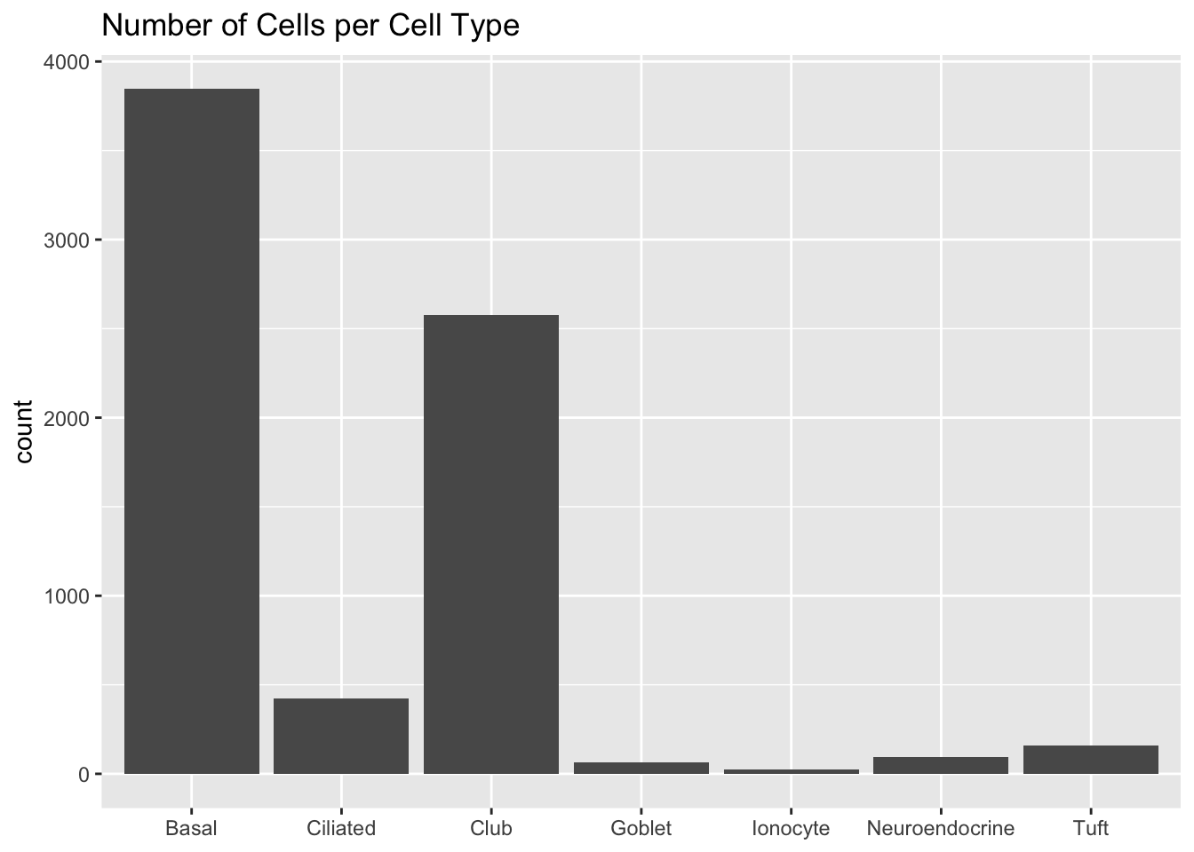
mouse <- as.factor(sapply(strsplit(colnames(droplet), "_"), `[`, 1))
plot.category(mouse, title = "Number of Cells per Mouse")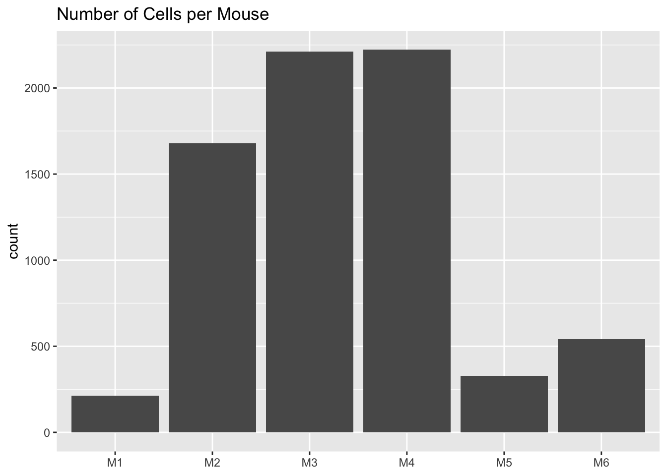
Library size is distributed as follows.
plot.libsize(droplet)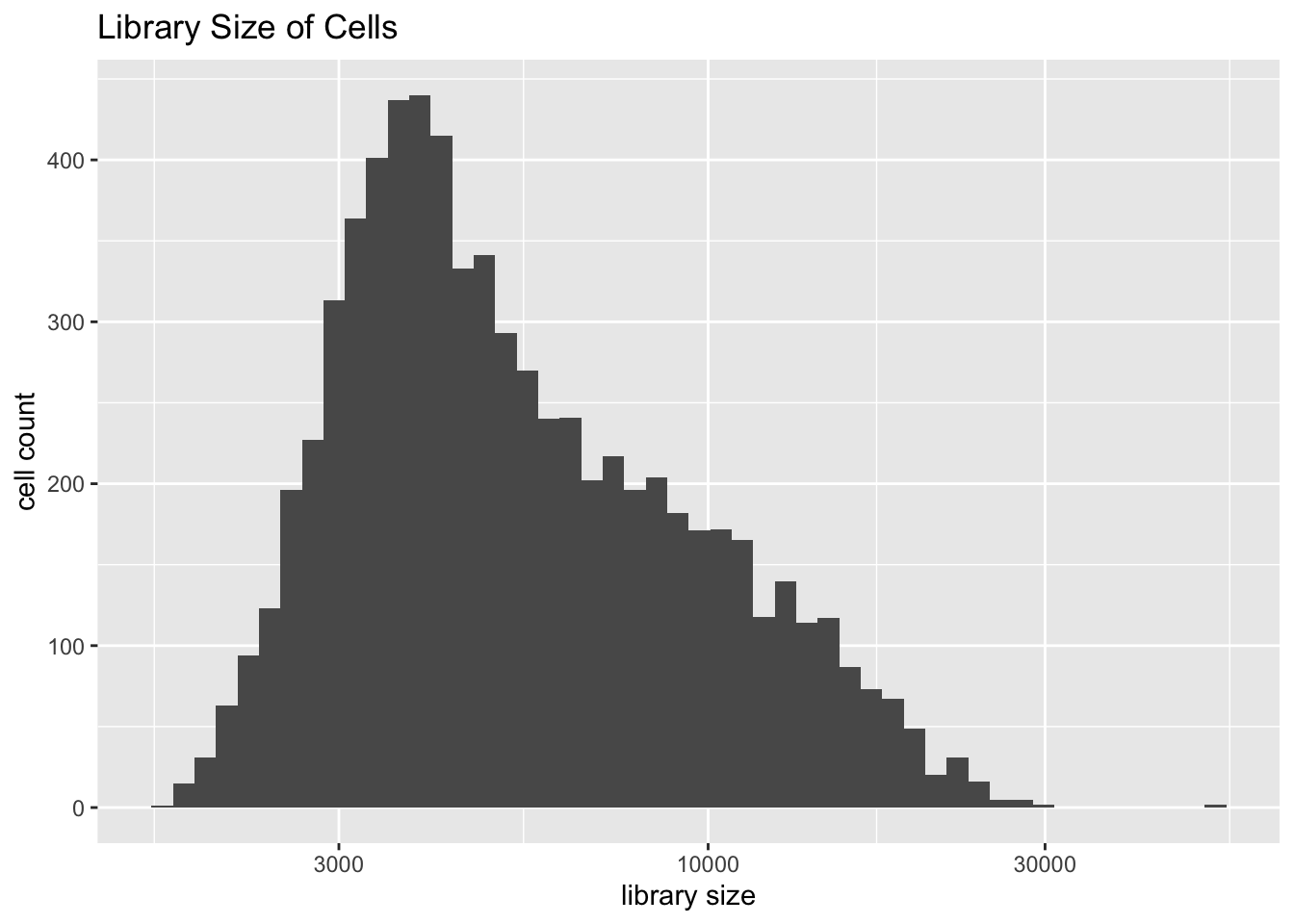
Note the presence of extreme outliers. There are two of them, and both turn out to be goblet cells. I think that they should be removed from the dataset before analysis.
table(cell.type[which(colSums(droplet) > 30000)])#>
#> Basal Ciliated Club Goblet Ionocyte
#> 0 0 0 2 0
#> Neuroendocrine Tuft
#> 0 0Mean expression is distributed as follows.
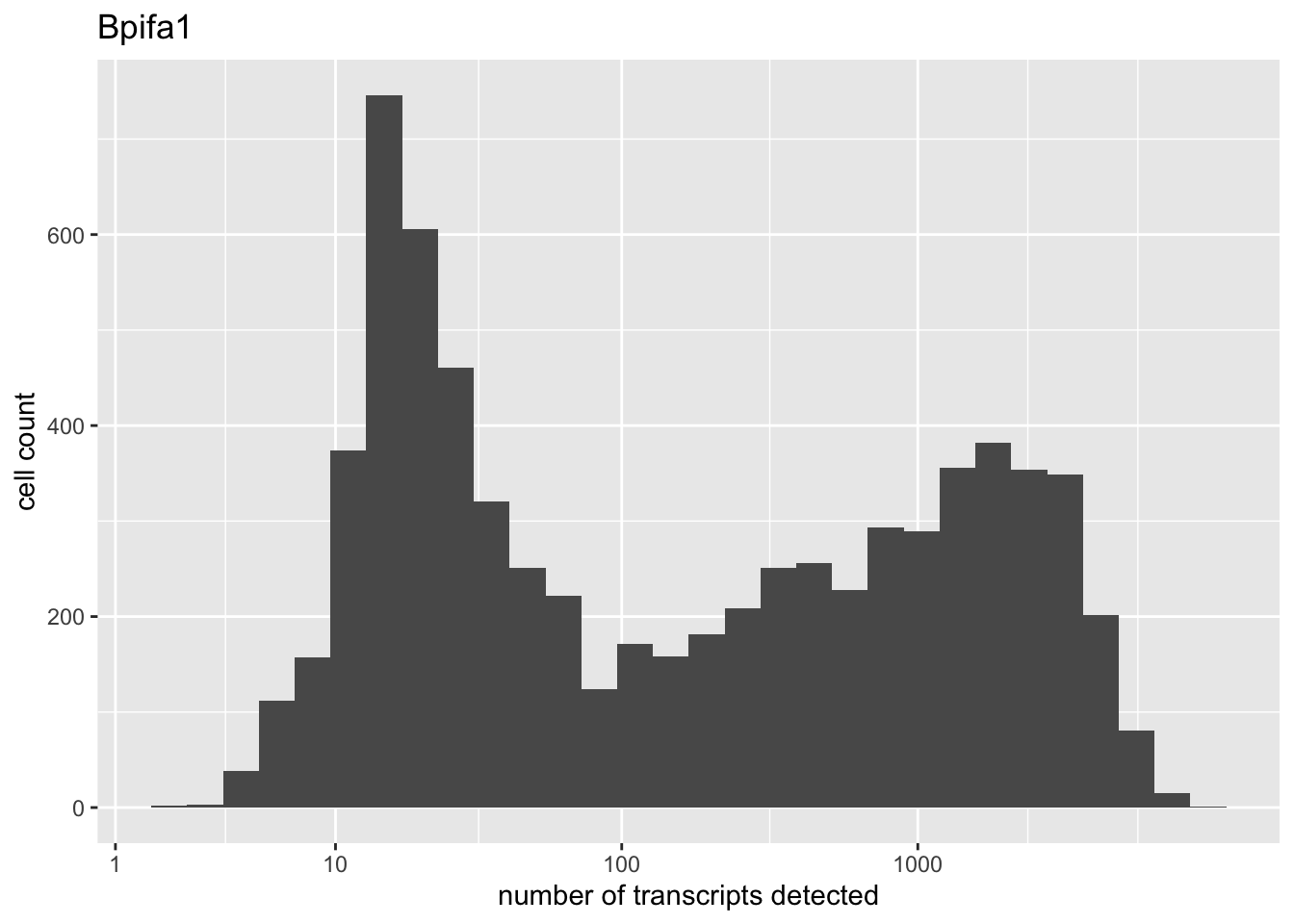
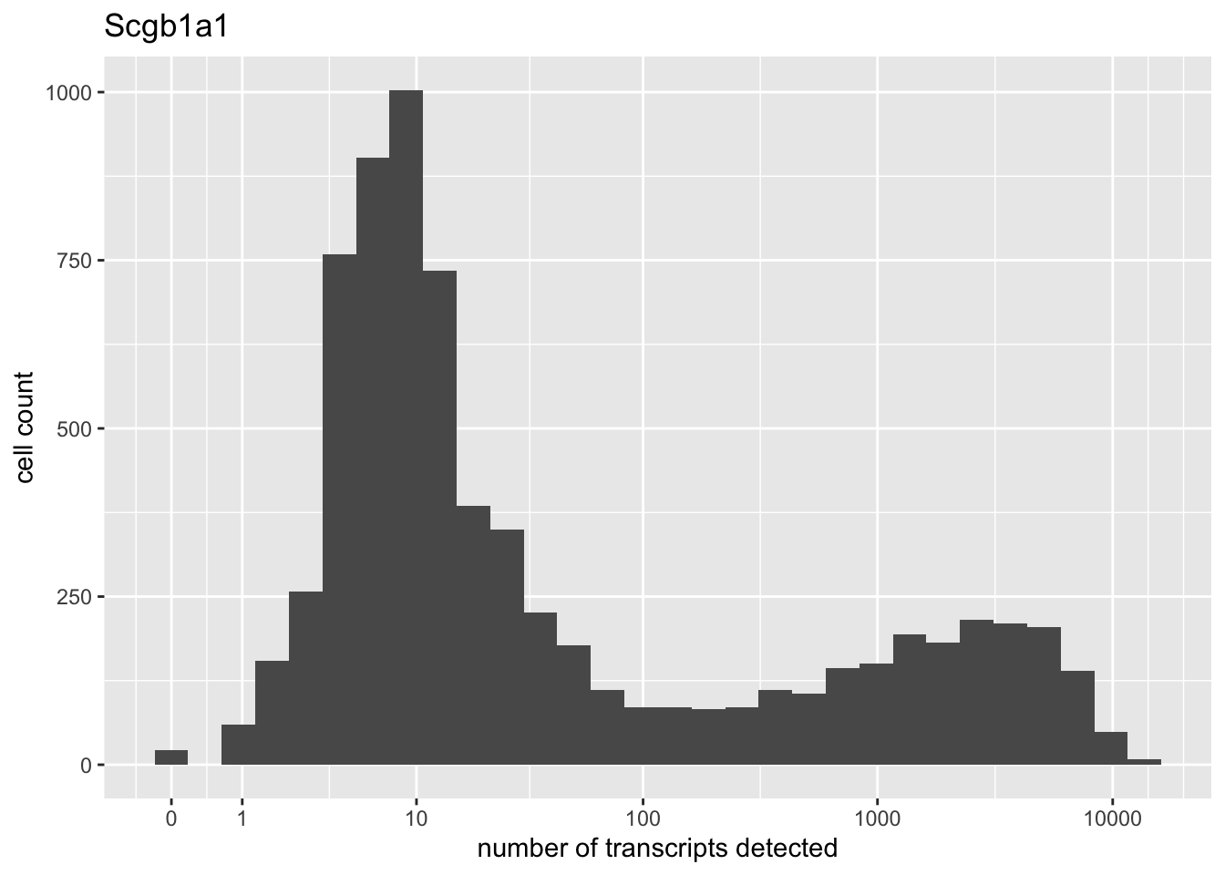
plot.meanexp(droplet)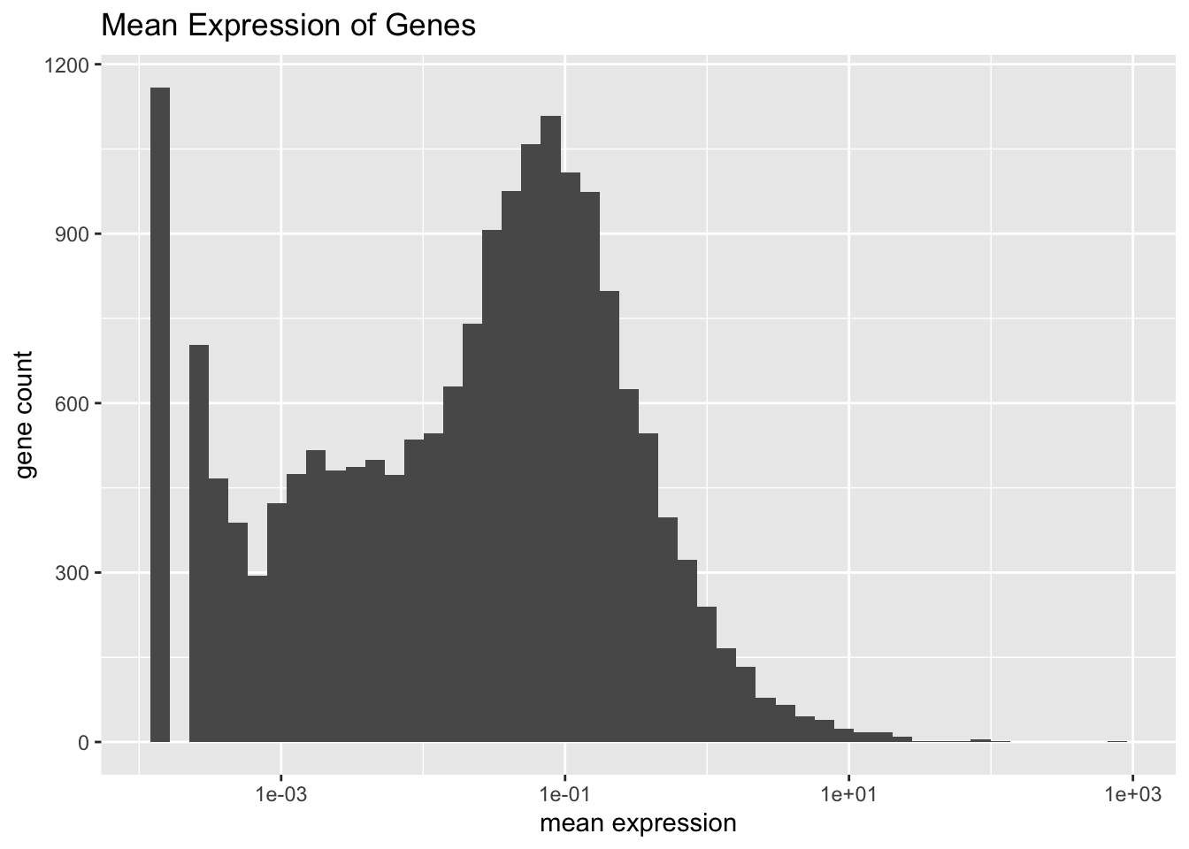
There are two genes that are on average much more highly expressed than any other gene: Bpifa1 and Scgb1a1. Both have bimodal distributions.
high.exp <- names(which(rowMeans(droplet) > 200))
for (gene in high.exp) {
  plot(plot.gene(droplet, gene))
}
sessionInfo()#> R version 3.5.3 (2019-03-11)
#> Platform: x86_64-apple-darwin15.6.0 (64-bit)
#> Running under: macOS Mojave 10.14.6
#>
#> Matrix products: default
#> BLAS: /Library/Frameworks/R.framework/Versions/3.5/Resources/lib/libRblas.0.dylib
#> LAPACK: /Library/Frameworks/R.framework/Versions/3.5/Resources/lib/libRlapack.dylib
#>
#> locale:
#> [1] en_US.UTF-8/en_US.UTF-8/en_US.UTF-8/C/en_US.UTF-8/en_US.UTF-8
#>
#> attached base packages:
#> [1] stats graphics grDevices utils datasets methods base
#>
#> other attached packages:
#> [1] ggplot2_3.2.0 Matrix_1.2-15
#>
#> loaded via a namespace (and not attached):
#> [1] Rcpp_1.0.1 compiler_3.5.3 pillar_1.3.1 git2r_0.25.2
#> [5] workflowr_1.2.0 tools_3.5.3 digest_0.6.18 evaluate_0.13
#> [9] tibble_2.1.1 gtable_0.3.0 lattice_0.20-38 pkgconfig_2.0.2
#> [13] rlang_0.3.1 yaml_2.2.0 xfun_0.6 withr_2.1.2
#> [17] stringr_1.4.0 dplyr_0.8.0.1 knitr_1.22 fs_1.2.7
#> [21] rprojroot_1.3-2 grid_3.5.3 tidyselect_0.2.5 glue_1.3.1
#> [25] R6_2.4.0 rmarkdown_1.12 purrr_0.3.2 magrittr_1.5
#> [29] whisker_0.3-2 backports_1.1.3 scales_1.0.0 htmltools_0.3.6
#> [33] assertthat_0.2.1 colorspace_1.4-1 labeling_0.3 stringi_1.4.3
#> [37] lazyeval_0.2.2 munsell_0.5.0 crayon_1.3.4