Variance Regularization: Part One
Jason Willwerscheid
3/10/2020
Last updated: 2020-03-11
Checks: 6 0
Knit directory: scFLASH/
This reproducible R Markdown analysis was created with workflowr (version 1.2.0). The Report tab describes the reproducibility checks that were applied when the results were created. The Past versions tab lists the development history.
Great! Since the R Markdown file has been committed to the Git repository, you know the exact version of the code that produced these results.
Great job! The global environment was empty. Objects defined in the global environment can affect the analysis in your R Markdown file in unknown ways. For reproduciblity it’s best to always run the code in an empty environment.
The command set.seed(20181103) was run prior to running the code in the R Markdown file. Setting a seed ensures that any results that rely on randomness, e.g. subsampling or permutations, are reproducible.
Great job! Recording the operating system, R version, and package versions is critical for reproducibility.
Nice! There were no cached chunks for this analysis, so you can be confident that you successfully produced the results during this run.
Great! You are using Git for version control. Tracking code development and connecting the code version to the results is critical for reproducibility. The version displayed above was the version of the Git repository at the time these results were generated.
Note that you need to be careful to ensure that all relevant files for the analysis have been committed to Git prior to generating the results (you can use wflow_publish or wflow_git_commit). workflowr only checks the R Markdown file, but you know if there are other scripts or data files that it depends on. Below is the status of the Git repository when the results were generated:
Ignored files:
    Ignored:    .DS_Store
    Ignored:    .Rhistory
    Ignored:    .Rproj.user/
    Ignored:    code/initialization/
    Ignored:    data-raw/10x_assigned_cell_types.R
    Ignored:    data/.DS_Store
    Ignored:    data/10x/
    Ignored:    data/Ensembl2Reactome.txt
    Ignored:    data/droplet.rds
    Ignored:    data/mus_pathways.rds
    Ignored:    output/backfit/
    Ignored:    output/final_montoro/
    Ignored:    output/lowrank/
    Ignored:    output/prior_type/
    Ignored:    output/pseudocount/
    Ignored:    output/pseudocount_redux/
    Ignored:    output/size_factors/
    Ignored:    output/var_type/

Untracked files:
    Untracked:  analysis/NBapprox.Rmd
    Untracked:  analysis/trachea4.Rmd
    Untracked:  code/alt_montoro/
    Untracked:  code/missing_data.R
    Untracked:  code/pulseseq/
    Untracked:  code/trachea4.R
    Untracked:  code/var_reg/
    Untracked:  fl_tmp.rds
    Untracked:  output/alt_montoro/
    Untracked:  output/pulseseq_fit.rds
    Untracked:  output/var_reg/

Unstaged changes:
    Modified:   code/utils.R
    Modified:   data-raw/pbmc.R
Note that any generated files, e.g. HTML, png, CSS, etc., are not included in this status report because it is ok for generated content to have uncommitted changes.
These are the previous versions of the R Markdown and HTML files. If you’ve configured a remote Git repository (see ?wflow_git_remote), click on the hyperlinks in the table below to view them.
| File | Version | Author | Date | Message |
|---|---|---|---|---|
| Rmd | 3af14c0 | Jason Willwerscheid | 2020-03-11 | wflow_publish(“analysis/var_reg_pbmc.Rmd”) |
Introduction
Although I prefer a gene-wise variance structure, it can cause problems for backfits. When the low-rank EBMF structure very closely approximates the observed expression for a particular gene, then the estimated residual variance for that gene can blow up to infinity. This typically happens with very sparsely expressed genes, so removing genes with zero counts in a large majority of cells mitigates the problem. I don’t want to remove too many genes, however, since sparsely expressed genes can provide important information about rare cell types (e.g., Cftr and ionocytes).
Up until now, I’ve dealt with this problem is a very ad hoc manner: I set the minimum gene-wise residual variance obtained from the greedy fit as the minimum for all residual variances estimated during the backfit. Here I explore a less ad-hoc approach in which I put a prior on the gene-wise precisions:
\[ 1 / \sigma_j^2 \sim \text{Exponential}(\lambda) \]
The \(\sigma_j\)s can then be estimated by solving an empirical Bayes Poisson means (EBPM) problem. The ebpm package is not yet able to solve this particular EBPM problem, so in this analysis I’ll fix \(\lambda\) and explore results for various choices. (I attempted to use exponential_mixture and point_gamma prior families, but they did a very poor job at regularizing the variance estimates.)
All fits “pre-scale” cells, add 20 factors greedily using point-normal priors, and then backfit. The code used to produce the fits can be viewed here.
suppressMessages(library(tidyverse))
suppressMessages(library(Matrix))

source("./code/utils.R")
pbmc <- readRDS("./data/10x/pbmc.rds")
pbmc <- preprocess.pbmc(pbmc)

res <- readRDS("./output/var_reg/varreg_fits.rds")
Results: ELBO
As the scale of the prior increases, less shrinkage will be applied, so that estimates will be closer to the MLE estimates and a larger ELBO will result. Interestingly, the same is not true for the likelihood of the implied discrete distribution, which peaks somewhere around \(\lambda = 100\) or \(\lambda = 1000\).
This order of magnitude for \(\lambda\) makes intuitive sense. I’ve retained genes that have nonzero counts in at least 10 of the 3206 cells. If we regard the true marginal distribution for gene \(j\) as \(\text{Poisson}(\nu)\), then (using the ML estimate for \(\nu\)) its residual variance will be at least \(10 / 3206\). (One can also show that if the true distribution is a mixture \(\pi_1 \text{Poisson}(\nu_1) + \pi_2 \text{Poisson}(\nu_2)\), then the variance is bounded below by \(\mu(1 - \mu)\), where \(\mu\) is the mean of the distribution: \(\mu = \pi_1 \nu_1 + \pi_2 \nu_2\). Plugging in \(\hat{\mu} = 10/3206\) gives an upper bound of 321.6 for gene-wise precisions.)
prior.scale <- 10^(0:5)
elbo.df <- tibble(scale = prior.scale,
                  elbo = sapply(res, function(x) x$fl$elbo),
                  llik = sapply(res, function(x) x$p.vals$llik))

ggplot(elbo.df, aes(x = scale, y = elbo)) +
  geom_point() +
  scale_x_log10() +
  labs(x = "Scale of prior",
       y = NULL,
       title = "ELBO")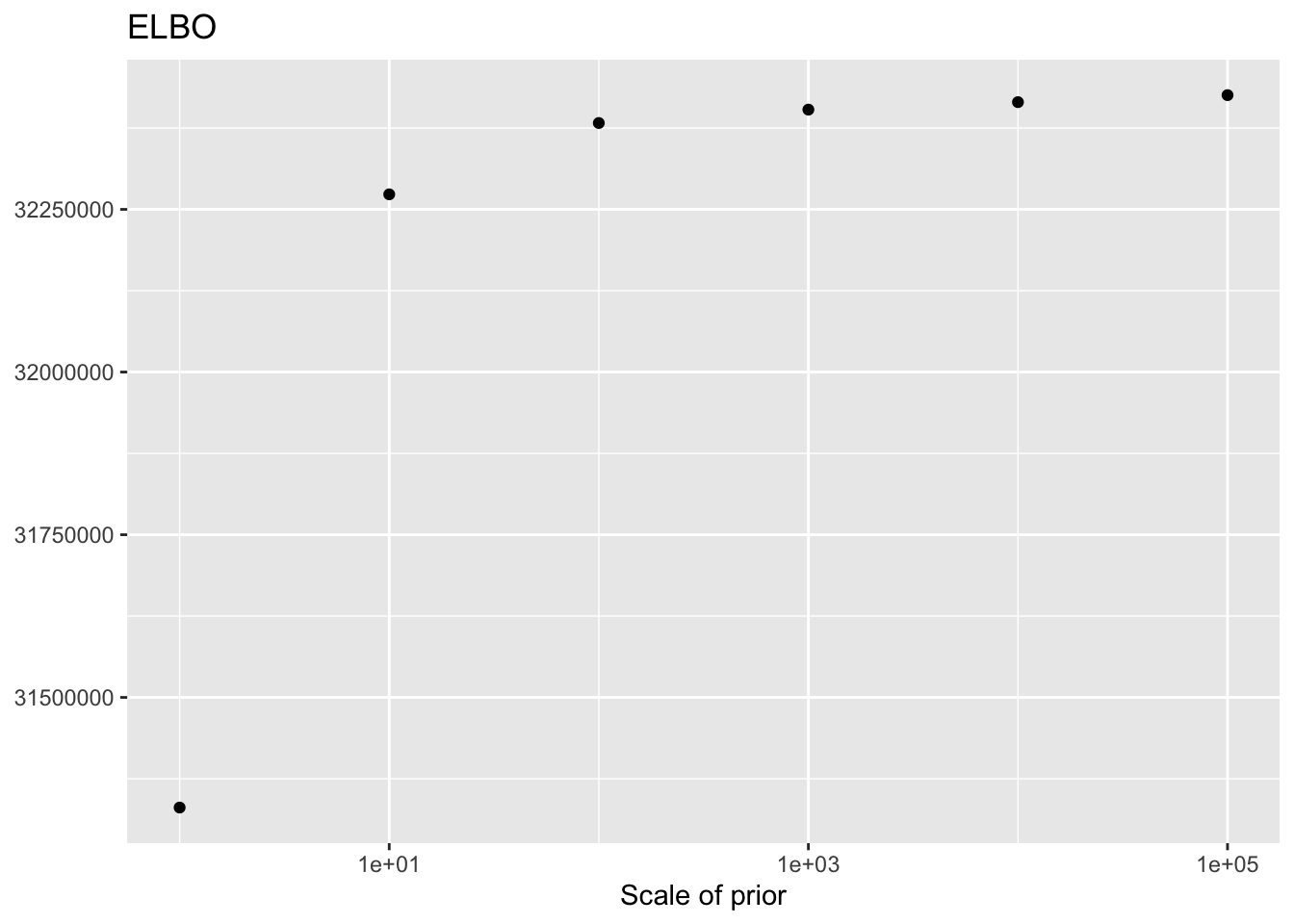
ggplot(elbo.df, aes(x = scale, y = llik)) +
  geom_point() +
  scale_x_log10() +
  labs(x = "Scale of prior",
       y = NULL,
       title = "Likelihood of implied discrete distribution")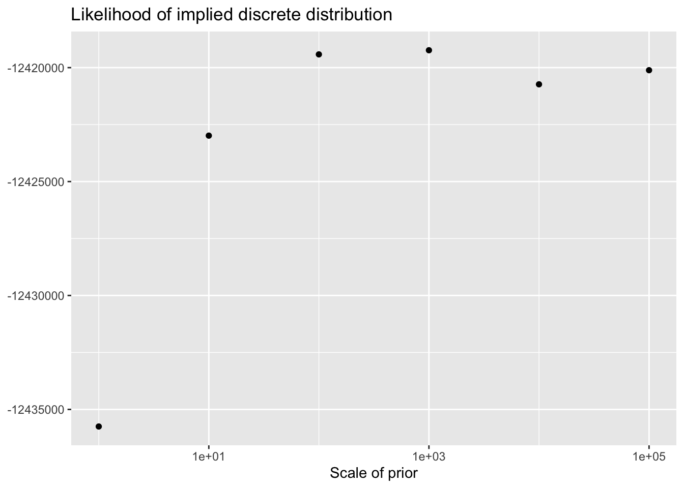
Results: Factor comparisons
Plotted factors look fairly similar for all choices of \(\lambda\), especially for more reasonable choices (\(\lambda > 100\)).
plot.factors(res$scale1, pbmc$cell.type, kset = order(res$scale1$fl$pve, decreasing = TRUE),
             title = "Scale = 1")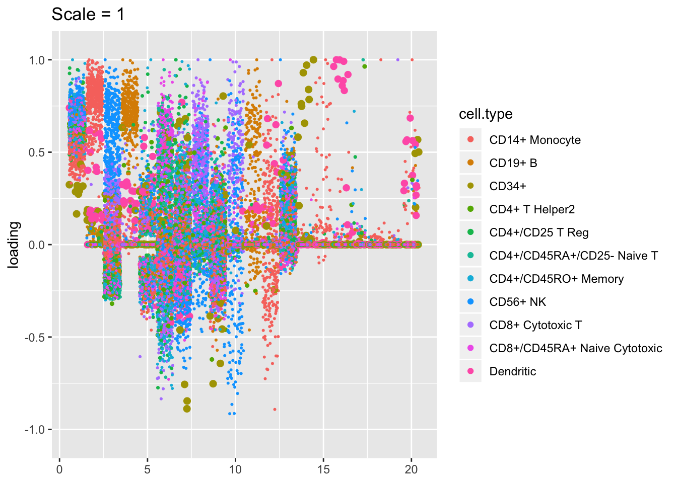
plot.factors(res$scale100, pbmc$cell.type, kset = order(res$scale100$fl$pve, decreasing = TRUE),
             title = "Scale = 100")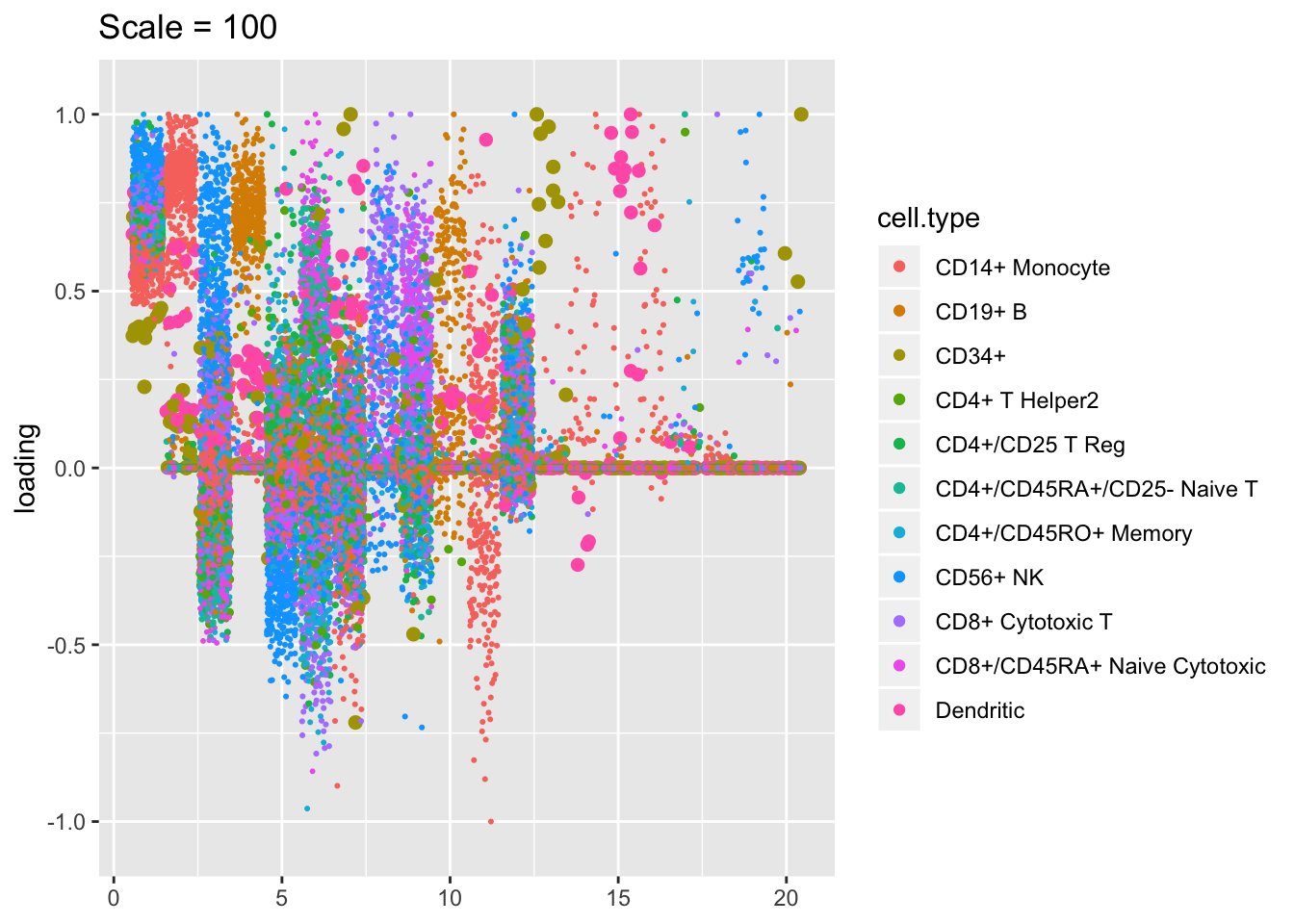
plot.factors(res$scale10000, pbmc$cell.type, kset = order(res$scale10000$fl$pve, decreasing = TRUE),
             title = "Scale = 10000")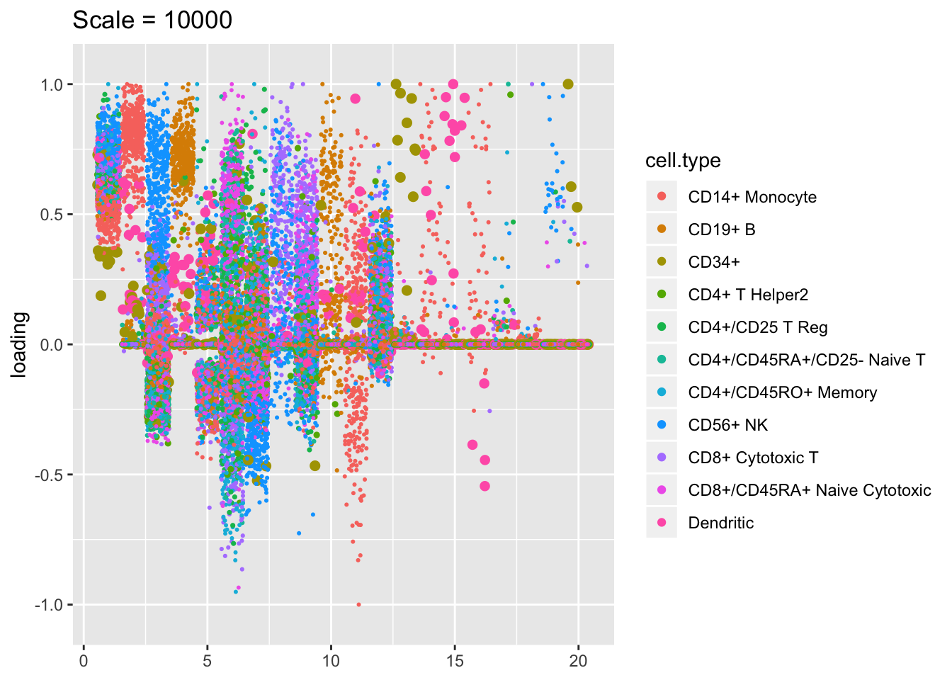
sessionInfo()R version 3.5.3 (2019-03-11)
Platform: x86_64-apple-darwin15.6.0 (64-bit)
Running under: macOS Mojave 10.14.6
Matrix products: default
BLAS: /Library/Frameworks/R.framework/Versions/3.5/Resources/lib/libRblas.0.dylib
LAPACK: /Library/Frameworks/R.framework/Versions/3.5/Resources/lib/libRlapack.dylib
locale:
[1] en_US.UTF-8/en_US.UTF-8/en_US.UTF-8/C/en_US.UTF-8/en_US.UTF-8
attached base packages:
[1] stats graphics grDevices utils datasets methods base
other attached packages:
[1] flashier_0.2.4 Matrix_1.2-15 forcats_0.4.0 stringr_1.4.0
[5] dplyr_0.8.0.1 purrr_0.3.2 readr_1.3.1 tidyr_0.8.3
[9] tibble_2.1.1 ggplot2_3.2.0 tidyverse_1.2.1
loaded via a namespace (and not attached):
[1] Rcpp_1.0.1 lubridate_1.7.4 lattice_0.20-38
[4] assertthat_0.2.1 rprojroot_1.3-2 digest_0.6.18
[7] foreach_1.4.4 truncnorm_1.0-8 R6_2.4.0
[10] cellranger_1.1.0 plyr_1.8.4 backports_1.1.3
[13] evaluate_0.13 httr_1.4.0 pillar_1.3.1
[16] rlang_0.4.2 lazyeval_0.2.2 pscl_1.5.2
[19] readxl_1.3.1 rstudioapi_0.10 ebnm_0.1-24
[22] irlba_2.3.3 whisker_0.3-2 rmarkdown_1.12
[25] labeling_0.3 munsell_0.5.0 mixsqp_0.3-17
[28] broom_0.5.1 compiler_3.5.3 modelr_0.1.5
[31] xfun_0.6 pkgconfig_2.0.2 SQUAREM_2017.10-1
[34] htmltools_0.3.6 tidyselect_0.2.5 workflowr_1.2.0
[37] codetools_0.2-16 crayon_1.3.4 withr_2.1.2
[40] MASS_7.3-51.1 grid_3.5.3 nlme_3.1-137
[43] jsonlite_1.6 gtable_0.3.0 git2r_0.25.2
[46] magrittr_1.5 scales_1.0.0 cli_1.1.0
[49] stringi_1.4.3 reshape2_1.4.3 fs_1.2.7
[52] doParallel_1.0.14 xml2_1.2.0 generics_0.0.2
[55] iterators_1.0.10 tools_3.5.3 glue_1.3.1
[58] hms_0.4.2 parallel_3.5.3 yaml_2.2.0
[61] colorspace_1.4-1 ashr_2.2-38 rvest_0.3.4
[64] knitr_1.22 haven_2.1.1