SNMF on Data Simulated from an NMF model: Part II
Jason Willwerscheid
3/24/2022
Last updated: 2022-03-26
Checks: 7 0
Knit directory: scFLASH/
This reproducible R Markdown analysis was created with workflowr (version 1.6.2). The Checks tab describes the reproducibility checks that were applied when the results were created. The Past versions tab lists the development history.
Great! Since the R Markdown file has been committed to the Git repository, you know the exact version of the code that produced these results.
Great job! The global environment was empty. Objects defined in the global environment can affect the analysis in your R Markdown file in unknown ways. For reproduciblity it’s best to always run the code in an empty environment.
The command set.seed(20181103) was run prior to running the code in the R Markdown file. Setting a seed ensures that any results that rely on randomness, e.g. subsampling or permutations, are reproducible.
Great job! Recording the operating system, R version, and package versions is critical for reproducibility.
Nice! There were no cached chunks for this analysis, so you can be confident that you successfully produced the results during this run.
Great job! Using relative paths to the files within your workflowr project makes it easier to run your code on other machines.
Great! You are using Git for version control. Tracking code development and connecting the code version to the results is critical for reproducibility.
The results in this page were generated with repository version c98017d. See the Past versions tab to see a history of the changes made to the R Markdown and HTML files.
Note that you need to be careful to ensure that all relevant files for the analysis have been committed to Git prior to generating the results (you can use wflow_publish or wflow_git_commit). workflowr only checks the R Markdown file, but you know if there are other scripts or data files that it depends on. Below is the status of the Git repository when the results were generated:
Ignored files:
    Ignored:    .DS_Store
    Ignored:    .Rhistory
    Ignored:    .Rproj.user/
    Ignored:    code/initialization/
    Ignored:    data-raw/10x_assigned_cell_types.R
    Ignored:    data/.DS_Store
    Ignored:    data/10x/
    Ignored:    data/Ensembl2Reactome.txt
    Ignored:    data/droplet.rds
    Ignored:    data/mus_pathways.rds
    Ignored:    output/backfit/
    Ignored:    output/final_montoro/
    Ignored:    output/lowrank/
    Ignored:    output/prior_type/
    Ignored:    output/pseudocount/
    Ignored:    output/pseudocount_redux/
    Ignored:    output/size_factors/
    Ignored:    output/var_reg/
    Ignored:    output/var_type/

Untracked files:
    Untracked:  analysis/NBapprox.Rmd
    Untracked:  analysis/final_pbmc.Rmd
    Untracked:  analysis/trachea4.Rmd
    Untracked:  code/alt_montoro/
    Untracked:  code/final_pbmc/
    Untracked:  code/missing_data.R
    Untracked:  code/prior_type/priortype_fits_pbmc.R
    Untracked:  code/pseudocount_redux/pseudocount_fits_pbmc.R
    Untracked:  code/pulseseq/
    Untracked:  code/size_factors/sizefactor_fits_pbmc.R
    Untracked:  code/trachea4.R
    Untracked:  mixsqp_fail.rds
    Untracked:  output/alt_montoro/
    Untracked:  output/deng/
    Untracked:  output/final_pbmc/
    Untracked:  output/pulseseq_fit.rds
    Untracked:  tmp.txt

Unstaged changes:
    Modified:   code/deng/deng.R
    Modified:   code/utils.R
    Modified:   data-raw/pbmc.R
Note that any generated files, e.g. HTML, png, CSS, etc., are not included in this status report because it is ok for generated content to have uncommitted changes.
These are the previous versions of the repository in which changes were made to the R Markdown (analysis/snmf_on_nmf2.Rmd) and HTML (docs/snmf_on_nmf2.html) files. If you’ve configured a remote Git repository (see ?wflow_git_remote), click on the hyperlinks in the table below to view the files as they were in that past version.
| File | Version | Author | Date | Message |
|---|---|---|---|---|
| Rmd | c98017d | Jason Willwerscheid | 2022-03-26 | wflow_publish(“analysis/snmf_on_nmf2.Rmd”) |
Here I’d like to take a closer look at non-negative EBMF. In the previous analysis, I showed that it does a very good job finding the “true” structure even in a more complex simulation scenario. There, I used the greedy + backfit algorithm with point-exponential priors. Peter Carbonetto raised the question of initialization: can we initialize using the nnlm solution and then refine via a flashier backfit? Relatedly, what does the greedy “initialization” look like? How does flashier get from the greedy fit to the “correct” backfit solution? Finally, Matthew Stephens suggested that it might be computationally advantageous to use point-exponential priors with mode to be estimated for loadings. Any non-zero modes can then be absorbed into a fixed mean loadings vector of ones. How does this approach compare to the results I’ve already obtained?
I use the same simulation function and a similar plot function to the previous analysis.
library(flashier)
#> Loading required package: magrittr
library(tidyverse)
#> ── Attaching packages ─────────────────────────────────────── tidyverse 1.3.1 ──
#> ✓ ggplot2 3.3.5     ✓ purrr   0.3.4
#> ✓ tibble  3.1.6     ✓ dplyr   1.0.8
#> ✓ tidyr   1.2.0     ✓ stringr 1.4.0
#> ✓ readr   2.0.0     ✓ forcats 0.5.1
#> ── Conflicts ────────────────────────────────────────── tidyverse_conflicts() ──
#> x tidyr::extract()   masks magrittr::extract()
#> x dplyr::filter()    masks stats::filter()
#> x dplyr::lag()       masks stats::lag()
#> x purrr::set_names() masks magrittr::set_names()

sim_data <- function(n = 100,
                     p = 200,
                     K = 6,
                     L.nn = 10,
                     F.nn = 20,
                     se = 0.1,
                     K.dense = 1,
                     seed = 666) {
  set.seed(seed)

  LL <- matrix(rexp(n * K), nrow = n, ncol = K)
  FF <- matrix(rexp(p * K), nrow = p, ncol = K)

  # "Mean" factor.
  LL[, 1] <- 3

  # Additional sparse nonnegative factors.
  for (k in (K.dense + 1):K) {
    L.nn.idx <- seq((k - K.dense - 1) * L.nn + 1, (k - K.dense) * L.nn)
    F.nn.idx <- seq((k - K.dense - 1) * (F.nn / 2) + 1, (k + K.dense) * (F.nn / 2))
    LL[setdiff(1:n, L.nn.idx), k] <- 0
    FF[setdiff(1:p, F.nn.idx), k] <- 0
  }

  # Add normal noise.
  Y <- LL %*% t(FF) + rnorm(n * p, sd = se)

  # Add a constant (which can be absorbed by mean factor) to ensure nonnegativity.
  Y <- Y - min(Y)

  return(list(LL = LL, FF = FF, Y = Y))
}

plot_it <- function(simdat, snmf_res) {
  LL <- simdat$LL

  to_tibble <- function(mat, type) {
    mat <- scale(mat, center = FALSE, scale = apply(mat, 2, function(x) max(abs(x))))
    return(
      as_tibble(mat, .name_repair = "unique") %>%
        mutate(row = row_number()) %>%
        pivot_longer(!row, names_to = "k", values_to = "value") %>%
        add_column(type = type)
    )
  }


  suppressMessages({
    tib <- to_tibble(simdat$LL, "True loadings") %>%
      bind_rows(to_tibble(simdat$FF, "True factors")) %>%
      bind_rows(to_tibble(snmf_res$L.pm, "EBMF loadings")) %>%
      bind_rows(to_tibble(snmf_res$F.pm, "EBMF factors")) %>%
      mutate(k = as.numeric(str_remove_all(k, "\\."))) %>%
      mutate(type = factor(type, levels = c(
        "True loadings", "EBMF loadings",
        "True factors", "EBMF factors"
      )))
  })

  ggplot(tib, aes(x = k, y = row, fill = value)) +
    geom_tile() +
    scale_fill_gradient2() +
    facet_wrap(~type, nrow = 2, ncol = 2, dir = "h", scales = "free") +
    theme_void()
 }
Greedy fit
This fit is slightly different to the previous analysis is that I use a fixed “mean” vector of ones for the first vector of loadings.
The greedy fit appears as follows:
simdat <- sim_data(K = 8, se = 1, L.nn = 20, F.nn = 40, K.dense = 3)

ones <- matrix(1, nrow = nrow(simdat$Y), ncol = 1)
ls.soln <- t(solve(crossprod(ones), crossprod(ones, simdat$Y)))

greedy_res <- flash.init(simdat$Y) %>%
  flash.set.verbose(0) %>%
  flash.init.factors(init = list(ones, ls.soln)) %>%
  flash.fix.factors(kset = 1, mode = 1) %>%
  flash.add.greedy(
    Kmax = 7,
    ebnm.fn = ebnm::ebnm_point_exponential,
    init.fn = function(fl) init.fn.default(fl, dim.signs = c(1, 1))
  )

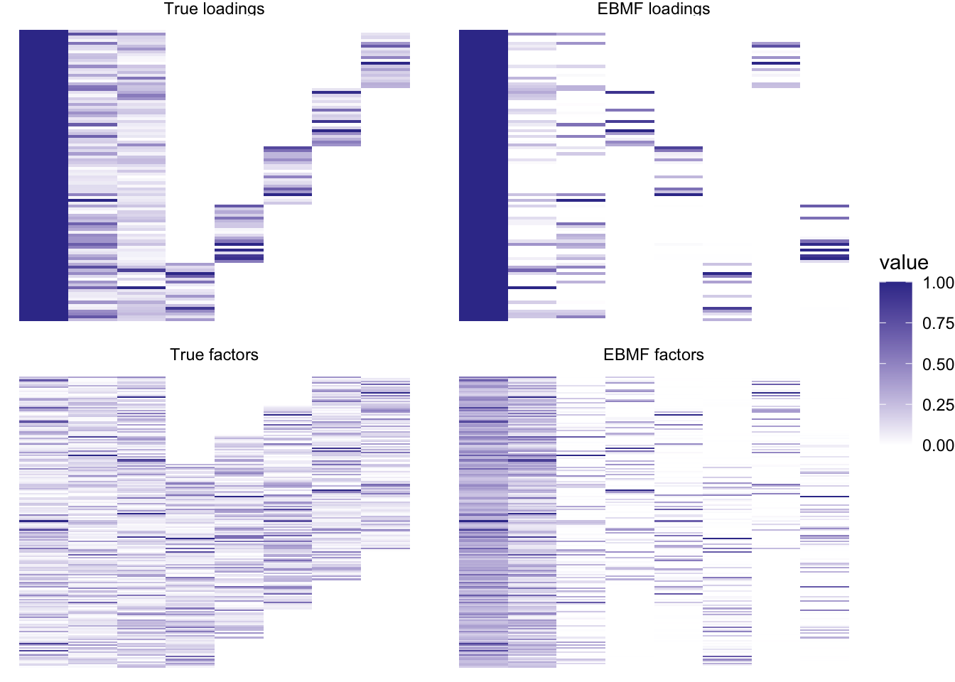
plot_it(simdat, greedy_res)
So it already captures the correct structure, but the loadings and factors are a bit “thinner” or sparser than they should be.
Backfit from greedy
The results using greedy + backfit are as follows. (This method was used in the previous analysis.)
bf_t <- system.time({
  bf_res <- greedy_res %>%
    flash.backfit()
})

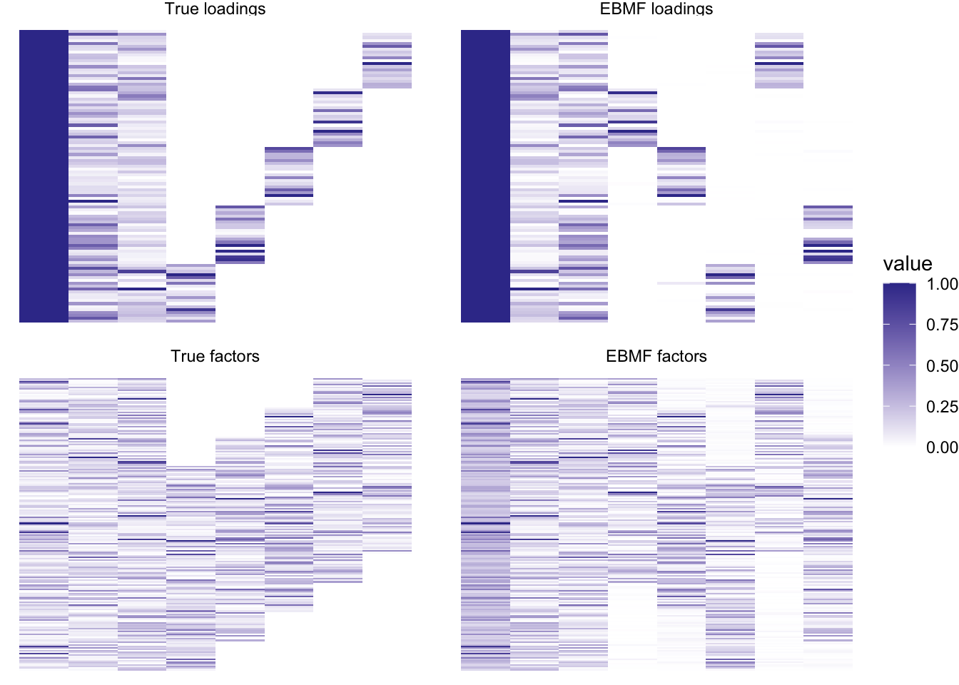
plot_it(simdat, bf_res)
Very nice! And fast – this backfit took only 1.703 seconds.
Backfit from NNLM
Recall from the previous analysis that the nnlm fit is not nearly as clean as the flashier fit. Can EBMF improve upon the nnlm results?
nnmf_res <- NNLM::nnmf(simdat$Y, init = list(W0 = ones), k = 7, verbose = 0)
nnlmbf_t <- system.time({
  nnlmbf_res <- flash.init(simdat$Y) %>%
    flash.set.verbose(0) %>%
    flash.init.factors(
      list(nnmf_res$W[, c(8, 1:7)], t(nnmf_res$H[c(8, 1:7), ])),
      ebnm.fn = ebnm::ebnm_point_exponential
    ) %>%
    flash.fix.factors(kset = 1, mode = 1) %>%
    flash.backfit()
})

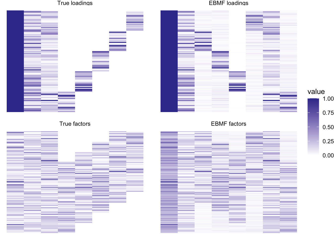
plot_it(simdat, nnlmbf_res)
Still pretty good! Loadings are not exactly sparse, but close enough. This method does take a bit longer: this backfit took 3.795 seconds.
Point-exponential priors with non-zero shift
Can using point-exponential priors with a non-zero mode improve either the fit or the computation time? The greedy + backfit algorithm already works really well on this scenario, so I’ll focus instead on backfitting the nnlm fit.
nzpe_t <- system.time({
  nzpe_res <- flash.init(simdat$Y) %>%
    flash.set.verbose(3) %>%
    flash.init.factors(
      list(nnmf_res$W[, c(8, 1:7)], t(nnmf_res$H[c(8, 1:7), ])),
      ebnm.fn = c(
        as.ebnm.fn(prior_family = "point_exponential", mode = "estimate"),
        ebnm::ebnm_point_exponential
      )
    ) %>%
    flash.fix.factors(kset = 1, mode = 1) %>%
    flash.backfit()
})
#> Convergence tolerance set to 2.98e-04.
#> Backfitting 8 factors (tolerance: 2.98e-04)...
#>     Iteration  Factor   ELBO Diff     Max Chg
#>             1     all          NA    2.39e-02
#>             2     all    8.54e+01   -1.52e-02
#>             3     all    5.24e+01   -1.16e-02
#>             4     all    3.61e+01   -9.74e-03
#>             5     all    2.73e+01   -1.29e-02
#>             6     all    1.95e+01   -1.09e-02
#>             7     all    1.45e+01   -7.95e-03
#>             8     all    1.22e+01   -1.39e-02
#>             9     all    1.07e+01   -1.33e-02
#>            10     all    1.01e+01   -2.19e-02
#>            11     all    8.74e+00    1.28e-02
#>            12     all    7.50e+00   -2.67e-02
#>            13     all    2.94e+00   -2.21e-02
#>            14     all    1.16e+01    7.53e-03
#>            15     all    8.57e+00    8.36e-03
#>            16     all    5.90e+00    9.16e-03
#>            17     all    6.30e+00    9.83e-03
#>            18     all    9.30e+00    1.43e-02
#>            19     all    8.49e+00    2.52e-02
#>            20     all    1.11e+01   -4.30e-03
#>            21     all    1.14e+01   -5.88e-03
#>            22     all    7.92e+00    7.05e-03
#>            23     all    2.08e+00    9.22e-03
#>            24     all    3.29e+00   -3.01e-03
#>            25     all    3.36e+00   -4.18e-03
#>            26     all    3.41e+00   -5.53e-03
#>            27     all    4.29e+00   -5.83e-03
#>            28     all    6.75e+00    7.18e-03
#>            29     all    1.26e+01    1.19e-02
#>            30     all    2.45e+01    2.32e-02
#>            31     all    3.46e+01   -3.56e-02
#>            32     all    8.68e+00    6.29e-03
#>            33     all    7.40e+00   -6.84e-03
#>            34     all    3.57e+00   -8.69e-03
#>            35     all    1.46e+00   -3.88e-03
#>            36     all    1.23e+00    5.20e-03
#>            37     all    1.18e+00    4.87e-03
#>            38     all    1.56e+00    2.98e-03
#>            39     all    2.19e+00    4.53e-03
#>            40     all    3.09e+00    5.16e-03
#>            41     all    4.48e+00   -9.42e-03
#>            42     all    4.51e+00   -1.51e-02
#>            43     all    2.12e+00    7.33e-03
#>            44     all    1.64e+00    9.43e-03
#>            45     all    8.99e-01   -6.82e-03
#>            46     all    1.13e+00   -9.79e-03
#>            47     all    1.22e+00   -1.19e-02
#>            48     all    2.09e+00    9.15e-03
#>            49     all    1.14e+00    8.75e-03
#>            50     all    7.37e-02    9.97e-03
#>            51     all    9.03e-01   -5.95e-03
#>            52     all    5.74e-01   -5.19e-03
#>            53     all    3.46e-01   -4.26e-03
#>            54     all    4.82e-01    3.85e-03
#>            55     all    7.70e-01    4.51e-03
#>            56     all    1.04e+00    6.43e-03
#>            57     all    1.41e+00   -1.14e-02
#>            58     all    1.89e+00   -1.51e-02
#>            59     all    2.12e+00    8.76e-03
#>            60     all    9.06e-01    1.20e-02
#>            61     all    4.31e-01    3.42e-03
#>            62     all    3.05e-01    2.55e-03
#>            63     all    2.34e-01   -2.53e-03
#>            64     all    2.74e-01   -2.01e-03
#>            65     all    3.49e-01   -1.98e-03
#>            66     all    4.70e-01    2.90e-03
#>            67     all    6.97e-01   -2.70e-03
#>            68     all    1.13e+00    3.87e-03
#>            69     all    1.88e+00   -7.25e-03
#>            70     all    2.49e+00   -1.40e-02
#>            71     all    3.07e-01   -2.66e-02
#>            72     all    4.42e+00    9.61e-03
#>            73     all    3.41e+00    1.36e-02
#>            74     all    1.92e+00    1.13e-02
#>            75     all    1.52e+00   -1.62e-02
#>            76     all    2.39e+00   -8.88e-03
#>            77     all    1.34e+00    8.84e-03
#>            78     all    4.83e-01    9.24e-03
#>            79     all    7.15e-01    9.95e-03
#>            80     all    1.27e+00    9.52e-03
#>            81     all    8.99e-01   -1.99e-02
#>            82     all    2.97e+00    9.43e-03
#>            83     all    1.27e+00    1.21e-02
#>            84     all    5.97e-01   -3.76e-03
#>            85     all    4.50e-01   -4.07e-03
#>            86     all    3.99e-01   -2.53e-03
#>            87     all    4.93e-01   -2.45e-03
#>            88     all    6.59e-01   -2.33e-03
#>            89     all    9.39e-01    3.13e-03
#>            90     all    1.46e+00    3.65e-03
#>            91     all    2.58e+00    6.92e-03
#>            92     all    4.96e+00    1.43e-02
#>            93     all    8.59e+00    2.83e-02
#>            94     all    9.26e+00    4.21e-02
#>            95     all    4.52e+00    1.25e-02
#>            96     all    2.46e+00    1.24e-02
#>            97     all    9.23e-01   -4.29e-03
#>            98     all    7.74e-01   -4.93e-03
#>            99     all    5.73e-01   -2.81e-03
#>           100     all    4.94e-01    3.32e-03
#>           101     all    4.08e-01    3.36e-03
#>           102     all    1.81e-01    3.92e-03
#>           103     all    1.75e-01   -2.10e-03
#>           104     all    1.46e-01   -2.48e-03
#>           105     all    1.07e-01    1.68e-03
#>           106     all    1.19e-01    2.10e-03
#>           107     all    1.50e-01    2.12e-03
#>           108     all    1.50e-01    3.11e-03
#>           109     all    8.63e-02    4.42e-03
#>           110     all    2.33e-01   -2.43e-03
#>           111     all    1.66e-01    3.01e-03
#>           112     all    8.04e-02    2.48e-03
#>           113     all    3.70e-02    3.49e-03
#>           114     all    1.31e-01   -2.42e-03
#>           115     all    8.27e-02   -2.47e-03
#>           116     all    3.22e-02   -2.21e-03
#>           117     all    4.06e-02    2.50e-03
#>           118     all    9.20e-02    3.03e-03
#>           119     all    7.38e-02    4.53e-03
#>           120     all    1.74e-01   -2.63e-03
#>           121     all    9.45e-02   -3.55e-03
#>           122     all    3.79e-02    1.09e-03
#>           123     all    3.01e-02    1.08e-03
#>           124     all    2.77e-02    7.98e-04
#>           125     all    3.24e-02    5.58e-04
#>           126     all    4.21e-02   -7.94e-04
#>           127     all    5.92e-02   -8.56e-04
#>           128     all    8.71e-02   -9.46e-04
#>           129     all    1.45e-01    1.55e-03
#>           130     all    2.46e-01    2.47e-03
#>           131     all    2.48e-01   -4.66e-03
#>           132     all    1.21e-01   -2.21e-03
#>           133     all    6.19e-02   -3.04e-03
#>           134     all    1.96e-02    1.00e-03
#>           135     all    1.16e-02    8.52e-04
#>           136     all    5.89e-03    6.49e-04
#>           137     all    3.94e-03    4.67e-04
#>           138     all    4.22e-03   -5.72e-04
#>           139     all    4.62e-03   -7.96e-04
#>           140     all    2.58e-03   -8.42e-04
#>           141     all    1.22e-03   -1.09e-03
#>           142     all    1.74e-02    6.47e-04
#>           143     all    9.28e-03   -1.01e-03
#>           144     all    1.01e-03   -8.75e-04
#>           145     all    6.22e-03   -4.76e-04
#>           146     all    3.29e-03    5.77e-04
#>           147     all    2.04e-03    3.74e-04
#>           148     all    2.69e-03    3.36e-04
#>           149     all    3.73e-03   -5.14e-04
#>           150     all    5.78e-03   -6.33e-04
#>           151     all    6.66e-03   -8.61e-04
#>           152     all    3.38e-03    1.35e-03
#>           153     all    1.80e-02    9.16e-04
#>           154     all    6.90e-03    8.57e-04
#>           155     all    2.85e-03   -2.94e-04
#>           156     all    2.08e-03   -3.46e-04
#>           157     all    1.33e-03   -1.82e-04
#>           158     all    1.41e-03   -1.91e-04
#>           159     all    1.90e-03    2.27e-04
#>           160     all    2.30e-03   -2.15e-04
#>           161     all    3.10e-03   -3.89e-04
#>           162     all    4.94e-03   -4.90e-04
#>           163     all    5.12e-03   -5.56e-04
#>           164     all    5.16e-03    4.51e-04
#>           165     all    3.28e-03    5.83e-04
#>           166     all    1.15e-03    1.88e-04
#>           167     all    9.75e-04    1.45e-04
#>           168     all    8.26e-04   -1.32e-04
#>           169     all    8.25e-04    1.13e-04
#>           170     all    9.47e-04    1.30e-04
#>           171     all    1.15e-03   -1.47e-04
#>           172     all    1.37e-03   -2.21e-04
#>           173     all    1.62e-03   -3.77e-04
#>           174     all    5.89e-04   -7.01e-04
#>           175     all    1.90e-03   -2.74e-04
#>           176     all    1.61e-03   -2.49e-04
#>           177     all    9.49e-04    2.71e-04
#>           178     all    3.77e-04   -3.63e-04
#>           179     all    1.22e-03   -2.31e-04
#>           180     all    6.96e-04   -2.12e-04
#>           181     all    2.39e-04   -8.72e-05
#> Wrapping up...
#> Warning in ebnm_workhorse(x = x, s = s, mode = mode, scale = scale, g_init =
#> g_init, : Since they're not well defined for nonzero modes, local false sign
#> rates won't be returned.

#> Warning in ebnm_workhorse(x = x, s = s, mode = mode, scale = scale, g_init =
#> g_init, : Since they're not well defined for nonzero modes, local false sign
#> rates won't be returned.

#> Warning in ebnm_workhorse(x = x, s = s, mode = mode, scale = scale, g_init =
#> g_init, : Since they're not well defined for nonzero modes, local false sign
#> rates won't be returned.

#> Warning in ebnm_workhorse(x = x, s = s, mode = mode, scale = scale, g_init =
#> g_init, : Since they're not well defined for nonzero modes, local false sign
#> rates won't be returned.

#> Warning in ebnm_workhorse(x = x, s = s, mode = mode, scale = scale, g_init =
#> g_init, : Since they're not well defined for nonzero modes, local false sign
#> rates won't be returned.

#> Warning in ebnm_workhorse(x = x, s = s, mode = mode, scale = scale, g_init =
#> g_init, : Since they're not well defined for nonzero modes, local false sign
#> rates won't be returned.

#> Warning in ebnm_workhorse(x = x, s = s, mode = mode, scale = scale, g_init =
#> g_init, : Since they're not well defined for nonzero modes, local false sign
#> rates won't be returned.
#> Done.

# Shift loadings for visualization purposes.
shifts <- sapply(nzpe_res$L.ghat[2:8], function(g) g$shift[1])
nzpe_res$L.pm[, 2:8] <- nzpe_res$L.pm[, 2:8] - rep(shifts, each = nrow(simdat$Y))

plot_it(simdat, nzpe_res)
I don’t think that these more complicated priors help much in this case, either in terms of the fit or in terms of performance (this backfit took 7.281 seconds). We should try again using a more complex scenario.
sessionInfo()
#> R version 3.5.3 (2019-03-11)
#> Platform: x86_64-apple-darwin15.6.0 (64-bit)
#> Running under: macOS Mojave 10.14.6
#>
#> Matrix products: default
#> BLAS: /Library/Frameworks/R.framework/Versions/3.5/Resources/lib/libRblas.0.dylib
#> LAPACK: /Library/Frameworks/R.framework/Versions/3.5/Resources/lib/libRlapack.dylib
#>
#> locale:
#> [1] en_US.UTF-8/en_US.UTF-8/en_US.UTF-8/C/en_US.UTF-8/en_US.UTF-8
#>
#> attached base packages:
#> [1] stats     graphics  grDevices utils     datasets  methods   base
#>
#> other attached packages:
#>  [1] forcats_0.5.1   stringr_1.4.0   dplyr_1.0.8     purrr_0.3.4
#>  [5] readr_2.0.0     tidyr_1.2.0     tibble_3.1.6    ggplot2_3.3.5
#>  [9] tidyverse_1.3.1 flashier_0.2.27 magrittr_2.0.2  workflowr_1.6.2
#>
#> loaded via a namespace (and not attached):
#>  [1] fs_1.5.0          lubridate_1.7.10  httr_1.4.2        rprojroot_2.0.2
#>  [5] tools_3.5.3       backports_1.1.3   bslib_0.3.1       utf8_1.2.2
#>  [9] R6_2.5.1          irlba_2.3.3       DBI_1.0.0         colorspace_2.0-3
#> [13] withr_2.5.0       tidyselect_1.1.2  compiler_3.5.3    git2r_0.28.0
#> [17] cli_3.2.0         rvest_1.0.0       xml2_1.3.2        labeling_0.4.2
#> [21] horseshoe_0.2.0   sass_0.4.0        scales_1.1.1      SQUAREM_2021.1
#> [25] mixsqp_0.3-43     digest_0.6.29     rmarkdown_2.11    deconvolveR_1.2-1
#> [29] pkgconfig_2.0.3   htmltools_0.5.2   dbplyr_2.1.1      fastmap_1.1.0
#> [33] invgamma_1.1      highr_0.9         rlang_1.0.2       readxl_1.3.1
#> [37] rstudioapi_0.13   jquerylib_0.1.4   generics_0.1.2    farver_2.1.0
#> [41] jsonlite_1.8.0    Matrix_1.3-4      Rcpp_1.0.8        munsell_0.5.0
#> [45] fansi_1.0.2       lifecycle_1.0.1   stringi_1.4.6     whisker_0.3-2
#> [49] yaml_2.3.5        grid_3.5.3        parallel_3.5.3    promises_1.2.0.1
#> [53] crayon_1.5.0      lattice_0.20-38   haven_2.3.1       splines_3.5.3
#> [57] hms_1.1.1         knitr_1.33        pillar_1.7.0      softImpute_1.4-1
#> [61] reprex_2.0.0      glue_1.6.2        evaluate_0.14     trust_0.1-8
#> [65] modelr_0.1.8      vctrs_0.3.8       tzdb_0.1.1        httpuv_1.5.2
#> [69] cellranger_1.1.0  gtable_0.3.0      ebnm_1.0-11       assertthat_0.2.1
#> [73] ashr_2.2-54       xfun_0.29         broom_0.7.6       NNLM_0.4.2
#> [77] later_1.3.0       truncnorm_1.0-8   ellipsis_0.3.2