Backfits

Introduction

Although I’ve done much to speed up backfits, they remain slow relative to greedy fits. The question, then, is whether they’re worth the wait. Here, I’ll argue that while the quantitative improvements are relatively small — one can obtain a similar increase in ELBO in a fraction of the time by greedily adding a few additional factors — the qualitative improvements can be dramatic.

In this analysis, I take the best fit from my analysis of variance structures (the fit that “pre-scales” genes and cells) and compare it against a backfitted version of the same. The code used to produce the fits can be viewed here.

source("./code/utils.R")
droplet <- readRDS("./data/droplet.rds")
processed <- preprocess.droplet(droplet)
res <- readRDS("./output/backfit/flashier_fits.rds")

progress.g <- data.table::fread("./output/backfit/greedy_output.txt")
progress.b <- data.table::fread("./output/backfit/backfit_output.txt")

Improvement in ELBO

As a quantitative measure of how much backfitting improves the fit, I plot the ELBO attained after each of the last five greedy factors have been added and after each of the first 50 backfitting iterations (backfitting continues for a total of 128 iterations, but the ELBO remains level after the first 30 or so iterations).

From this perspective, backfitting offers about as much improvement as the greedy addition of 3-4 factors. However, a single backfitting iteration takes almost 30 seconds, whereas the entire greedy fit can be performed in less than a minute.

g.iter <- nrow(progress.g)
b.iter <- nrow(progress.b)
progress.g$elapsed.time <- (res$t$greedy * 1:g.iter / g.iter) / 60
progress.b$elapsed.time <- (res$t$greedy + res$t$backfit * 1:b.iter / b.iter) / 60

# Only the final iteration for each greedy factor is needed.
progress.g <- subset(progress.g, c((progress.g$Factor[1:(nrow(progress.g) - 1)]
                                    != progress.g$Factor[2:nrow(progress.g)]), TRUE))

progress.df <- rbind(progress.g, progress.b)

ggplot(subset(progress.df, !(Factor %in% as.character(1:15)) & Iter < 50), 
       aes(x = elapsed.time, y = Obj, color = Type)) +
  geom_point() +
  labs(x = "elapsed time (min)", y = "ELBO (unadjusted)",
       title = "Greedy factors 16-20 and first 50 backfitting iterations")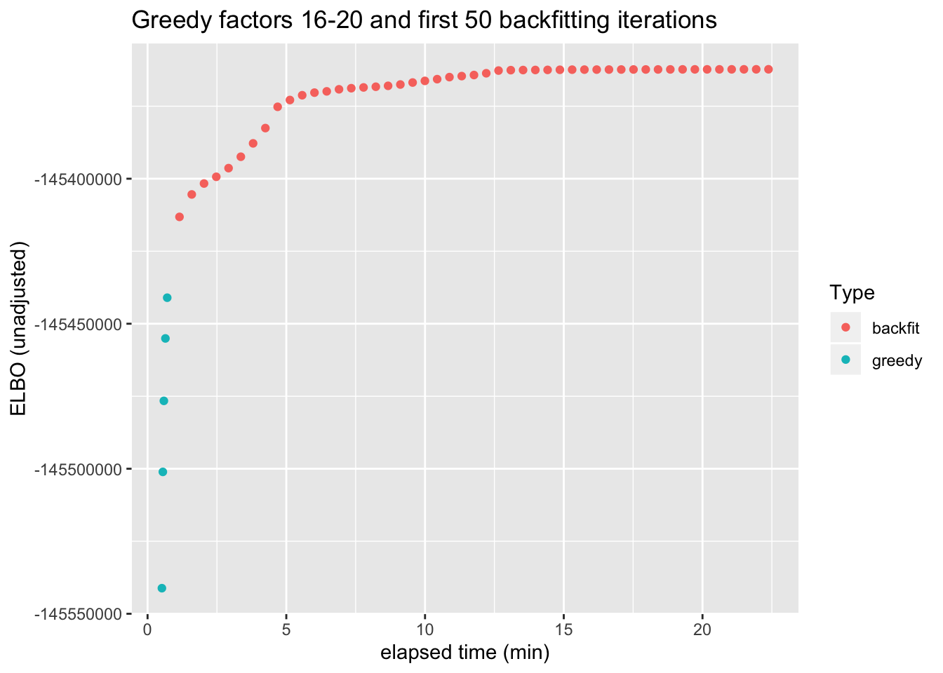

Factor comparison

The ELBO does not tell the whole story. Plotting the factors reveals clear improvements in the backfitted factors. Most obviously, factors 3, 6-8, 11-12, and 17-19 are much sparser and are easily readable as cell-type specific factors. In particular, the unfortunate case of the goblet cells (discussed here) has been cleared up. Factor 2 is also more easily interpretable as indexing a basal-club trajectory without ciliated cells mucking up the situation.

plot.factors(res$fl$greedy, processed$cell.type, title = "Greedy")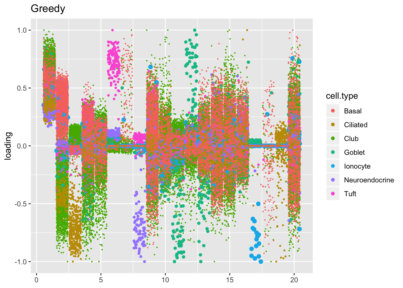

plot.factors(res$fl$backfit, processed$cell.type, title = "Backfit")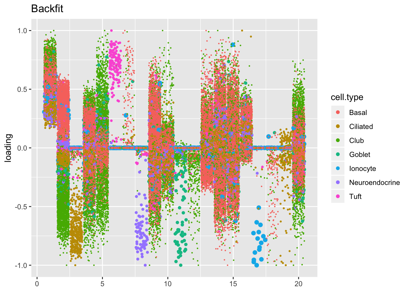

Factors 12 and 13 have increased in importance, while factor 5 (the hillock factor) has become less important. These changes are related: see below. Factors 16, 18, and 20 have also increased in importance (and have possibly borrowed from factor 9), but the significance of these factors is not clear to me.

pve.df <- data.frame(k = 1:res$fl$greedy$n.factors, 
                     greedy = res$fl$greedy$pve, 
                     backfit = res$fl$backfit$pve)
ggplot(pve.df, aes(x = greedy, y = backfit)) +
  geom_text(label = pve.df$k, size = 3) + 
  geom_abline(slope = 1, linetype = "dashed") + 
  scale_x_log10() + scale_y_log10() +
  labs(title = "Proportion of variance explained")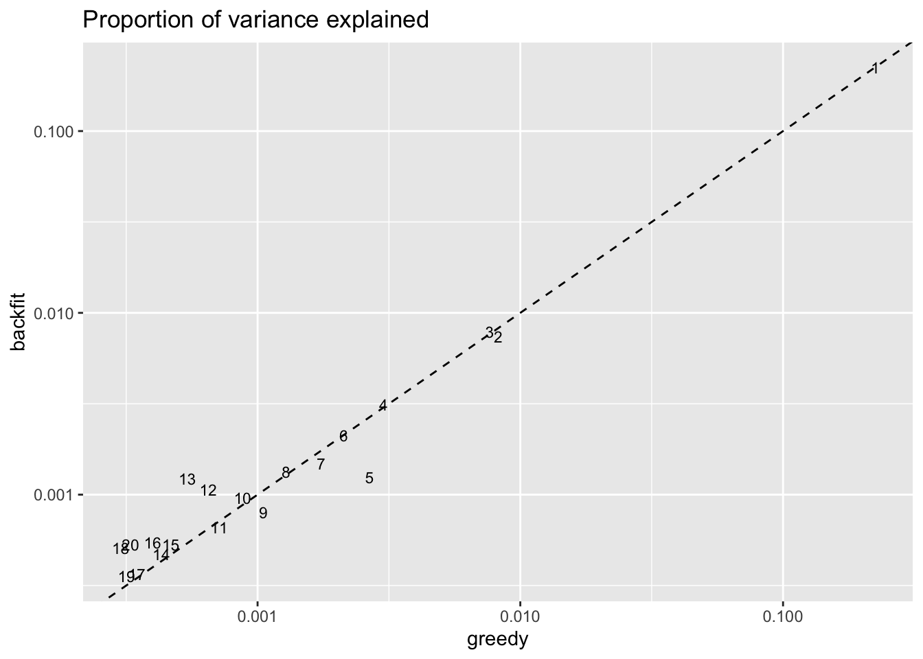

Hillock factor

One of the most interesting changes concerns the “hillock factor.” As far as I can tell, the burden of representing hillock cells is transferred from a single factor (factor 5) to three separate factors (5, 12, and 13). Note, in particular, that Krt13 (a marker gene for hillock cells) has entirely disappeared from the top loadings for factor 5. Instead, the two backfitted factors that are most highly loaded on Krt13 are factors 12 and 13, which are no longer confounded with goblet-specific effects. Intriguingly, factor 12 is almost exclusively loaded on club cells, whereas factor 13 is non-sparse and includes basal and tuft cells.

hillock.genes <- c("Krt13", "Krt4", "Ecm1", "S100a11", "Cldn3", "Lgals3", "Anxa1",
                   "S100a6", "Upk3bl", "Aqp5", "Anxa2", "Crip1", "Gsto1", "Tppp3")

plot.one.factor(res$fl$greedy, 5, hillock.genes, "Factor 5 (greedy)", invert = TRUE)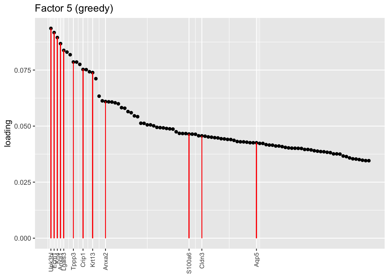

plot.one.factor(res$fl$backfit, 5, hillock.genes, "Factor 5 (backfit)", invert = TRUE)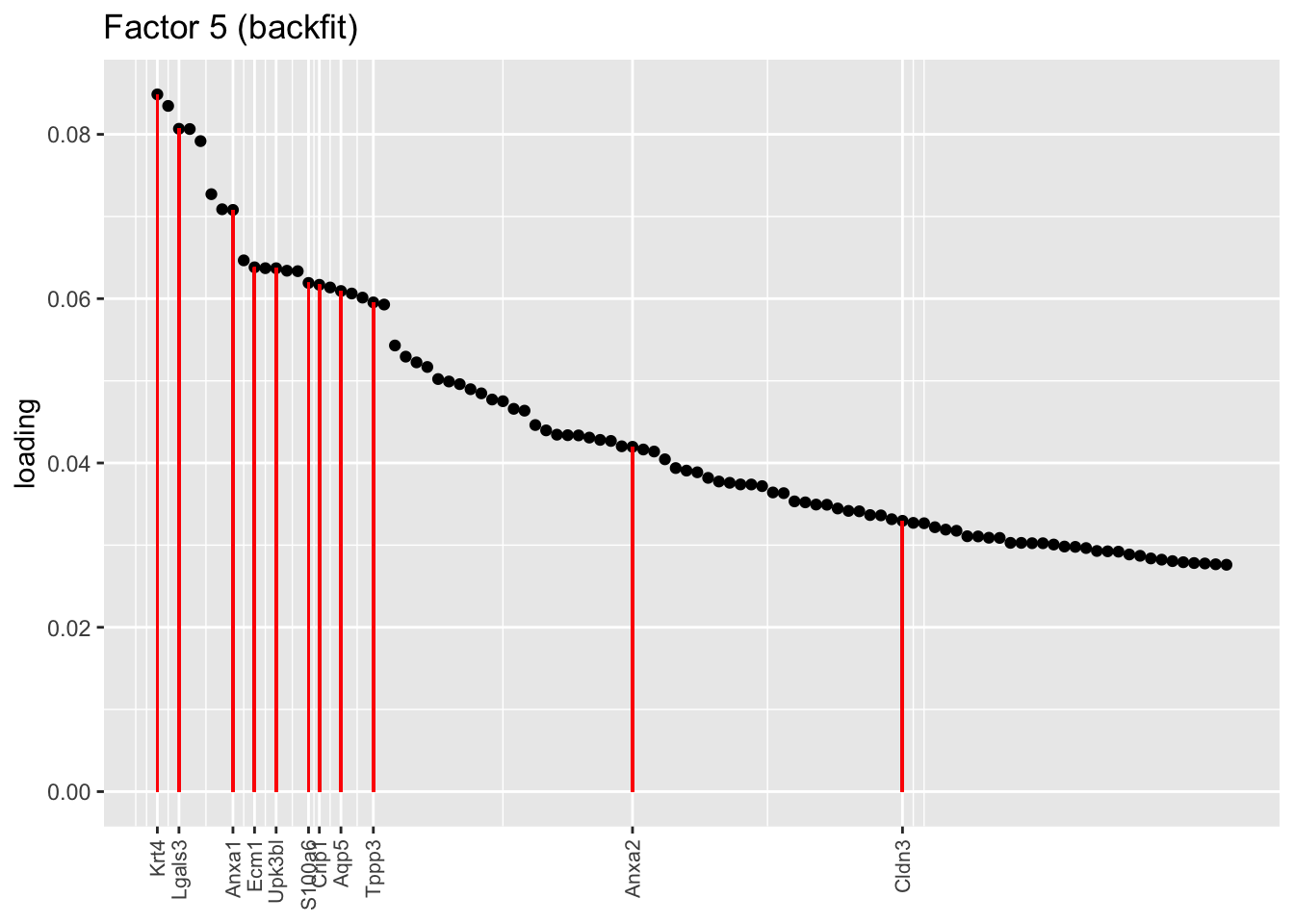

plot.one.factor(res$fl$backfit, 12, hillock.genes, "Factor 12 (backfit)", invert = TRUE)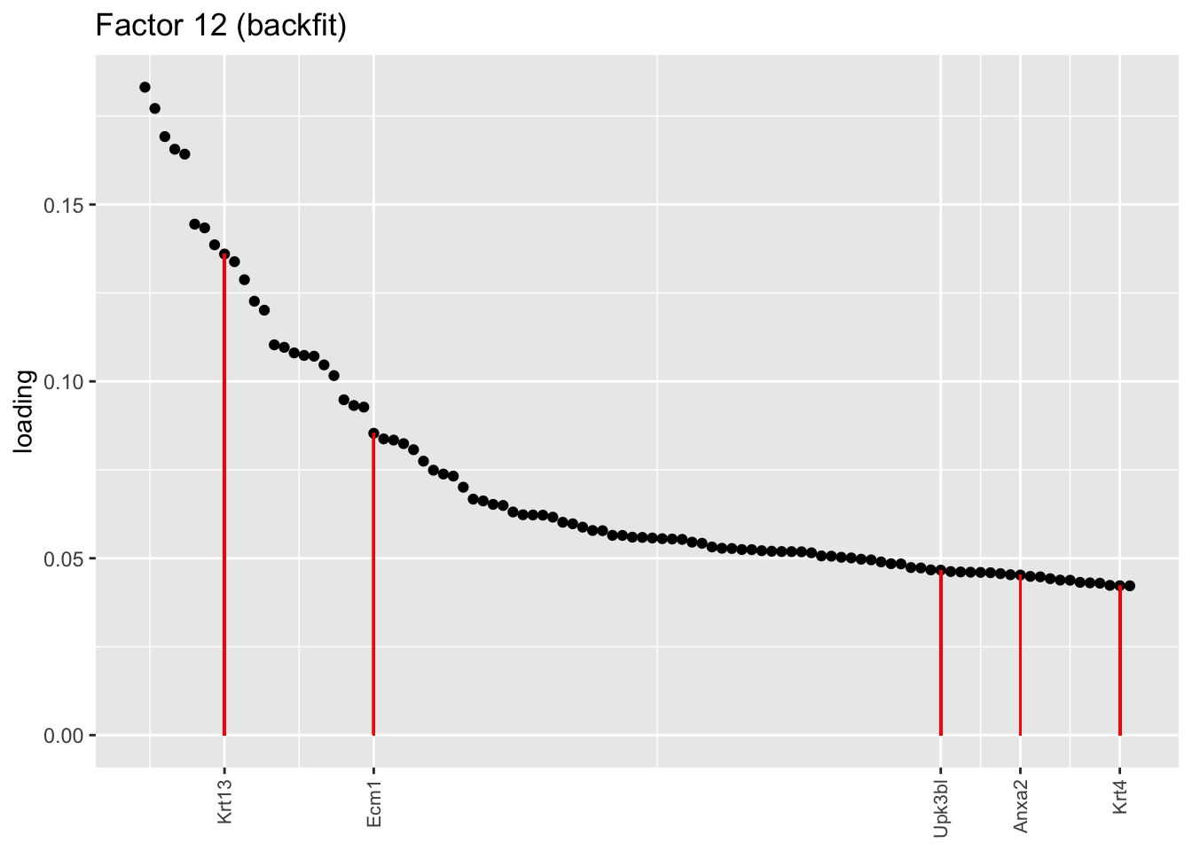

plot.one.factor(res$fl$backfit, 13, hillock.genes, "Factor 13 (backfit)", invert = FALSE)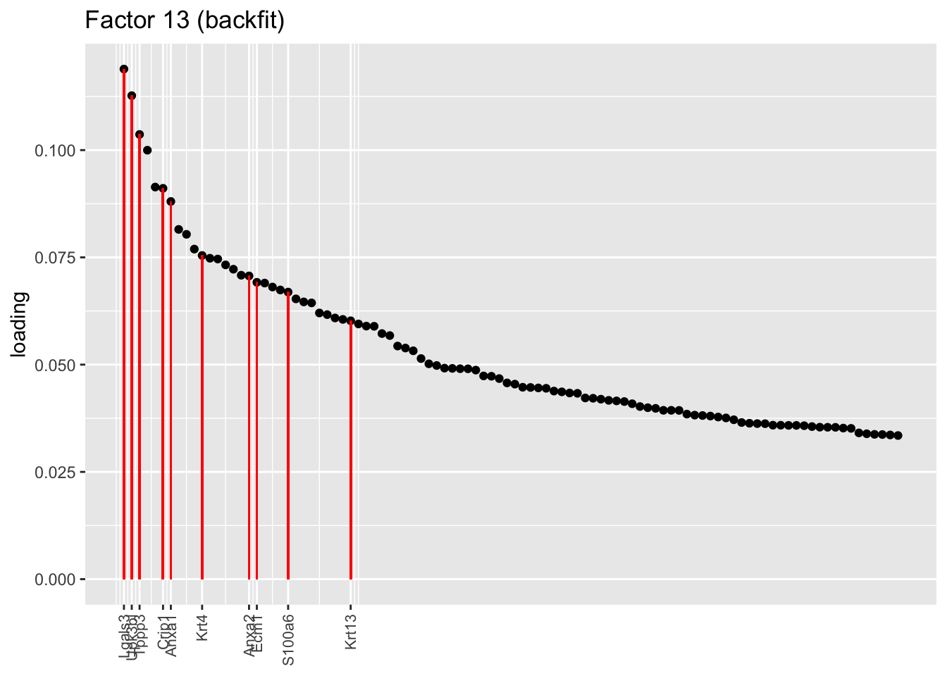

Session information

sessionInfo()

R version 3.5.3 (2019-03-11)
Platform: x86_64-apple-darwin15.6.0 (64-bit)
Running under: macOS Mojave 10.14.6

Matrix products: default
BLAS: /Library/Frameworks/R.framework/Versions/3.5/Resources/lib/libRblas.0.dylib
LAPACK: /Library/Frameworks/R.framework/Versions/3.5/Resources/lib/libRlapack.dylib

locale:
[1] en_US.UTF-8/en_US.UTF-8/en_US.UTF-8/C/en_US.UTF-8/en_US.UTF-8

attached base packages:
[1] stats     graphics  grDevices utils     datasets  methods   base     

other attached packages:
[1] flashier_0.1.11 ggplot2_3.2.0   Matrix_1.2-15  

loaded via a namespace (and not attached):
 [1] Rcpp_1.0.1        plyr_1.8.4        compiler_3.5.3   
 [4] pillar_1.3.1      git2r_0.25.2      workflowr_1.2.0  
 [7] iterators_1.0.10  tools_3.5.3       digest_0.6.18    
[10] evaluate_0.13     tibble_2.1.1      gtable_0.3.0     
[13] lattice_0.20-38   pkgconfig_2.0.2   rlang_0.3.1      
[16] foreach_1.4.4     parallel_3.5.3    yaml_2.2.0       
[19] ebnm_0.1-24       xfun_0.6          withr_2.1.2      
[22] stringr_1.4.0     dplyr_0.8.0.1     knitr_1.22       
[25] fs_1.2.7          rprojroot_1.3-2   grid_3.5.3       
[28] tidyselect_0.2.5  data.table_1.12.2 glue_1.3.1       
[31] R6_2.4.0          rmarkdown_1.12    mixsqp_0.1-119   
[34] reshape2_1.4.3    ashr_2.2-38       purrr_0.3.2      
[37] magrittr_1.5      whisker_0.3-2     MASS_7.3-51.1    
[40] codetools_0.2-16  backports_1.1.3   scales_1.0.0     
[43] htmltools_0.3.6   assertthat_0.2.1  colorspace_1.4-1 
[46] labeling_0.3      stringi_1.4.3     pscl_1.5.2       
[49] doParallel_1.0.14 lazyeval_0.2.2    munsell_0.5.0    
[52] truncnorm_1.0-8   SQUAREM_2017.10-1 crayon_1.3.4