Pseudocounts

Introduction

In the previous analysis, I argued that it’s best to use a more sophisticated approach to calculating size factors (such as scran). It remains to choose a pseudocount. That is, letting \(X\) be the matrix of scaled counts, I consider the family of transformations \[ Y_{ij} = \log \left( X_{ij} + \alpha \right), \] which is, up to a constant, equivalent to the family of sparsity-preserving transformations \[ Y_{ij} = \log \left( \frac{X_{ij}}{\alpha} + 1 \right). \]

Typical choices of \(\alpha\) include 0.5 and 1. Aaron Lun has argued that a somewhat larger pseudocount should be used. Specifically, he proposes setting \[ \alpha = \min \left\{1, 1/s_\min - 1 / s_\max \right\}, \] where \(s_\min\) and \(s_\max\) are the smallest and largest size factors. Using the scran size factors from the previous analysis, this would yield \(\alpha = 3.14\) .

Here I consider a broader range of \(\alpha\), including pseudocounts that are much smaller (\(\alpha = 1/100\)) and larger (\(\alpha = 100\)) than are probably reasonable.

source("./code/utils.R")
droplet <- readRDS("./data/droplet.rds")
droplet <- preprocess.droplet(droplet)
res <- readRDS("./output/pseudocount/pseudocount_fits.rds")

Previous results

In a previous exploration of pseudocounts, I made the following observations:

• The ELBO is monotonically decreasing as a function of the pseudocount.
• Comparing fits by randomly deleting data, imputing the missing values, and then calculating the Spearman rank correlation between the imputed and true values suggests that an \(\alpha\) between 0.35 and 1 is best.
• Smaller pseudocounts will more strongly shrink small counts, while larger pseudocounts more strongly shrink large counts. The transition between “small” and “large” counts is around 10.
• Smaller pseudocounts favor larger loadings for sparser genes, while larger pseudocounts favor more highly expressed genes.
• One can make a theoretical argument for \(\alpha = 0.5\), but the argument is admittedly pretty flimsy on its own.

Intuition

It’s useful to think about how the EBMF fit will change as \(\alpha\) becomes very small or very large.

As \(\alpha \to 0\), the differences between zero and nonzero counts are accentuated, while the respective differences among nonzero counts diminish in importance. In the limit, the transformed matrix becomes binary. Thus, a smaller \(\alpha\) prioritizes fitting zero counts over carefully distinguishing among nonzero counts.

At the other end of the scale, as \(\alpha\) increases, a larger range of counts is pushed towards zero, which amplifies the difference between large counts and small to moderate counts. As a result, a larger \(\alpha\) prioritizes fitting large counts over getting zero counts exactly right.

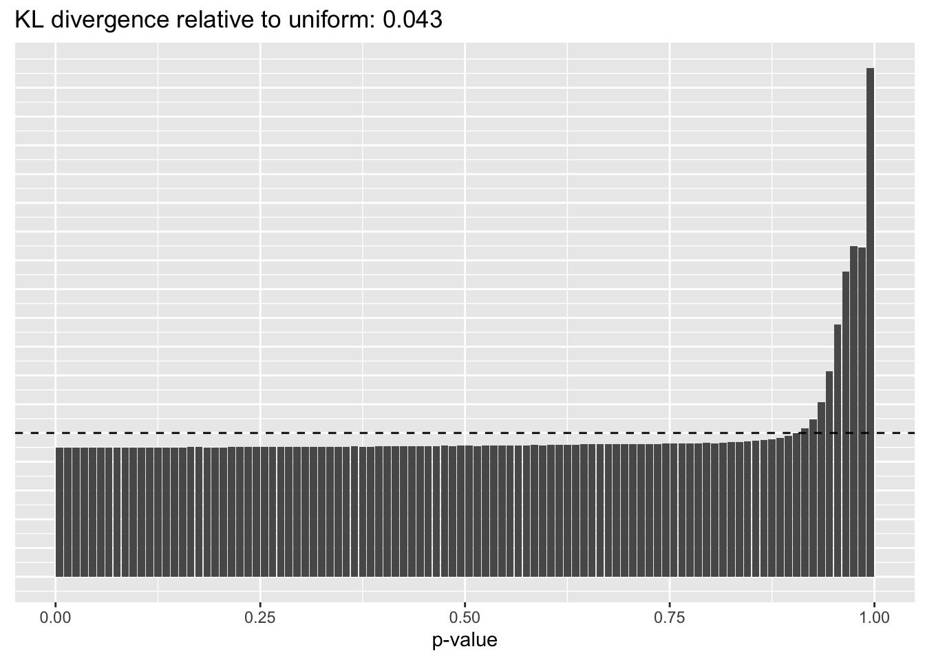
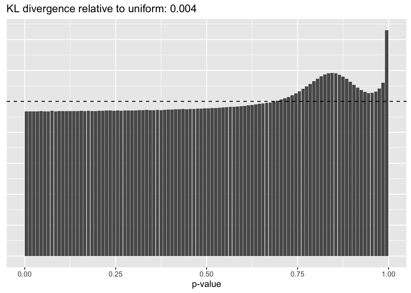
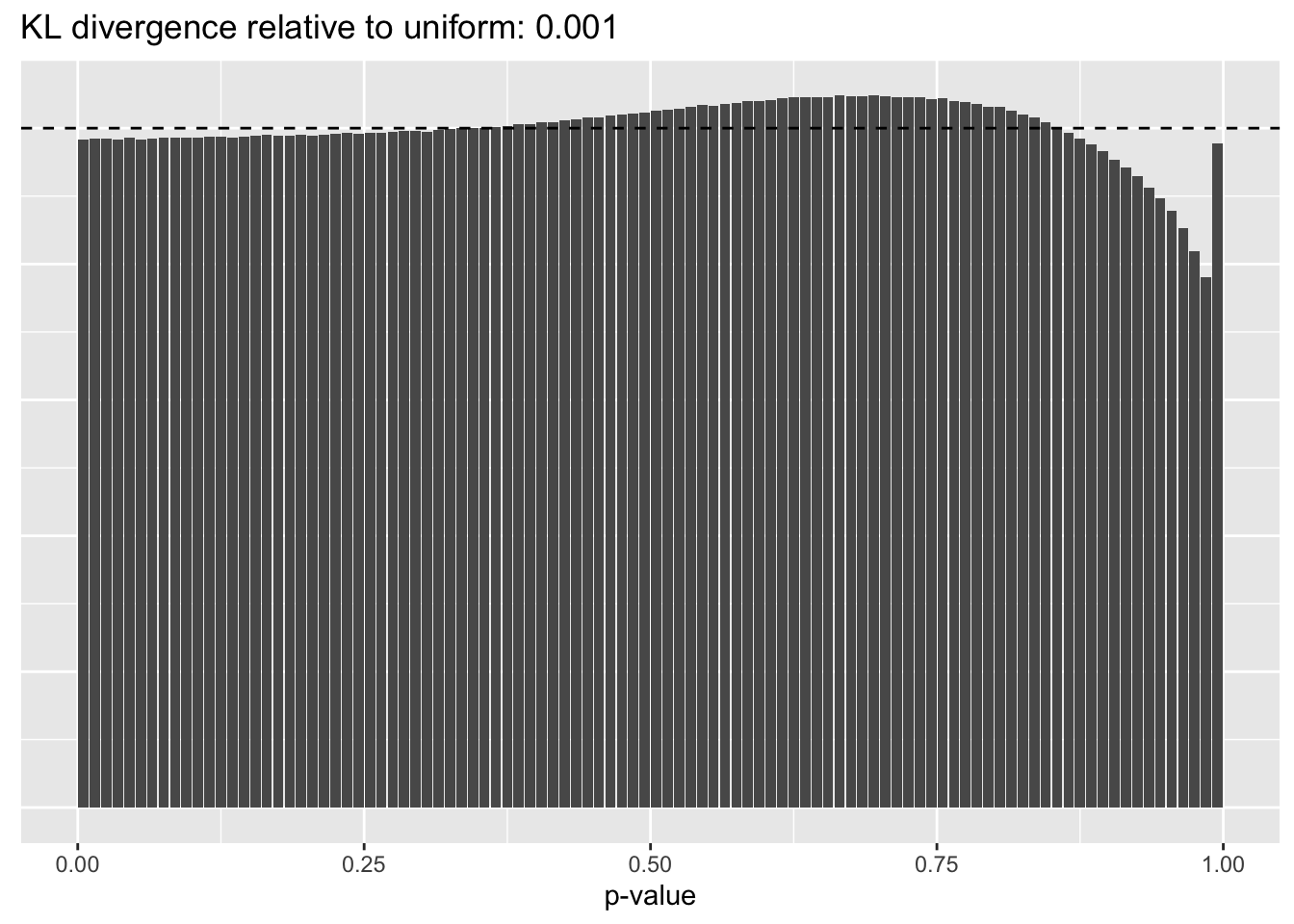
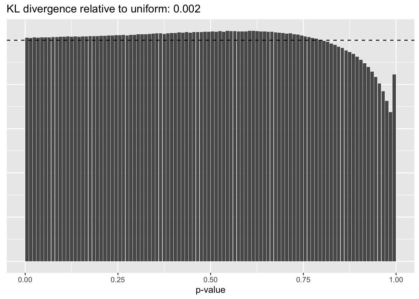
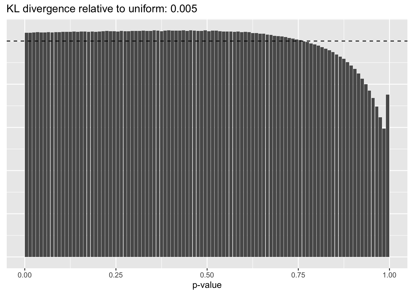
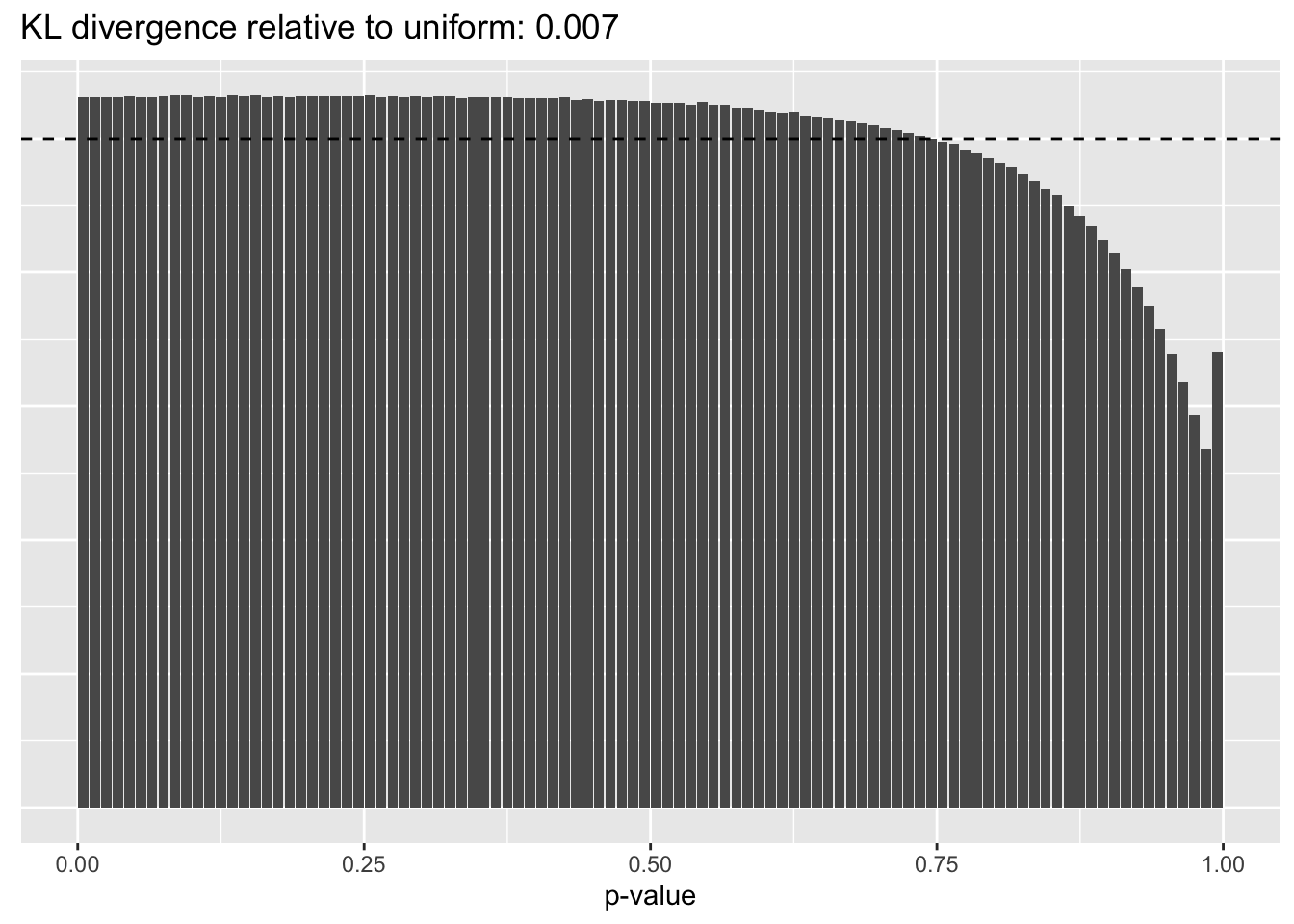
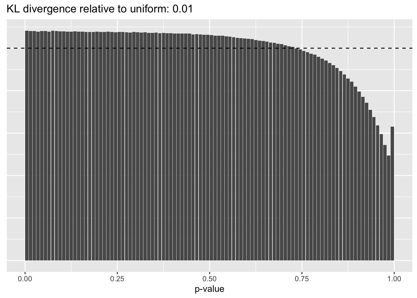
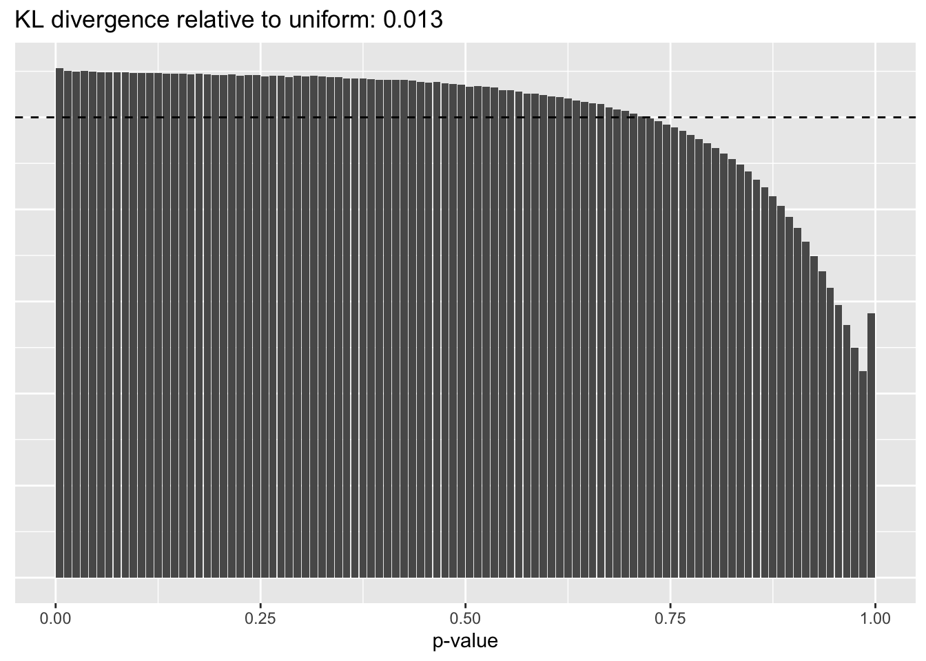
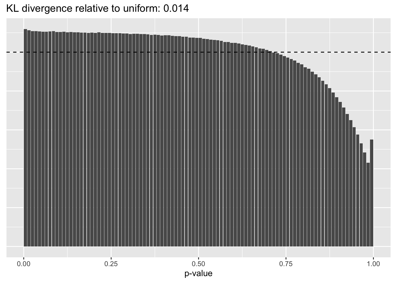
Results: p-values

This intuition is confirmed by the \(p\)-value plots. \(p\)-values near one correspond to fitted values that are much smaller than the true counts, so an overabundance of \(p\)-values near one means that the fitted model is not doing a very good job of fitting large counts. Vice versa, an overabundance of \(p\)-values near zero means that the fitted model is failing to fit zero counts very well. Although I’ve provided the KL divergence between the observed and expected \(p\)-value distributions, it’s not a great metric. In particular, it doesn’t penalize severe under-predictions (\(p \approx 1\)) as much as I’d like.

for (pc in names(res)) {
  cat("\n### Pseudocount = ", pc, "\n")
  plot(plot.p.vals(res[[pc]][["p.vals"]]))
  cat("\n")
}

Results: ELBO

The ELBO is a terrible metric here. Indeed, as I’ve already observed, the ELBO is monotonically decreasing as a function of the pseudocount.

To see why this is the case, imagine fitting a simple rank-one model with a constant variance structure. The data log likelihood (that is, the part of the ELBO that ignores priors) is \[ -\frac{np}{2} \log(2 \pi \sigma^2) - \frac{1}{2 \sigma^2} \sum_{i, j} \mathbb{E} (Y_{ij} - \hat{Y}_{ij})^2. \] Recall that \(\sigma^2\) is estimated (via ML) as the mean expected squared residual, so that the data log likelihood can be written \[ -\frac{np}{2} \log(2 \pi \sigma^2) - \frac{np}{2} = -np \log \sigma + C.\] Meanwhile, the change-of-variables adjustment to the ELBO is \[ np \log (1 / \lambda) - \sum_{i, j} Y_{ij}. \]

Now take \(\lambda \to 0\). Zero entries in \(X\) are always zero in the transformed matrix \(Y\), and nonzero entries are approximately \(\log X_{ij} - \log \lambda \approx -\log \lambda\), so \[ \sum_{i, j} Y_{ij} \approx snp \log (1 / \lambda), \] where \(s\) is the sparsity of \(X\) (that is, the proportion of entries that are nonzero). Next, since the rank-one fit will yield a \(\sigma^2\) that is approximately equal to \(\text{Var}(Y)\), which (in the limit) is \((\log (1 / \lambda))^2 s(1 - s)\), the data log likelihood is approximately \[ -np \log (\sqrt{s} \log (1 / \lambda)) + C = -np \log \log (1 / \lambda) + C. \]

Thus, for \(\lambda\) near zero, the adjusted log likelihood is approximately \[ (1 + s)np \log (1 / \lambda) - np \log \log (1 / \lambda) + C, \] which blows up as \(\lambda \to 0\).

elbo.df <- data.frame(pseudocount = as.numeric(names(res)),
                      elbo = sapply(res, function(x) x$fl$elbo + x$elbo.adj))
ggplot(elbo.df, aes(x = pseudocount, y = elbo)) +
  geom_point() +
  scale_x_continuous(trans = "log2") +
  labs(y = "ELBO")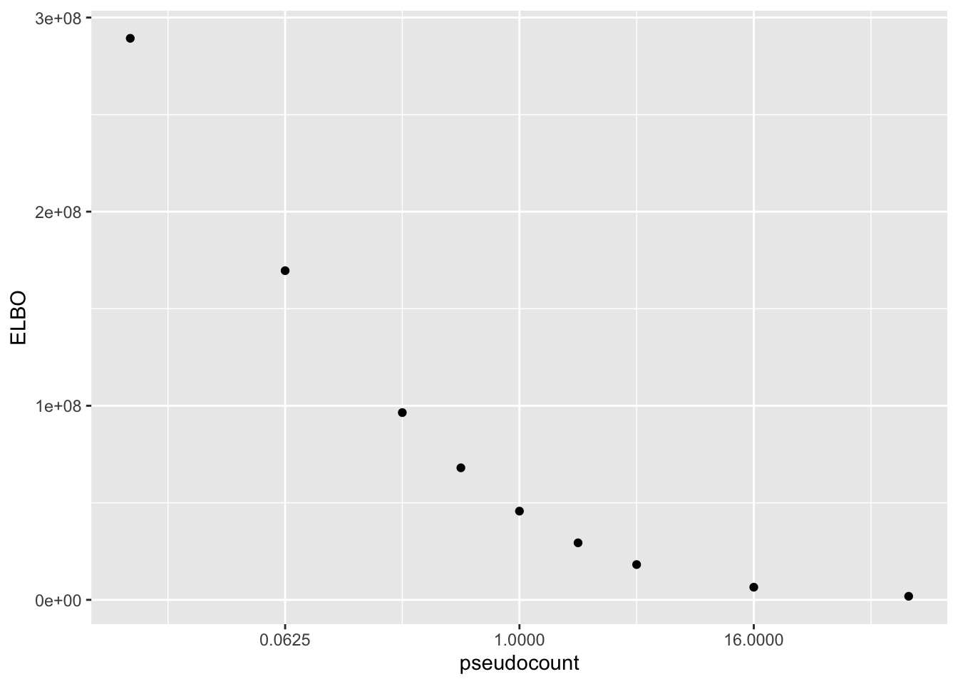

Results: Log likelihood of implied distribution

The log likehood of the implied discrete distribution is a much better metric than the ELBO or the KL-divergence of \(p\)-value distributions. Using this metric, \(\alpha = 0.5\) does best.

llik.df <- data.frame(pseudocount = as.numeric(names(res)),
                      llik = sapply(res, function(x) x$p.vals$llik))
ggplot(llik.df, aes(x = pseudocount, y = llik)) +
  geom_point() +
  scale_x_continuous(trans = "log2") +
  labs(y = "log likelihood (implied model)")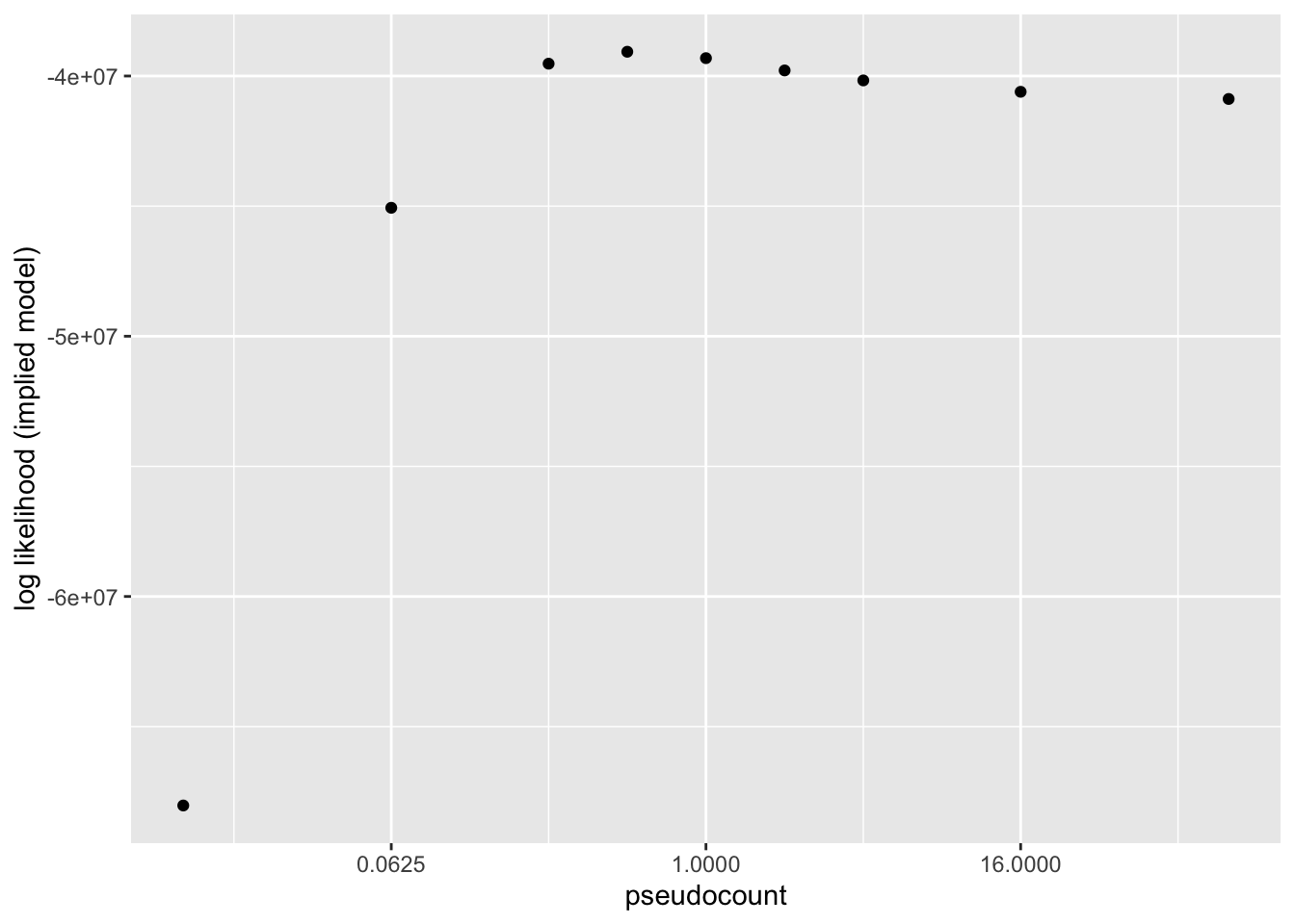

Session information

sessionInfo()

R version 3.5.3 (2019-03-11)
Platform: x86_64-apple-darwin15.6.0 (64-bit)
Running under: macOS Mojave 10.14.6

Matrix products: default
BLAS: /Library/Frameworks/R.framework/Versions/3.5/Resources/lib/libRblas.0.dylib
LAPACK: /Library/Frameworks/R.framework/Versions/3.5/Resources/lib/libRlapack.dylib

locale:
[1] en_US.UTF-8/en_US.UTF-8/en_US.UTF-8/C/en_US.UTF-8/en_US.UTF-8

attached base packages:
[1] stats     graphics  grDevices utils     datasets  methods   base     

other attached packages:
[1] flashier_0.1.15 ggplot2_3.2.0   Matrix_1.2-15  

loaded via a namespace (and not attached):
 [1] Rcpp_1.0.1        compiler_3.5.3    pillar_1.3.1     
 [4] git2r_0.25.2      workflowr_1.2.0   iterators_1.0.10 
 [7] tools_3.5.3       digest_0.6.18     evaluate_0.13    
[10] tibble_2.1.1      gtable_0.3.0      lattice_0.20-38  
[13] pkgconfig_2.0.2   rlang_0.3.1       foreach_1.4.4    
[16] parallel_3.5.3    yaml_2.2.0        ebnm_0.1-24      
[19] xfun_0.6          withr_2.1.2       stringr_1.4.0    
[22] dplyr_0.8.0.1     knitr_1.22        fs_1.2.7         
[25] rprojroot_1.3-2   grid_3.5.3        tidyselect_0.2.5 
[28] glue_1.3.1        R6_2.4.0          rmarkdown_1.12   
[31] mixsqp_0.1-119    ashr_2.2-38       purrr_0.3.2      
[34] magrittr_1.5      whisker_0.3-2     MASS_7.3-51.1    
[37] codetools_0.2-16  backports_1.1.3   scales_1.0.0     
[40] htmltools_0.3.6   assertthat_0.2.1  colorspace_1.4-1 
[43] labeling_0.3      stringi_1.4.3     pscl_1.5.2       
[46] doParallel_1.0.14 lazyeval_0.2.2    munsell_0.5.0    
[49] truncnorm_1.0-8   SQUAREM_2017.10-1 crayon_1.3.4