Prior families
Jason Willwerscheid
8/18/2019
Last updated: 2019-08-21
Checks: 6 0
Knit directory: scFLASH/
This reproducible R Markdown analysis was created with workflowr (version 1.2.0). The Report tab describes the reproducibility checks that were applied when the results were created. The Past versions tab lists the development history.
Great! Since the R Markdown file has been committed to the Git repository, you know the exact version of the code that produced these results.
Great job! The global environment was empty. Objects defined in the global environment can affect the analysis in your R Markdown file in unknown ways. For reproduciblity it’s best to always run the code in an empty environment.
The command set.seed(20181103) was run prior to running the code in the R Markdown file. Setting a seed ensures that any results that rely on randomness, e.g. subsampling or permutations, are reproducible.
Great job! Recording the operating system, R version, and package versions is critical for reproducibility.
Nice! There were no cached chunks for this analysis, so you can be confident that you successfully produced the results during this run.
Great! You are using Git for version control. Tracking code development and connecting the code version to the results is critical for reproducibility. The version displayed above was the version of the Git repository at the time these results were generated.
Note that you need to be careful to ensure that all relevant files for the analysis have been committed to Git prior to generating the results (you can use wflow_publish or wflow_git_commit). workflowr only checks the R Markdown file, but you know if there are other scripts or data files that it depends on. Below is the status of the Git repository when the results were generated:
Ignored files:
    Ignored:    .DS_Store
    Ignored:    .Rhistory
    Ignored:    .Rproj.user/
    Ignored:    data/droplet.rds
    Ignored:    output/backfit/
    Ignored:    output/var_type/

Untracked files:
    Untracked:  analysis/NBapprox.Rmd
    Untracked:  analysis/pseudocount2.Rmd
    Untracked:  analysis/trachea4.Rmd
    Untracked:  code/missing_data.R
    Untracked:  code/prior_type/
    Untracked:  code/pseudocounts.R
    Untracked:  code/trachea4.R
    Untracked:  data/Ensembl2Reactome.txt
    Untracked:  data/hard_bimodal1.txt
    Untracked:  data/hard_bimodal2.txt
    Untracked:  data/hard_bimodal3.txt
    Untracked:  data/mus_pathways.rds
    Untracked:  docs/figure/pseudocount2.Rmd/
    Untracked:  output/prior_type/
    Untracked:  output/pseudocount/

Unstaged changes:
    Modified:   analysis/pseudocount.Rmd
    Modified:   code/sc_comparisons.R
    Modified:   code/utils.R
Note that any generated files, e.g. HTML, png, CSS, etc., are not included in this status report because it is ok for generated content to have uncommitted changes.
These are the previous versions of the R Markdown and HTML files. If you’ve configured a remote Git repository (see ?wflow_git_remote), click on the hyperlinks in the table below to view them.
| File | Version | Author | Date | Message |
|---|---|---|---|---|
| Rmd | ea3518e | Jason Willwerscheid | 2019-08-21 | wflow_publish(“analysis/prior_type.Rmd”) |
Introduction
Here I consider the choice of prior families for the priors \(g_\ell^{(k)}\) and \(g_f^{(k)}\) in the EBMF model \[ Y = LF' + E,\ L_{ik} \sim g_\ell^{(k)},\ F_{jk} \sim g_f^{(k)}. \]
The default prior family in flashier is the two-parameter family of point-normal priors \[ \pi_0 \delta_0 + (1 - \pi_0) N(0, \sigma^2). \] Another choice uses ashr to fit a scale mixture of normals (with mean zero). Since the family of point-normal priors is contained in the family of scale mixtures of normals, using the latter is guaranteed to improve the fit. Computation is a bit slower, but improvements to mixsqp and ebnm have narrowed the gap: my recent benchmarking results suggest that fitting point-normal priors is a little less than twice as fast as fitting scale-mixture-of-normal priors (and for very large datasets, the gap is even smaller).
In addition to point-normal and scale-mixture-of-normal priors, I consider two semi-nonnegative factorizations obtained via the family of priors with nonnegative support and a unique mode at zero. One factorization puts the nonnegative prior on cell loadings with a point-normal prior on gene loadings; the other puts the nonnegative prior on gene loadings (with a point-normal prior on cell loadings).
source("./code/utils.R")
droplet <- readRDS("./data/droplet.rds")
processed <- preprocess.droplet(droplet)
res <- readRDS("./output/prior_type/flashier_fits.rds")
Semi-nonnegative factorizations and interpretability
In my view, the primary advantage of a semi-nonnegative fit is that it enhances interpretability. With a nonnegative prior on cell loadings, interpretation of factors is straightforward: the gene loadings give one set of genes that is overexpressed relative to the mean and another set that is simultaneously underexpressed, and the cell loadings give the cells in which this pattern of over- and underexpression occurs. Similarly, a nonnegative prior on gene loadings gives sets of genes that co-express and cells where this set of genes is either over- or underexpressed.
Without any nonnegative prior, interpretation is less natural. Take the above interpretation of gene loadings as a pattern of over- and underexpression: if cell loadings are no longer constrained to be nonnegative, then one is forced to read the pattern in two ways, so that gene set A is overexpressed and gene set B is underexpressed in some cells, while A is underexpressed and B is overexpressed in other cells. Not only does this impede interpretation, but it doesn’t seem plausible to me that patterns of over- and underexpression would be simple mirror images of one another.
Results: fitting time
Total fitting time is heavily dependent on the number of backfitting iterations required. In particular, the semi-nonnegative fits can be quite slow to converge.
format.t <- function(t) {
  return(sapply(t, function(x) {
    hrs <- floor(x / 3600)
    min <- floor((x - 3600 * hrs) / 60)
    sec <- floor(x - 3600 * hrs - 60 * min)
    if (hrs > 0) {
      return(sprintf("%02.fh%02.fm%02.fs", hrs, min, sec))
    } else if (min > 0) {
      return(sprintf("%02.fm%02.fs", min, sec))
    } else {
      return(sprintf("%02.fs", sec))
    }
  }))
}

t.greedy <- sapply(lapply(res, `[[`, "t"), `[[`, "greedy")
t.backfit <- sapply(lapply(res, `[[`, "t"), `[[`, "backfit")
niter.backfit <- sapply(lapply(res, `[[`, "output"), function(x) x$Iter[nrow(x)])
t.periter.b <- t.backfit / niter.backfit
time.df <- data.frame(format.t(t.greedy), format.t(t.backfit),
                      niter.backfit, format.t(t.periter.b))
rownames(time.df) <- c("Point-normal", "Scale mixture of normals",
                       "Semi-nonnegative (NN cells)", "Semi-nonnegative (NN genes)")
knitr::kable(time.df[c(1, 2, 4, 3), ],
             col.names = c("Greedy time", "Backfit time",
                           "Backfit iter", "Backfit time per iter"),
             digits = 2,
align = "r")| Greedy time | Backfit time | Backfit iter | Backfit time per iter | |
|---|---|---|---|---|
| Point-normal | 01m24s | 58m05s | 88 | 39s |
| Scale mixture of normals | 03m53s | 52m01s | 64 | 48s |
| Semi-nonnegative (NN genes) | 06m41s | 02h48m19s | 146 | 01m09s |
| Semi-nonnegative (NN cells) | 03m16s | 04h58m09s | 345 | 51s |
Results: ELBO
I show the ELBO after each of the last twenty greedy factors have been added and after each of the first 75 backfitting iterations (all ELBOs remain pretty much flat afterwards). snn.cell denotes the semi-nonnegative fit that puts nonnegative priors on cell loadings, whereas snn.gene puts nonnegative priors on gene loadings.
I make the following observations:
Backfitting always results in a substantial improvement, but it is crucial for the semi-nonnegative fits. In effect, backfitting improves the ELBO of the semi-nonnegative fits by nearly as much as the last twenty greedy factors combined, whereas it only improves the point-normal and scale-mixture-of-normal fits by the equivalent of about ten greedy factors.
The difference among the final ELBOs is, in a relative sense, surprisingly small. For example, the gap between the final ELBO for the point-normal fit and for the semi-nonnegative fit with a nonnegative prior on gene loadings is the equivalent of about two or three greedy factors. This suggests that, in some sense, the semi-nonnegative model is closer to biological reality (if loadings were truly point-normal, then the semi-nonnegative fits would require twice as many factors as the point-normal fits).
Putting a nonnegative prior on gene loadings works slightly better here than putting it on cell loadings, but it’d be hasty to generalize. Indeed, note that the relative rank of the two fits changes over the course of the greedy fit. Further investigation is called for.
res$pn$output$Fit <- "pn"
res$ash$output$Fit <- "ash"
res$snn.cell$output$Fit <- "snn.cell"
res$snn.gene$output$Fit <- "snn.gene"

res$pn$output$row <- 1:nrow(res$pn$output)
res$ash$output$row <- 1:nrow(res$ash$output)
res$snn.cell$output$row <- 1:nrow(res$snn.cell$output)
res$snn.gene$output$row <- 1:nrow(res$snn.gene$output)

elbo.df <- rbind(res$pn$output, res$ash$output, res$snn.cell$output, res$snn.gene$output)
ggplot(subset(elbo.df, !(Factor %in% as.character(1:10)) & Iter < 75),
       aes(x = row, y = Obj, color = Type, shape = Fit)) +
  geom_point() +
  labs(x = NULL, y = "elbo",
       title = "Greedy factors 11-30 and first 75 backfitting iterations") +
  theme(axis.text.x = element_blank(), axis.ticks.x = element_blank())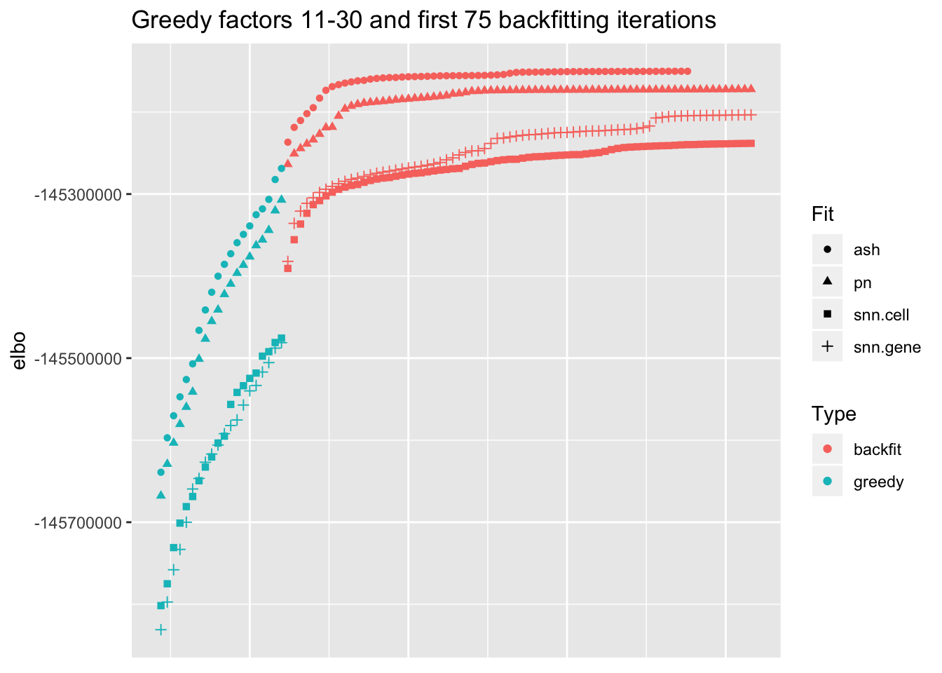
Results: point-normal priors vs. scale mixtures of normals
I plot the point-normal factors in order of proportion of variance explained, and I line up the scale-mixture-of-normal factors so that similar factors are shown one on top of the other. Results are nearly identical.
pn.v.ash  <- compare.factors(res$pn$fl, res$ash$fl)
pn.order  <- match(order(res$pn$fl$pve, decreasing = TRUE), pn.v.ash$fl1.k)
ash.order <- match(order(res$pn$fl$pve, decreasing = TRUE), pn.v.ash$fl2.k)
plot.factors(res$pn$fl, processed$cell.type, pn.order[1:15],
             title = "Point-normal priors (factors 1-15)")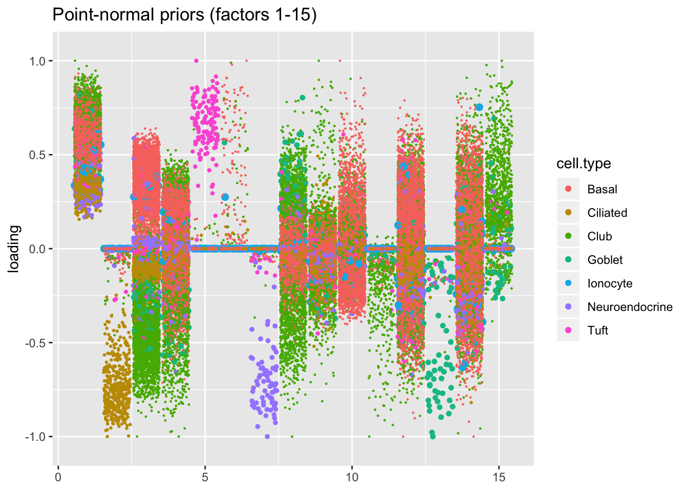
plot.factors(res$ash$fl, processed$cell.type, ash.order[1:15],
             title = "Scale mixtures of normals (factors 1-15)")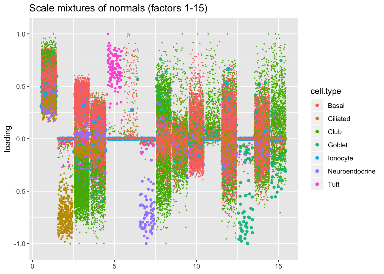
plot.factors(res$pn$fl, processed$cell.type, pn.order[16:30],
             title = "Point-normal priors (factors 16-30)")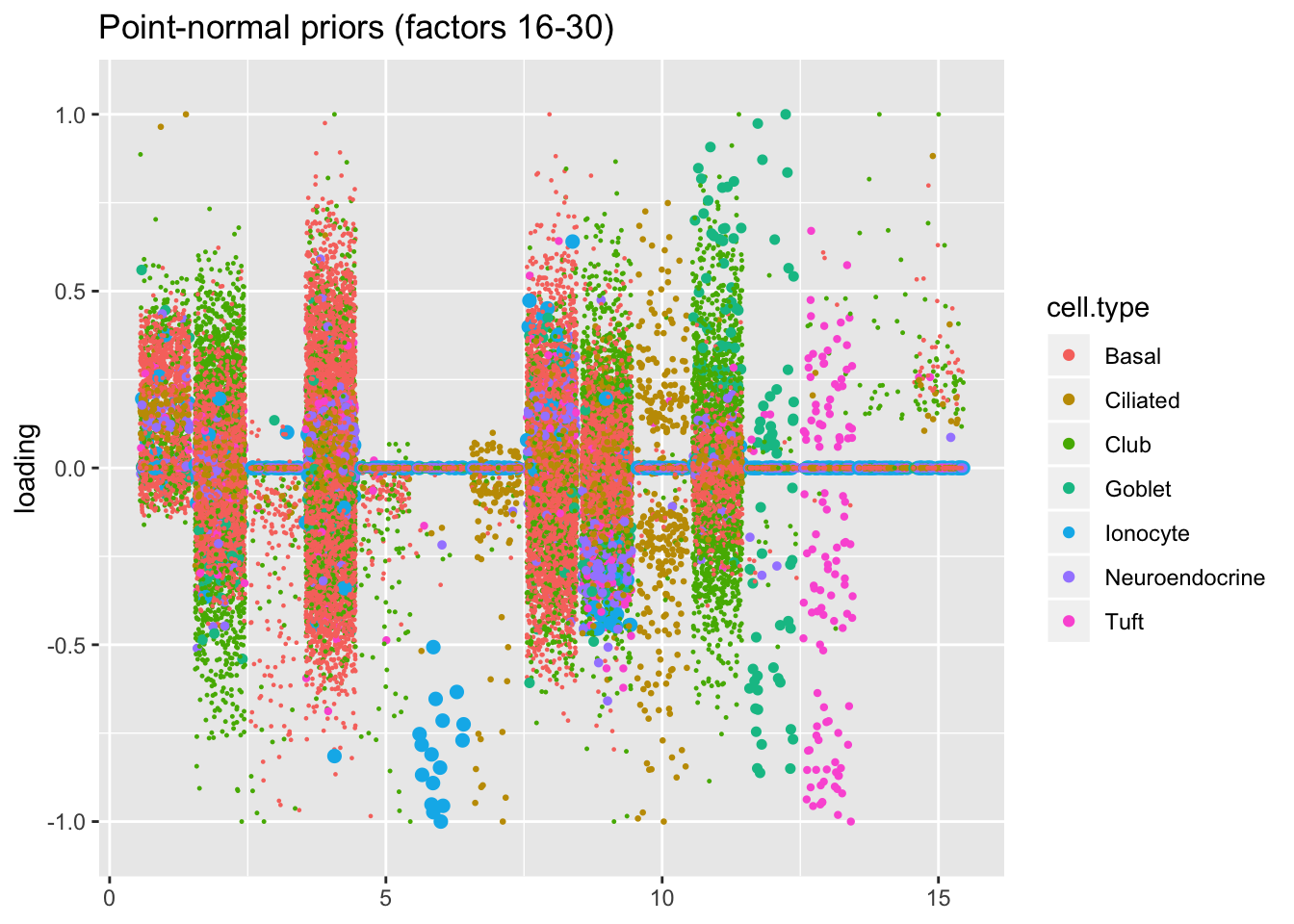
plot.factors(res$ash$fl, processed$cell.type, ash.order[16:30],
             title = "Scale mixtures of normals (factors 16-30)")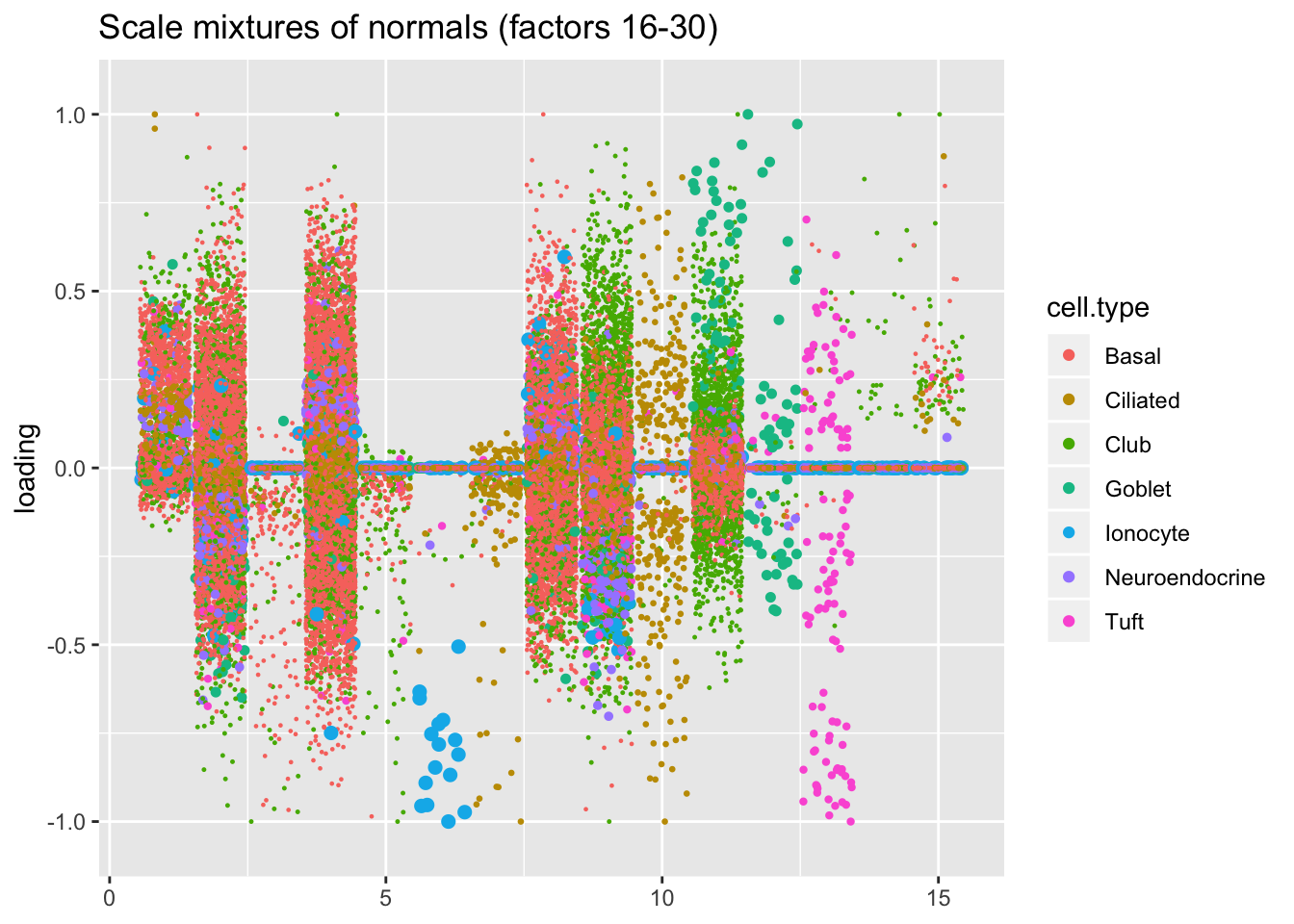
Results: semi-nonnegative factorizations
For ease of comparison, I only consider the semi-nonnegative fit that puts nonnegative priors on gene loadings. As above, I line up similar factors. I denote a semi-nonnegative factor as “similar” to a point-normal factor if the gene loadings are strongly correlated (\(r \ge 0.7\)) with either the positive or the negative component of the point-normal gene loadings. Thus there can be duplicates: factors 2 and 3 are represented by a single point-normal factor (one semi-nonnonegative factor is correlated with the positive component while another is correlated with the negative). The same is true of goblet factors 18 and 19.
In two cases, there are also duplicate semi-nonnegative factors: as it turns out, one of the semi-nonnegative tuft factors is similar to both point-normal tuft factors (factors 7 and 23 below). Point-normal hillock factors 6 and 12 are also matched by a single semi-nonnegative factor.
cor.thresh <- 0.7

pn.pos <- pmax(res$pn$fl$loadings.pm[[2]], 0)
pn.pos <- t(t(pn.pos) / apply(pn.pos, 2, function(x) sqrt(sum(x^2))))
pos.cor <- crossprod(res$snn.gene$fl$loadings.pm[[2]], pn.pos)

pn.neg <- -pmin(res$pn$fl$loadings.pm[[2]], 0)
pn.neg <- t(t(pn.neg) / apply(pn.neg, 2, function(x) sqrt(sum(x^2))))
pn.neg[, 1] <- 0
neg.cor <- crossprod(res$snn.gene$fl$loadings.pm[[2]], pn.neg)

is.cor <- (pmax(pos.cor, neg.cor) > cor.thresh)

pn.matched <- which(apply(is.cor, 2, any))
snn.matched <- unlist(lapply(pn.matched, function(x) which(is.cor[, x])))
# Duplicate factors where need be.
pn.matched <- rep(1:res$pn$fl$n.factors, times = apply(is.cor, 2, sum))

plot.factors(res$pn$fl, processed$cell.type,
             pn.matched, title = "Point-normal (matched factors)")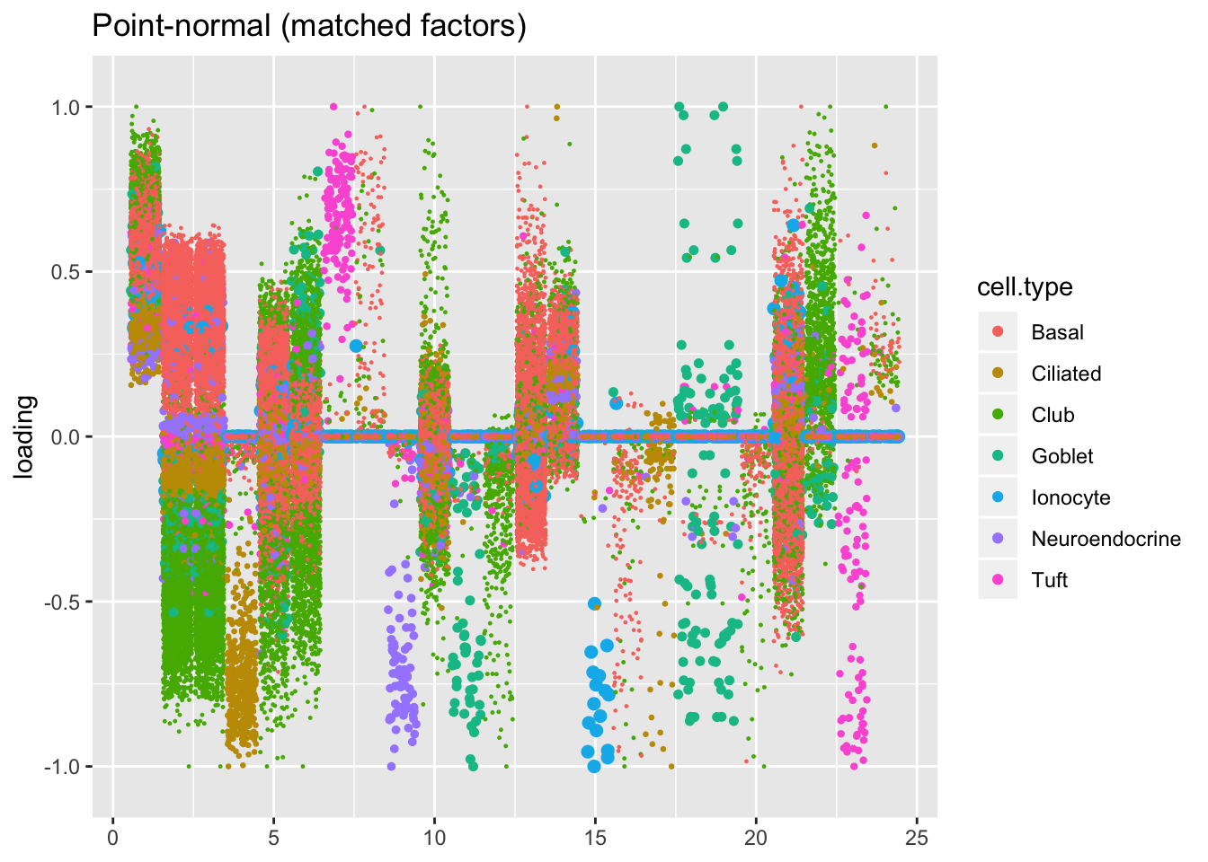
plot.factors(res$snn.gene$fl, processed$cell.type,
             snn.matched, title = "Semi-nonnegative (matched factors)")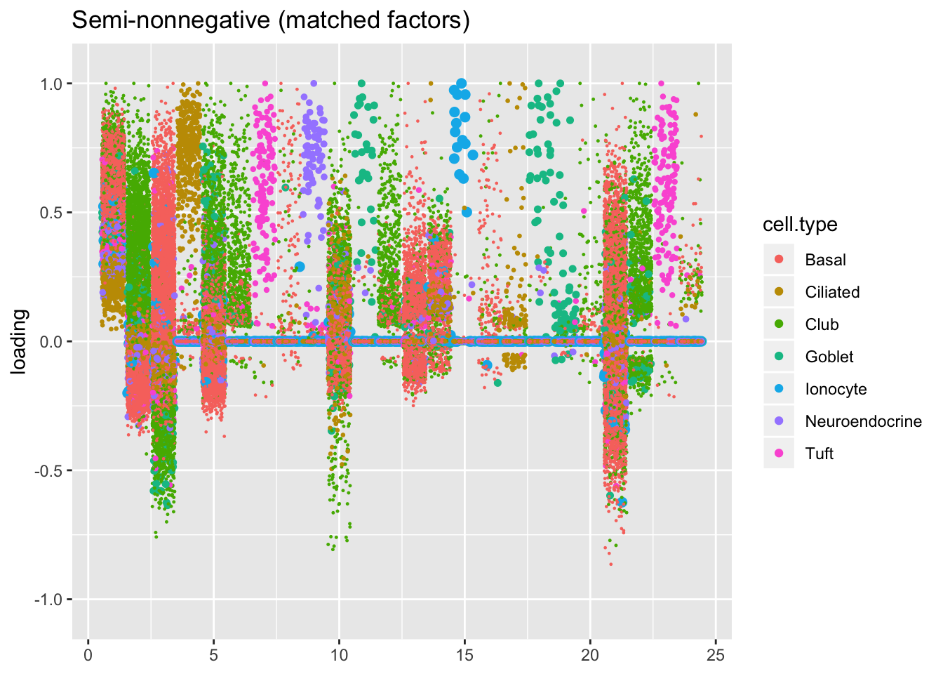
Next I plot the remaining “unmatched” factors. I’m not especially interested in trying to tease out the nuances in basal, club, and hillock factors that make up the majority of these factors. Worthy of note are:
Point-normal factor 7, which promises to identify a subpopulation of ciliated cells that is not represented by the semi-nonnegative fit. However, since the point-normal fit can, in theory, accommodate twice as many gene sets as the semi-nonnegative fit, it’s not terribly surprising that it yields at least one additional factor of interest.
The tuft factor (semi-nonnegative factor 9), which is not so much an additional factor as compensation for the fact that a single semi-nonnegative tuft factor does the work of two point-normal factors: see below.
snn.unmatched <- setdiff(1:res$snn.gene$fl$n.factors, snn.matched)
pn.unmatched <- setdiff(1:res$pn$fl$n.factors, pn.matched)

plot.factors(res$pn$fl, processed$cell.type,
             pn.unmatched, title = "Point-normal (unmatched factors)")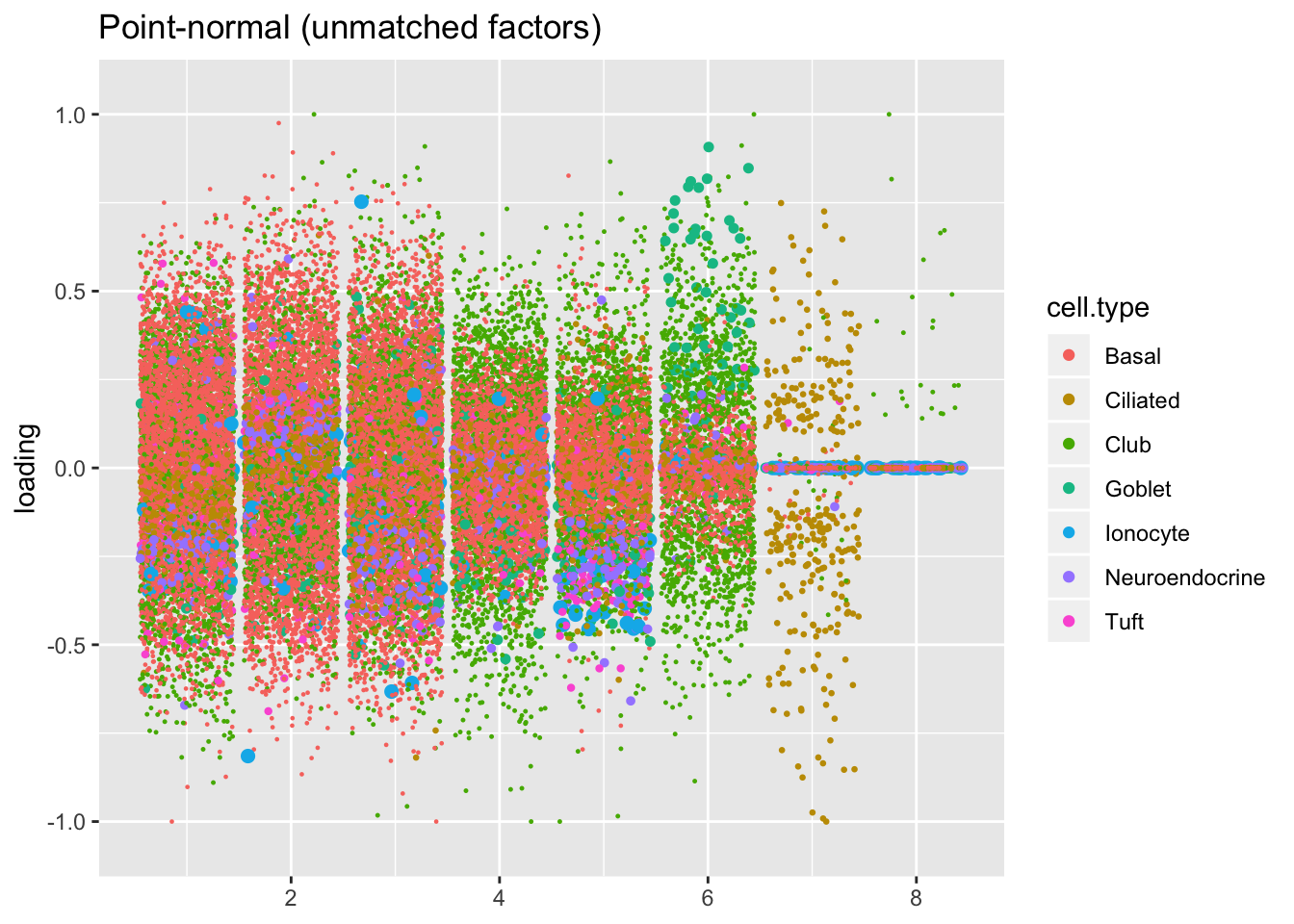
plot.factors(res$snn.gene$fl, processed$cell.type,
             snn.unmatched, title = "Semi-nonnegative (unmatched factors)")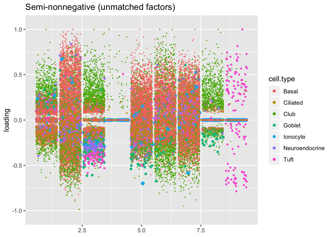
Results: tuft factors
Counting unnmatched semi-nonnegative factor 9, there are a total of two semi-nonnegative tuft factors, which is the same number of tuft factors as there are in the point-normal fit. And indeed, both fits similarly separate out tuft-1 and tuft-2 populations. The most obvious difference is that the point-normal fit gives us one factor (7) that identifies tuft cells and another factor (23) that discriminates between tuft-1 cells (positive loadings) and tuft-2 cells (negative loadings). In contrast, the semi-nonnegative fit gives us a factor that identifies tuft cells and a factor that further delimits tuft-1 cells; to get the tuft-2 gene set, one would need to “subtract” the tuft-1 loadings from the generic tuft loadings. So, although I claimed above that semi-nonnegative fits ought to be more interpretable, the point-normal fit is in fact easier to interpret here.
The relevant gene sets are plotted below. Genes that Montoro et al. identify as more highly expressed in tuft-1 cells are in blue, while genes that express more highly in tuft-2 cells are in red.
tuft1.genes <- c("Gnb3", "Gng13", "Itpr3", "Plcb2", "Gnat3", "Ovol3", "Commd1", "Cited2", "Atp1b1", "Fxyd6", "Pou2f3")
tuft2.genes <- c("Alox5ap", "Ptprc", "Spib", "Sox9", "Mgst3", "Gpx2", "Ly6e", "S100a11", "Cst3", "Cd24a", "B2m", "Dclk1", "Sdc4", "Il13ra1")
all.tuft.genes <- c("Il25", "Tslp", tuft1.genes, tuft2.genes)

gene.colors <- c(rep("black", 2),
                 rep("blue", length(tuft1.genes)),
                 rep("red", length(tuft2.genes)))

plot.one.factor(res$pn$fl, pn.matched[7], all.tuft.genes,
                "Point-normal, Factor 7",
                invert = FALSE, gene.colors = gene.colors)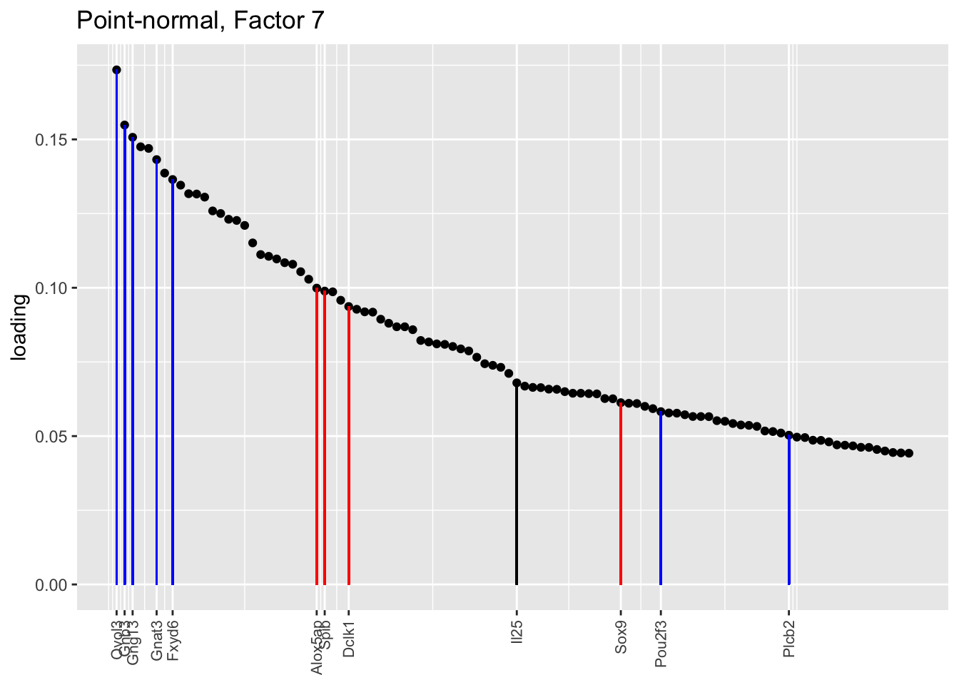
plot.one.factor(res$pn$fl, pn.matched[23], all.tuft.genes,
                "Point-normal, Factor 23 (positive component)",
                invert = FALSE, gene.colors = gene.colors)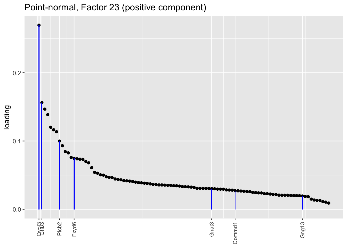
plot.one.factor(res$pn$fl, pn.matched[23], all.tuft.genes,
                "Point-normal, Factor 23 (negative component)",
                invert = TRUE, gene.colors = gene.colors)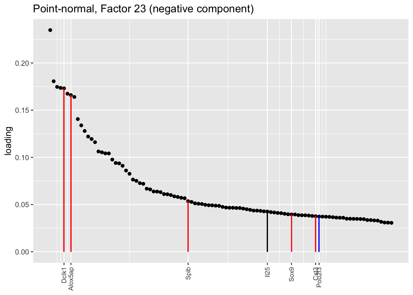
plot.one.factor(res$snn.gene$fl, snn.matched[7], all.tuft.genes,
                "Semi-nonnegative, Factor 7",
                invert = FALSE, gene.colors = gene.colors)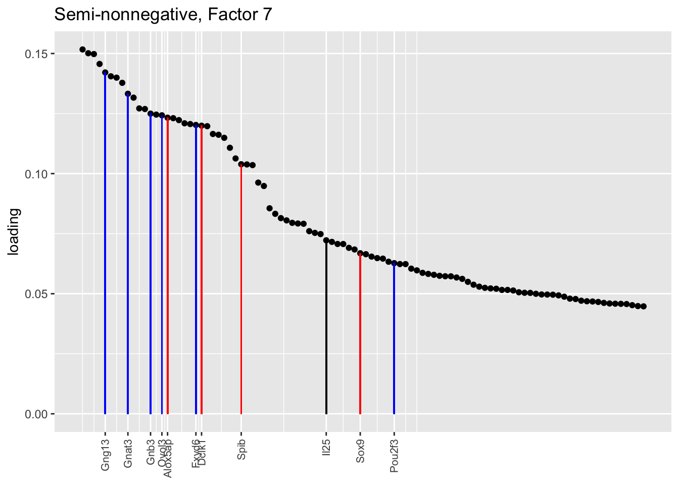
plot.one.factor(res$snn.gene$fl, snn.unmatched[9], all.tuft.genes,
                "Semi-nonnegative, Unmatched factor 9",
                invert = FALSE, gene.colors = gene.colors)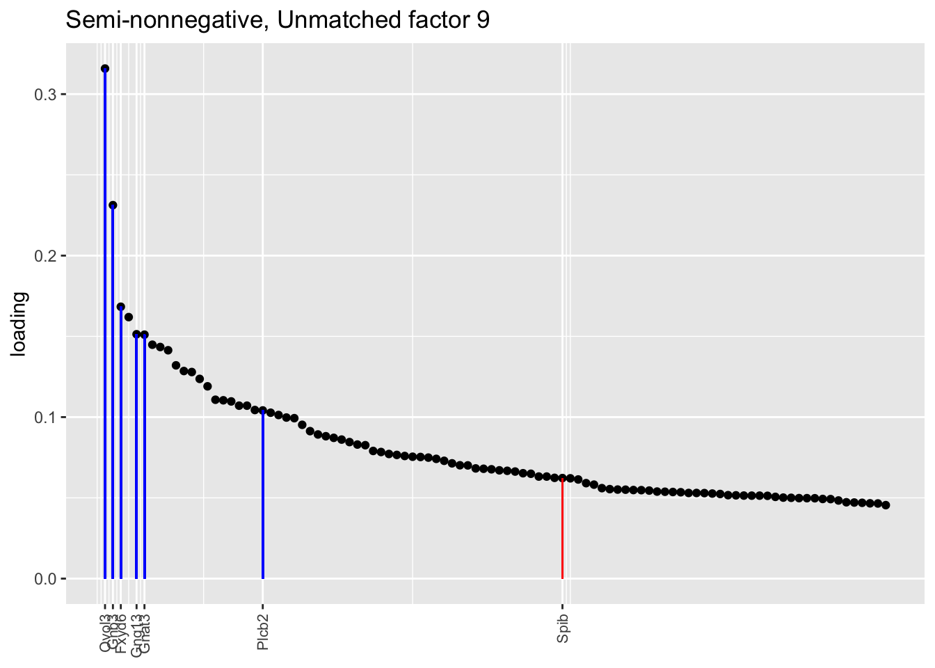
Some conclusions
I don’t think the semi-nonnegative fits are worth the trouble, at least with this dataset. They’re slow to fit and I’m not sure that they’re actually any more interpretable. If other datasets confirm that scale mixtures of normals can be fit nearly as quickly as point-normal priors, then I think that scale mixtures of normals might be the way to go.
# hillock.genes <- c("Krt13", "Krt4", "Ecm1", "S100a11", "Cldn3", "Lgals3", "Anxa1",
#                    "S100a6", "Upk3bl", "Aqp5", "Anxa2", "Crip1", "Gsto1", "Tppp3")
#
# snn.pve <- signif(res$snn.gene$fl$pve, digits = 2)
# plot.one.factor(res$snn.gene$fl, snn.matched[6], hillock.genes,
#                 paste0("Semi-nonnegative, Factor 6 (PVE: ",
#                        snn.pve[snn.matched[6]], ")"))
# plot.one.factor(res$snn.gene$fl, snn.matched[13], hillock.genes,
#                 paste0("Semi-nonnegative, Factor 13 (PVE: ",
#                        snn.pve[snn.matched[13]], ")"))
# plot.one.factor(res$snn.gene$fl, snn.unmatched[3], hillock.genes,
#                 paste0("Semi-nonnegative, Unmatched factor 3 (PVE: ",
#                        snn.pve[snn.unmatched[3]], ")"))
# plot.one.factor(res$snn.gene$fl, snn.unmatched[5], hillock.genes,
#                 paste0("Semi-nonnegative, Unmatched factor 5 (PVE: ",
#                        snn.pve[snn.unmatched[5]], ")"))
# plot.one.factor(res$snn.gene$fl, snn.unmatched[6], hillock.genes,
#                 paste0("Semi-nonnegative, Unmatched factor 6 (PVE: ",
#                        snn.pve[snn.unmatched[6]], ")"))
sessionInfo()R version 3.5.3 (2019-03-11)
Platform: x86_64-apple-darwin15.6.0 (64-bit)
Running under: macOS Mojave 10.14.6
Matrix products: default
BLAS: /Library/Frameworks/R.framework/Versions/3.5/Resources/lib/libRblas.0.dylib
LAPACK: /Library/Frameworks/R.framework/Versions/3.5/Resources/lib/libRlapack.dylib
locale:
[1] en_US.UTF-8/en_US.UTF-8/en_US.UTF-8/C/en_US.UTF-8/en_US.UTF-8
attached base packages:
[1] stats graphics grDevices utils datasets methods base
other attached packages:
[1] flashier_0.1.11 ggplot2_3.2.0 Matrix_1.2-15
loaded via a namespace (and not attached):
[1] Rcpp_1.0.1 plyr_1.8.4 highr_0.8
[4] compiler_3.5.3 pillar_1.3.1 git2r_0.25.2
[7] workflowr_1.2.0 iterators_1.0.10 tools_3.5.3
[10] digest_0.6.18 evaluate_0.13 tibble_2.1.1
[13] gtable_0.3.0 lattice_0.20-38 pkgconfig_2.0.2
[16] rlang_0.3.1 foreach_1.4.4 parallel_3.5.3
[19] yaml_2.2.0 ebnm_0.1-24 xfun_0.6
[22] withr_2.1.2 stringr_1.4.0 dplyr_0.8.0.1
[25] knitr_1.22 fs_1.2.7 rprojroot_1.3-2
[28] grid_3.5.3 tidyselect_0.2.5 glue_1.3.1
[31] R6_2.4.0 rmarkdown_1.12 mixsqp_0.1-119
[34] reshape2_1.4.3 ashr_2.2-38 purrr_0.3.2
[37] magrittr_1.5 whisker_0.3-2 MASS_7.3-51.1
[40] codetools_0.2-16 backports_1.1.3 scales_1.0.0
[43] htmltools_0.3.6 assertthat_0.2.1 colorspace_1.4-1
[46] labeling_0.3 stringi_1.4.3 pscl_1.5.2
[49] doParallel_1.0.14 lazyeval_0.2.2 munsell_0.5.0
[52] truncnorm_1.0-8 SQUAREM_2017.10-1 crayon_1.3.4