Results
2021-June-07
Last updated: 2021-07-14
Checks: 7 0
Knit directory: implementGMSinCassava/
This reproducible R Markdown analysis was created with workflowr (version 1.6.2). The Checks tab describes the reproducibility checks that were applied when the results were created. The Past versions tab lists the development history.
Great! Since the R Markdown file has been committed to the Git repository, you know the exact version of the code that produced these results.
Great job! The global environment was empty. Objects defined in the global environment can affect the analysis in your R Markdown file in unknown ways. For reproduciblity it’s best to always run the code in an empty environment.
The command set.seed(20210504) was run prior to running the code in the R Markdown file. Setting a seed ensures that any results that rely on randomness, e.g. subsampling or permutations, are reproducible.
Great job! Recording the operating system, R version, and package versions is critical for reproducibility.
Nice! There were no cached chunks for this analysis, so you can be confident that you successfully produced the results during this run.
Great job! Using relative paths to the files within your workflowr project makes it easier to run your code on other machines.
Great! You are using Git for version control. Tracking code development and connecting the code version to the results is critical for reproducibility.
The results in this page were generated with repository version 772750a. See the Past versions tab to see a history of the changes made to the R Markdown and HTML files.
Note that you need to be careful to ensure that all relevant files for the analysis have been committed to Git prior to generating the results (you can use wflow_publish or wflow_git_commit). workflowr only checks the R Markdown file, but you know if there are other scripts or data files that it depends on. Below is the status of the Git repository when the results were generated:
Ignored files:
    Ignored:    .DS_Store
    Ignored:    .Rhistory
    Ignored:    .Rproj.user/
    Ignored:    analysis/accuracies.png
    Ignored:    analysis/fig2.png
    Ignored:    analysis/fig3.png
    Ignored:    analysis/fig4.png
    Ignored:    code/.DS_Store
    Ignored:    data/.DS_Store

Untracked files:
    Untracked:  accuracies.png
    Untracked:  analysis/docs/
    Untracked:  analysis/inputsForSimulation.Rmd
    Untracked:  analysis/speedUpPredCrossVar.Rmd
    Untracked:  code/AlphaAssign-Python/
    Untracked:  code/calcGameticLD.cpp
    Untracked:  code/col_sums.cpp
    Untracked:  code/convertDart2vcf.R
    Untracked:  code/helloworld.cpp
    Untracked:  code/imputationFunctions.R
    Untracked:  code/matmult.cpp
    Untracked:  code/misc.cpp
    Untracked:  code/test.cpp
    Untracked:  data/CassavaGeneticMap/
    Untracked:  data/DatabaseDownload_2021May04/
    Untracked:  data/GBSdataMasterList_31818.csv
    Untracked:  data/IITA_GBStoPhenoMaster_33018.csv
    Untracked:  data/NRCRI_GBStoPhenoMaster_40318.csv
    Untracked:  data/PedigreeGeneticGainCycleTime_aafolabi_01122020.xls
    Untracked:  data/blups_forCrossVal.rds
    Untracked:  data/chr1_RefPanelAndGSprogeny_ReadyForGP_72719.fam
    Untracked:  data/dosages_IITA_filtered_2021May13.rds
    Untracked:  data/genmap_2021May13.rds
    Untracked:  data/haps_IITA_filtered_2021May13.rds
    Untracked:  data/recombFreqMat_1minus2c_2021May13.rds
    Untracked:  fig2.png
    Untracked:  fig3.png
    Untracked:  figure/
    Untracked:  output/IITA_CleanedTrialData_2021May10.rds
    Untracked:  output/IITA_ExptDesignsDetected_2021May10.rds
    Untracked:  output/IITA_blupsForModelTraining_twostage_asreml_2021May10.rds
    Untracked:  output/IITA_trials_NOT_identifiable.csv
    Untracked:  output/crossValPredsA.rds
    Untracked:  output/crossValPredsAD.rds
    Untracked:  output/cvAD_5rep5fold_markerEffects.rds
    Untracked:  output/cvAD_5rep5fold_meanPredAccuracy.rds
    Untracked:  output/cvAD_5rep5fold_parentfolds.rds
    Untracked:  output/cvAD_5rep5fold_predMeans.rds
    Untracked:  output/cvAD_5rep5fold_predVars.rds
    Untracked:  output/cvAD_5rep5fold_varPredAccuracy.rds
    Untracked:  output/cvDirDom_5rep5fold_markerEffects.rds
    Untracked:  output/cvDirDom_5rep5fold_meanPredAccuracy.rds
    Untracked:  output/cvDirDom_5rep5fold_parentfolds.rds
    Untracked:  output/cvDirDom_5rep5fold_predMeans.rds
    Untracked:  output/cvDirDom_5rep5fold_predVars.rds
    Untracked:  output/cvDirDom_5rep5fold_varPredAccuracy.rds
    Untracked:  output/cvMeanPredAccuracyA.rds
    Untracked:  output/cvMeanPredAccuracyAD.rds
    Untracked:  output/cvPredMeansA.rds
    Untracked:  output/cvPredMeansAD.rds
    Untracked:  output/cvVarPredAccuracyA.rds
    Untracked:  output/cvVarPredAccuracyAD.rds
    Untracked:  output/estimateSelectionError.rds
    Untracked:  output/genomicPredictions_ModelAD.rds
    Untracked:  output/genomicPredictions_ModelDirDom.rds
    Untracked:  output/kinship_A_IITA_2021May13.rds
    Untracked:  output/kinship_D_IITA_2021May13.rds
    Untracked:  output/markEffsTest.rds
    Untracked:  output/markerEffects.rds
    Untracked:  output/markerEffectsA.rds
    Untracked:  output/markerEffectsAD.rds
    Untracked:  output/maxNOHAV_byStudy.csv
    Untracked:  output/obsCrossMeansAndVars.rds
    Untracked:  output/parentfolds.rds
    Untracked:  output/ped2check_genome.rds
    Untracked:  output/ped2genos.txt
    Untracked:  output/pednames2keep.txt
    Untracked:  output/pednames_Prune100_25_pt25.log
    Untracked:  output/pednames_Prune100_25_pt25.nosex
    Untracked:  output/pednames_Prune100_25_pt25.prune.in
    Untracked:  output/pednames_Prune100_25_pt25.prune.out
    Untracked:  output/potential_dams.txt
    Untracked:  output/potential_sires.txt
    Untracked:  output/predVarTest.rds
    Untracked:  output/samples2keep_IITA_2021May13.txt
    Untracked:  output/samples2keep_IITA_MAFpt01_prune50_25_pt98.log
    Untracked:  output/samples2keep_IITA_MAFpt01_prune50_25_pt98.nosex
    Untracked:  output/samples2keep_IITA_MAFpt01_prune50_25_pt98.prune.in
    Untracked:  output/samples2keep_IITA_MAFpt01_prune50_25_pt98.prune.out
    Untracked:  output/verified_ped.txt
Note that any generated files, e.g. HTML, png, CSS, etc., are not included in this status report because it is ok for generated content to have uncommitted changes.
These are the previous versions of the repository in which changes were made to the R Markdown (analysis/07-Results.Rmd) and HTML (docs/07-Results.html) files. If you’ve configured a remote Git repository (see ?wflow_git_remote), click on the hyperlinks in the table below to view the files as they were in that past version.
| File | Version | Author | Date | Message |
|---|---|---|---|---|
| Rmd | 772750a | wolfemd | 2021-07-14 | DirDom model and selection index calc fully integrated functions. |
Raw data
Summary of the number of unique plots, locations, years, etc. in the cleaned plot-basis data. See here for details..
library(tidyverse); library(magrittr); library(ragg)
rawdata<-readRDS(file=here::here("output","IITA_ExptDesignsDetected_2021May10.rds"))
rawdata %>%
  summarise(Nplots=nrow(.),
            across(c(locationName,studyYear,studyName,TrialType,GID), ~length(unique(.)),.names = "N_{.col}")) %>%
  rmarkdown::paged_table()
This is not the same number of clones as are expected to be genotyped-and-phenotyped.
Break down the plots based on the trial design and TrialType (really a grouping of the population that is breeding program specific), captured by two logical variables, CompleteBlocks and IncompleteBlocks.
rawdata %>%
  count(TrialType,CompleteBlocks,IncompleteBlocks) %>%
  spread(TrialType,n) %>%
  rmarkdown::paged_table()
Next, look at breakdown of plots by TrialType (rows) and locations (columns):
rawdata %>%
  count(locationName,TrialType) %>%
  spread(locationName,n) %>%
rmarkdown::paged_table()traits<-c("MCMDS","DM","PLTHT","BRNHT1","BRLVLS","HI",
"logDYLD", # <-- logDYLD now included.
"logFYLD","logTOPYLD","logRTNO","TCHART","LCHROMO","ACHROMO","BCHROMO")
rawdata %>%
select(locationName,studyYear,studyName,TrialType,any_of(traits)) %>%
pivot_longer(cols = any_of(traits), values_to = "Value", names_to = "Trait") %>%
ggplot(.,aes(x=Value,fill=Trait)) + geom_histogram() + facet_wrap(~Trait, scales='free') +
theme_bw() + scale_fill_viridis_d() +
labs(title = "Distribution of Raw Phenotypic Values")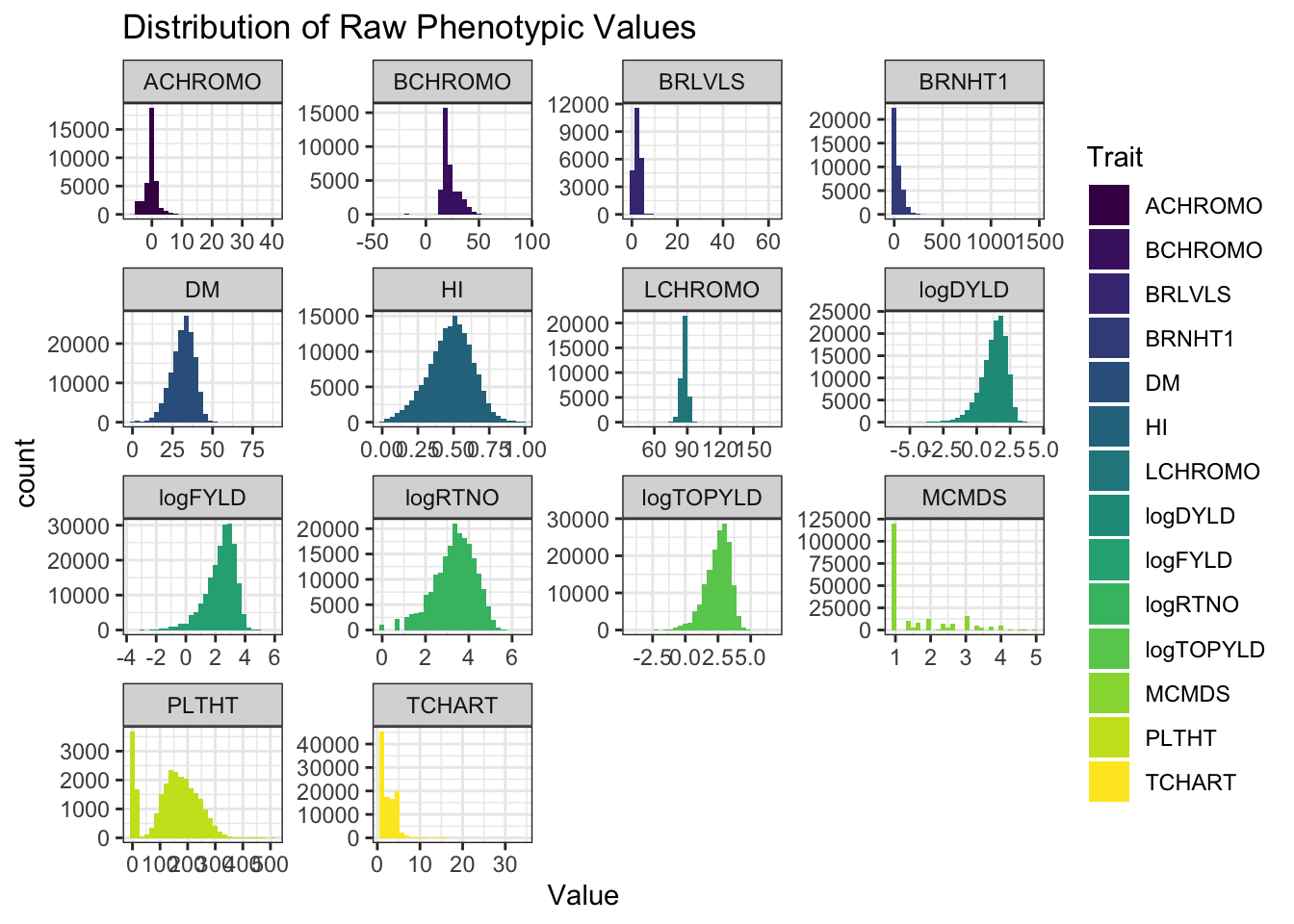 How many genotyped-and-phenotyped clones?
rawdata %>%
  select(locationName,studyYear,studyName,TrialType,germplasmName,FullSampleName,GID,any_of(traits)) %>%
  pivot_longer(cols = any_of(traits), values_to = "Value", names_to = "Trait") %>%
  filter(!is.na(Value),!is.na(FullSampleName)) %>%
  distinct(germplasmName,FullSampleName,GID) %>%
  rmarkdown::paged_table()
There are 8149 genotyped-and-phenotyped clones!
BLUPs
These are the BLUPs combining data for each clone across trials/locations without genomic information, used as input for genomic prediction downstream.
blups<-readRDS(file=here::here("data","blups_forCrossVal.rds"))
gidWithBLUPs<-blups %>% select(Trait,blups) %>% unnest(blups) %$% unique(GID)
rawdata %>%
  select(observationUnitDbId,GID,any_of(blups$Trait)) %>%
  pivot_longer(cols = any_of(blups$Trait),
               names_to = "Trait",
               values_to = "Value",values_drop_na = T) %>%
  filter(GID %in% gidWithBLUPs) %>%
  group_by(Trait) %>%
  summarize(Nplots=n()) %>%
  ungroup() %>%
  left_join(blups %>%
              mutate(Nclones=map_dbl(blups,~nrow(.)),
                     avgREL=map_dbl(blups,~mean(.$REL)),
                     Vg=map_dbl(varcomp,~.["GID!GID.var","component"]),
                     Ve=map_dbl(varcomp,~.["R!variance","component"]),
                     H2=Vg/(Vg+Ve)) %>%
              select(-blups,-varcomp)) %>%
  mutate(across(is.numeric,~round(.,3))) %>% arrange(desc(H2)) %>%
  rmarkdown::paged_table()
blups %>%
select(Trait,blups) %>%
unnest(blups) %>%
ggplot(.,aes(x=drgBLUP,fill=Trait)) + geom_histogram() + facet_wrap(~Trait, scales='free') +
theme_bw() + scale_fill_viridis_d() + theme(legend.position = 'none') +
labs(title = "Distribution of de-regressed BLUP Values")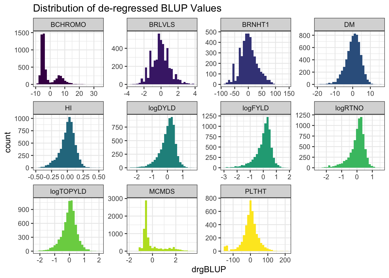
blups %>%
select(Trait,blups) %>%
unnest(blups) %>%
ggplot(.,aes(x=Trait,y=REL,fill=Trait)) + geom_boxplot(notch=T) + #facet_wrap(~Trait, scales='free') +
theme_bw() + scale_fill_viridis_d() +
theme(axis.text.x = element_text(angle=90),
legend.position = 'none') +
labs(title = "Distribution of BLUP Reliabilities")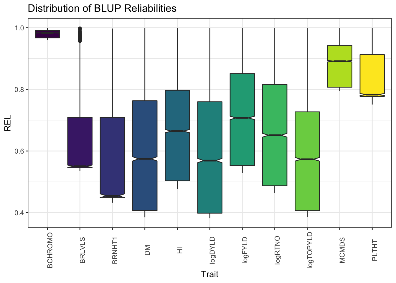 # Marker density and distribution
library(tidyverse); library(magrittr);
snps<-readRDS(file=here::here("data","dosages_IITA_filtered_2021May13.rds"))
mrks<-colnames(snps) %>%
  tibble(SNP_ID=.) %>%
  separate(SNP_ID,c("Chr","Pos","Allele"),"_") %>%
  mutate(Chr=as.integer(gsub("S","",Chr)),
         Pos=as.numeric(Pos))
mrks %>%
  ggplot(.,aes(x=Pos,fill=as.character(Chr))) + geom_histogram() +
  facet_wrap(~Chr,scales = 'free') + theme_bw() +
  scale_fill_viridis_d() + theme(legend.position = 'none',
                                 axis.text.x = element_text(angle=90))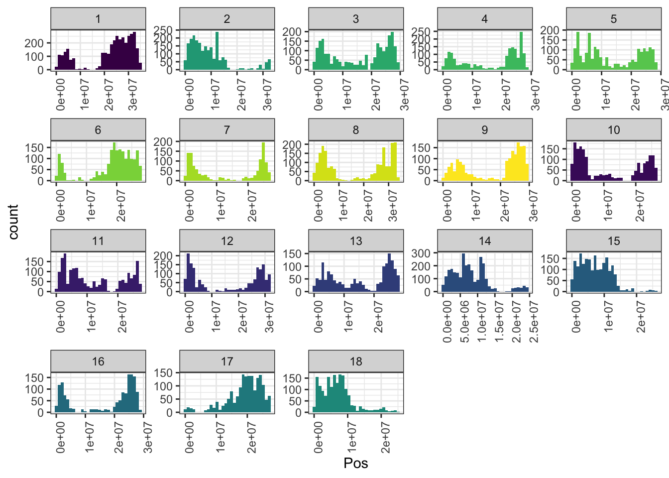
mrks %>% count(Chr) %>% rmarkdown::paged_table()Pedigree
Summarize the pedigree and the verification results described here.
library(tidyverse); library(magrittr);
ped2check_genome<-readRDS(file=here::here("output","ped2check_genome.rds"))
ped2check_genome %<>%
  select(IID1,IID2,Z0,Z1,Z2,PI_HAT)
ped2check<-read.table(file=here::here("output","ped2genos.txt"),
                      header = F, stringsAsFactors = F) %>%
  rename(FullSampleName=V1,DamID=V2,SireID=V3)
ped2check %<>%
  select(FullSampleName,DamID,SireID) %>%
  inner_join(ped2check_genome %>%
               rename(FullSampleName=IID1,DamID=IID2) %>%
               bind_rows(ped2check_genome %>%
                           rename(FullSampleName=IID2,DamID=IID1))) %>%
  distinct %>%
  mutate(FemaleParent=case_when(Z0<0.32 & Z1>0.67~"Confirm",
                                       SireID==DamID & PI_HAT>0.6 & Z0<0.3 & Z2>0.32~"Confirm",
                                       TRUE~"Reject")) %>%
  select(-Z0,-Z1,-Z2,-PI_HAT) %>%
  inner_join(ped2check_genome %>%
               rename(FullSampleName=IID1,SireID=IID2) %>%
               bind_rows(ped2check_genome %>%
                           rename(FullSampleName=IID2,SireID=IID1))) %>%
  distinct %>%
  mutate(MaleParent=case_when(Z0<0.32 & Z1>0.67~"Confirm",
                                       SireID==DamID & PI_HAT>0.6 & Z0<0.3 & Z2>0.32~"Confirm",
                                       TRUE~"Reject")) %>%
  select(-Z0,-Z1,-Z2,-PI_HAT)
rm(ped2check_genome)

ped2check %<>%
  mutate(Cohort=NA,
         Cohort=ifelse(grepl("TMS18",FullSampleName,ignore.case = T),"TMS18",
                       ifelse(grepl("TMS15",FullSampleName,ignore.case = T),"TMS15",
                              ifelse(grepl("TMS14",FullSampleName,ignore.case = T),"TMS14",
                                     ifelse(grepl("TMS13|2013_",FullSampleName,ignore.case = T),"TMS13","GGetc")))))
Proportion of accessions with male, female or both parents in pedigree confirm-vs-rejected?
ped2check %>%
  count(FemaleParent,MaleParent) %>%
  mutate(Prop=round(n/sum(n),2))
FemaleParent MaleParent n Prop
1 Confirm Confirm 4259 0.77
2 Confirm Reject 563 0.10
3 Reject Confirm 382 0.07
4 Reject Reject 313 0.06Proportion of accessions within each Cohort with pedigree records confirmed-vs-rejected?
ped2check %>%
  count(Cohort,FemaleParent,MaleParent) %>%
  spread(Cohort,n) %>%
  mutate(across(is.numeric,~round(./sum(.),2))) %>%
  rmarkdown::paged_table()
Use only fully-confirmed families / trios. Remove any without both parents confirmed.
ped<-read.table(here::here("output","verified_ped.txt"),
                header = T, stringsAsFactors = F) %>%
  mutate(Cohort=NA,
         Cohort=ifelse(grepl("TMS18",FullSampleName,ignore.case = T),"TMS18",
                       ifelse(grepl("TMS15",FullSampleName,ignore.case = T),"TMS15",
                              ifelse(grepl("TMS14",FullSampleName,ignore.case = T),"TMS14",
                                     ifelse(grepl("TMS13|2013_",FullSampleName,ignore.case = T),"TMS13","GGetc")))))
Summary of family sizes
ped %>%
  count(SireID,DamID) %$% summary(n)
Min. 1st Qu. Median Mean 3rd Qu. Max.
1.00 1.00 3.00 5.85 8.00 77.00 ped %>% nrow(.) # 4259 pedigree entries[1] 4259ped %>%
count(Cohort,name = "Number of Verified Pedigree Entries") Cohort Number of Verified Pedigree Entries
1 GGetc 18
2 TMS13 1786
3 TMS14 1302
4 TMS15 589
5 TMS18 564ped %>%
distinct(Cohort,SireID,DamID) %>%
count(Cohort,name = "Number of Families per Cohort") Cohort Number of Families per Cohort
1 GGetc 16
2 TMS13 120
3 TMS14 233
4 TMS15 197
5 TMS18 164730 families. Mean size 5.85, range 1-77.
Parent-wise Cross-validation
parentfolds<-readRDS(file=here::here("output","parentfolds.rds"))
summarized_parentfolds<-parentfolds %>%
  mutate(Ntestparents=map_dbl(testparents,length),
         Ntrainset=map_dbl(trainset,length),
         Ntestset=map_dbl(testset,length),
         NcrossesToPredict=map_dbl(CrossesToPredict,nrow)) %>%
  select(Repeat,Fold,starts_with("N"))
summarized_parentfolds %>%
  rmarkdown::paged_table()
summarized_parentfolds %>% summarize(across(is.numeric,median,.names = "median{.col}"))# A tibble: 1 x 4
medianNtestparents medianNtrainset medianNtestset medianNcrossesToPredict
<dbl> <dbl> <dbl> <dbl>
1 55 2053 2125 195Selection index weights
c(logFYLD=20,
  HI=10,
  DM=15,
  MCMDS=-10,
  logRTNO=12,
  logDYLD=20,
  logTOPYLD=15,
  PLTHT=10)
logFYLD HI DM MCMDS logRTNO logDYLD logTOPYLD PLTHT
20 10 15 -10 12 20 15 10 Prediction accuracy
- Check prediction accuracy: Evaluate prediction accuracy with cross-validation.
Selection Index Accuracy
Selection index weights
# SELECTION INDEX WEIGHTS
## from IYR+IK
## note that not ALL predicted traits are on index
SIwts<-c(logFYLD=20,
         HI=10,
         DM=15,
         MCMDS=-10,
         logRTNO=12,
         logDYLD=20,
         logTOPYLD=15,
         PLTHT=10)
SIwts
logFYLD HI DM MCMDS logRTNO logDYLD logTOPYLD PLTHT
20 10 15 -10 12 20 15 10 library(ggdist)
accuracy_ad<-readRDS(here::here("output","cvAD_5rep5fold_predAccuracy.rds"))
accuracy_dirdom<-readRDS(here::here("output","cvDirDom_5rep5fold_predAccuracy.rds"))
accuracy<-accuracy_ad$meanPredAccuracy %>%
bind_rows(accuracy_dirdom$meanPredAccuracy) %>%
filter(Trait=="SELIND") %>%
mutate(VarComp=gsub("Mean","",predOf),
predOf="Mean") %>%
bind_rows(accuracy_ad$varPredAccuracy %>%
bind_rows(accuracy_dirdom$varPredAccuracy) %>%
filter(Trait1=="SELIND") %>%
rename(Trait=Trait1) %>%
select(-Trait2) %>%
mutate(VarComp=gsub("Var","",predOf),
predOf="Var")) %>%
select(-predVSobs)
colors<-viridis::viridis(4)[1:2]accuracy %>%
mutate(predOf=factor(predOf,levels=c("Mean","Var")),
VarComp=factor(VarComp,levels=c("BV","TGV"))) %>%
ggplot(.,aes(x=VarComp,y=AccuracyEst,fill=VarComp)) +
ggdist::stat_halfeye(adjust=0.5,.width = 0,fill='gray',width=0.75) +
geom_boxplot(width=0.12,notch = TRUE) +
ggdist::stat_dots(side = "left",justification = 1.1,
binwidth = 0.03,dotsize=0.6) +
theme_bw() +
scale_fill_manual(values = colors) +
geom_hline(yintercept = 0, color='black', size=0.9) +
theme(axis.text.x = element_blank(),
axis.title.x = element_blank(),
strip.background = element_blank(),
panel.grid.major = element_blank(),
panel.grid.minor = element_blank(),
axis.title = element_text(face='bold',color = 'black'),
strip.text.x = element_text(face='bold',color='black',size=14),
axis.text.y = element_text(face = 'bold',color='black'),
legend.text = element_text(face='bold'),
legend.position = 'bottom') +
facet_grid(predOf~modelType,scales = 'free') +
#facet_wrap(~predOf+modelType,scales = 'free_y',nrow=1) +
labs(title="Selection Index Prediction Accuracy") +
coord_cartesian(xlim = c(1.2, NA))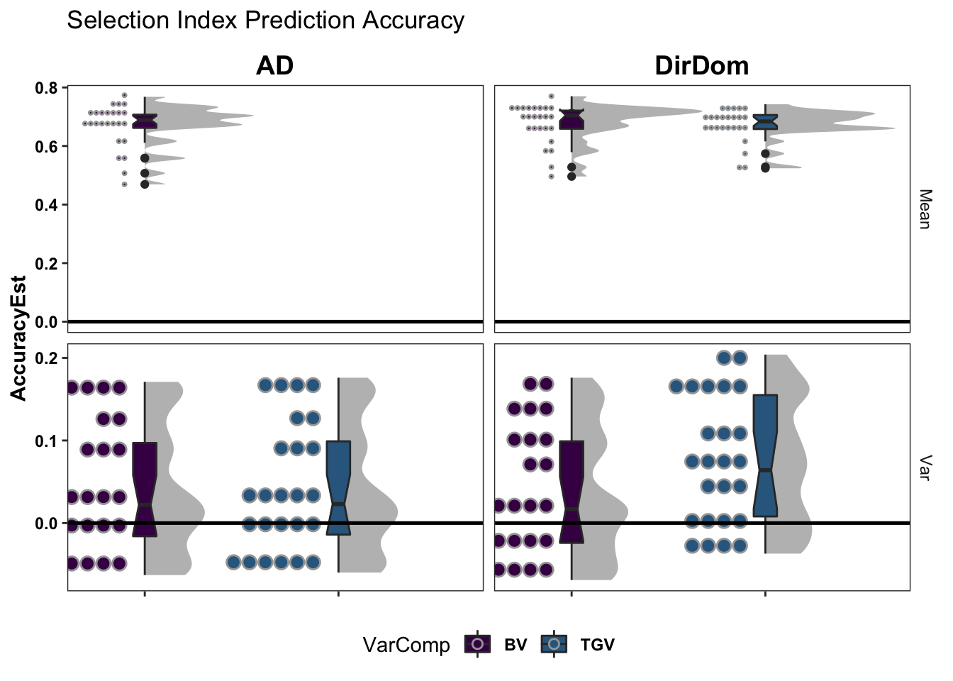
Accuracy predicting cross-means
accuracy_ad$meanPredAccuracy %>%
  bind_rows(accuracy_dirdom$meanPredAccuracy) %>%
  select(-predVSobs) %>%
  mutate(Trait=factor(Trait,levels=c("SELIND",blups$Trait)),
         predOf=factor(paste0(predOf,"_",modelType),levels=c("MeanBV_AD","MeanTGV_AD","MeanBV_DirDom","MeanTGV_DirDom"))) %>%
  ggplot(.,aes(x=predOf,y=AccuracyEst,fill=predOf,color=modelType)) +
  geom_boxplot(width=0.4,notch = TRUE, color='gray40') +
  ggdist::stat_dots(side = "left", justification = 1.3,
                    binwidth = 0.03,dotsize=0.5,layout="swarm") +
  scale_fill_manual(values = viridis::viridis(4)[1:4]) +
  scale_color_manual(values = viridis::viridis(4)[1:4]) +
  geom_hline(yintercept = 0, color='black', size=0.8) +
  facet_grid(.~Trait) +
  labs(title="Accuracy predicting cross-means") +
  theme_bw() +
  theme(axis.text.x = element_blank(),
        axis.title.x = element_blank(),
        strip.background = element_blank(),
        panel.grid.major = element_blank(),
        panel.grid.minor = element_blank(),
        axis.text.y = element_text(face='bold'),
        strip.text.x = element_text(face='bold'),
        legend.position='bottom',
        legend.text = element_text(face='bold'),
        panel.spacing = unit(0.05, "lines"))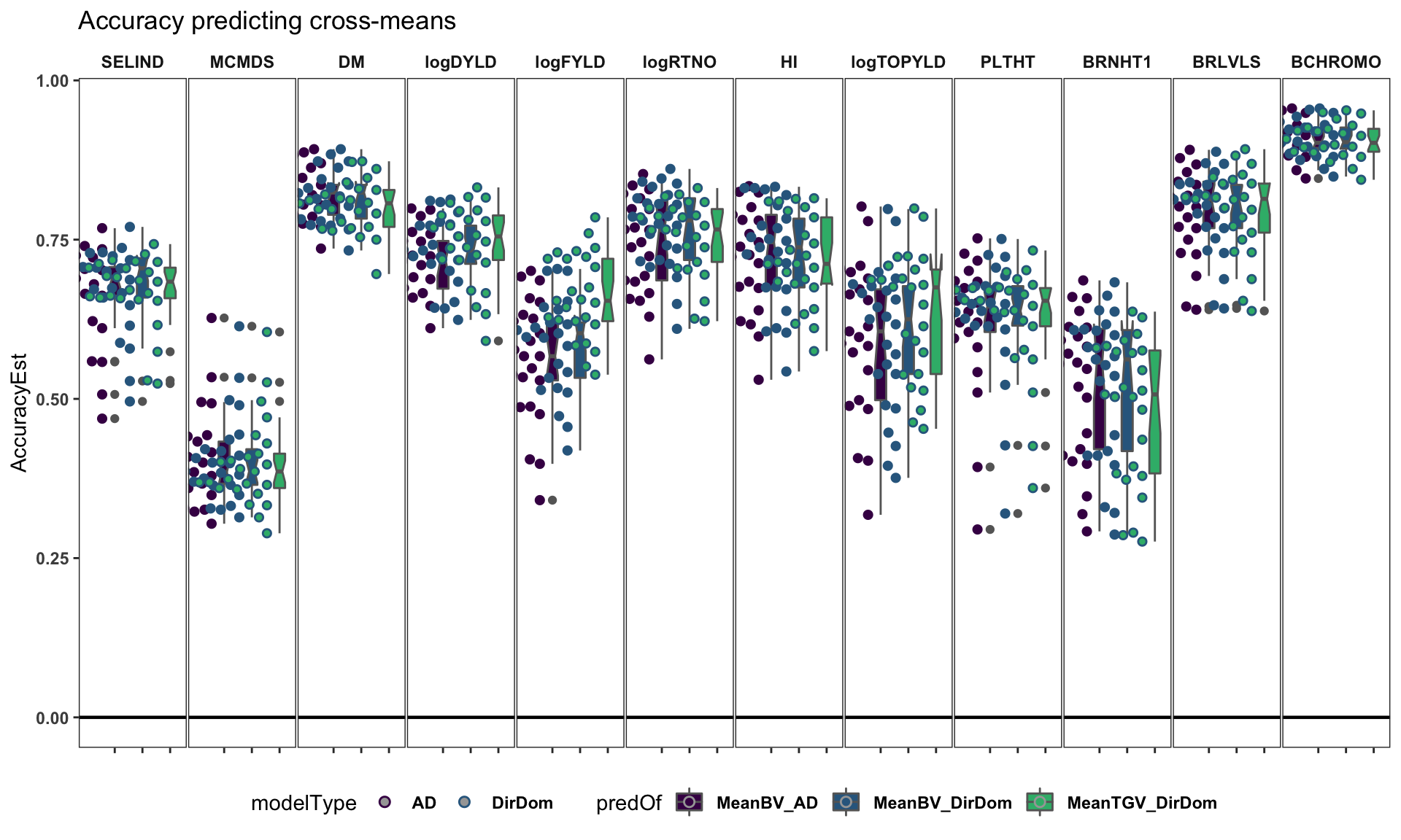
Accuracy predicting variance params
accuracy_ad$varPredAccuracy %>%
  bind_rows(accuracy_dirdom$varPredAccuracy) %>%
  select(-predVSobs) %>%
  filter(Trait1==Trait2) %>%
  mutate(Trait1=factor(Trait1,levels=c("SELIND",blups$Trait)),
         predOf=factor(paste0(predOf,"_",modelType),
                       levels=c("VarBV_AD","VarTGV_AD",
                                "VarBV_DirDom","VarTGV_DirDom"))) %>%
  ggplot(.,aes(x=predOf,y=AccuracyEst,fill=predOf,color=modelType)) +
  geom_boxplot(width=0.4,notch = TRUE,color='gray40') +
  ggdist::stat_dots(side = "left", justification = 1.3,layout='swarm',
                    binwidth = 0.03,dotsize=0.4) +
  scale_fill_manual(values = viridis::viridis(4)[1:4]) +
  scale_color_manual(values = viridis::viridis(4)[1:4]) +
  geom_hline(yintercept = 0, color='black', size=0.8) +
  facet_grid(.~Trait1) +
  labs(title="Accuracy predicting cross-variances") +
  theme_bw() +
  theme(axis.text.x = element_blank(),
        axis.title.x = element_blank(),
        strip.background = element_blank(),
        panel.grid.major = element_blank(),
        panel.grid.minor = element_blank(),
        axis.text.y = element_text(face='bold'),
        strip.text.x = element_text(face='bold'),
        legend.position='bottom',
        legend.text = element_text(face='bold'),
        panel.spacing = unit(0.05, "lines"))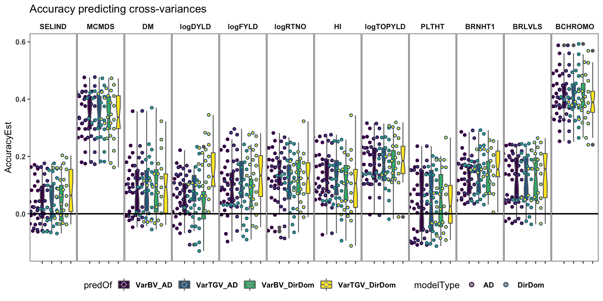
accuracy_ad$varPredAccuracy %>%
  bind_rows(accuracy_dirdom$varPredAccuracy) %>%
  select(-predVSobs) %>%
  filter(Trait1!="SELIND",Trait2!="SELIND",
         Trait1!=Trait2) %>%
  mutate(#Trait1=factor(Trait1,levels=c("SELIND",blups$Trait)),
         #Trait2=factor(Trait2,levels=c("SELIND",blups$Trait)),
         Trait1=factor(Trait1,levels=c(blups$Trait)),
         Trait2=factor(Trait2,levels=c(blups$Trait)),
         predOf=factor(paste0(predOf,"_",modelType),
                       levels=c("VarBV_AD","VarTGV_AD",
                                "VarBV_DirDom","VarTGV_DirDom"))) %>%
  ggplot(.,aes(x=predOf,y=AccuracyEst,fill=predOf,color=modelType)) +
  geom_boxplot(notch = TRUE) +
  scale_fill_manual(values = viridis::viridis(4)[1:4]) +
  scale_color_manual(values = viridis::viridis(4)[1:4]) +
  geom_hline(yintercept = 0, color='gray40', size=0.6) +
  facet_wrap(~Trait1+Trait2,nrow=5) +
  labs(title="Accuracy predicting cross-covariances") +
  theme_bw() +
  theme(axis.text.x = element_blank(),
        axis.title.x = element_blank(),
        strip.background = element_blank(),
        panel.grid.major = element_blank(),
        panel.grid.minor = element_blank(),
        axis.text.y = element_text(face='bold'),
        strip.text.x = element_text(size=8),
        strip.text.y = element_text(size=8,angle = 0),
        legend.position='bottom',
        legend.text = element_text(face='bold'),
        panel.spacing = unit(0.05, "lines"))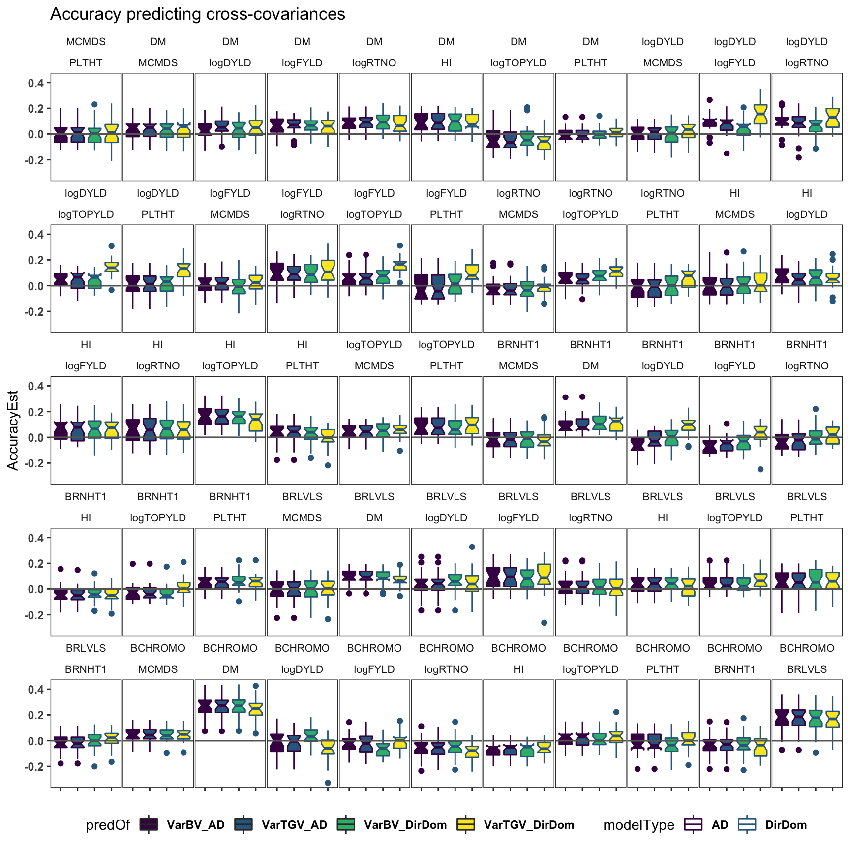
[TO REDO] Accuracy based only on large families
What if we only compute accuracy with families having >10 or >20 members?
# library(tidyverse); library(magrittr)
# cvvars<-readRDS(here::here("output","cvVarPredAccuracyAD.rds"))
#
# big_acc<-cvvars %>%
#   mutate(AccuracyEst_n10=map_dbl(predVSobs,function(predVSobs){
#     z<-predVSobs %>% filter(famSize>=10)
#     out<-psych::cor.wt(z[,c("predVar","obsVar")],
#                        w = z$famSize) %$% r[1,2] %>%
#       round(.,3)
#     return(out) }),
#     AccuracyEst_n20=map_dbl(predVSobs,function(predVSobs){
#       z<-predVSobs %>% filter(famSize>=20)
#       out<-psych::cor.wt(z[,c("predVar","obsVar")],
#                          w = z$famSize) %$% r[1,2] %>%
#         round(.,3)
#       return(out) }))
#
# big_acc %<>%
#   mutate(Trait1=factor(Trait1,levels=c("SELIND",blups$Trait)),
#          Trait2=factor(Trait2,levels=c("SELIND",blups$Trait)),
#          predOf=factor(predOf,levels=c("VarBV","VarTGV")))
#
# big_acc %>%
#   filter(Trait1==Trait2,predOf=="VarBV") %>%
#   select(-predVSobs) %>%
#   pivot_longer(cols = contains("Accuracy"), names_to = "FamilySizeForValidation",values_to = "AccuracyEst") %>%
#   ggplot(.,aes(x=predOf,y=AccuracyEst,fill=FamilySizeForValidation, color=predOf)) +
#   geom_boxplot(width=0.4,notch = TRUE,color='gray40') +
#   scale_fill_manual(values = viridis::viridis(4)[1:3]) +
#   #scale_color_manual(values = viridis::viridis(4)[1:3]) +
#   geom_hline(yintercept = 0, color='black', size=0.8) +
#   facet_grid(predOf~Trait1) +
#   labs(title="Accuracy predicting cross-variances in bigger famiilies only?") +
#   theme_bw() +
#   theme(axis.text.x = element_blank(),
#         axis.title.x = element_blank(),
#         strip.background = element_blank(),
#         panel.grid.major = element_blank(),
#         panel.grid.minor = element_blank(),
#         axis.text.y = element_text(face='bold'),
#         strip.text.x = element_text(face='bold'),
#         legend.position='bottom',
#         legend.text = element_text(face='bold'),
#         panel.spacing = unit(0.05, "lines"))
[RUNNING] Genomic Mate Selection
Placeholder for summaries of the full-model predictions of cross means and variances to-be-used for selection.
Genetic Gain Estimates
# GBLUPs
### Two models AD and DirDom
#gpreds_ad<-readRDS(file = here::here("output","genomicPredictions_ModelAD.rds"))
gpreds_dirdom<-readRDS(file = here::here("output","genomicPredictions_ModelDirDom.rds"))
si_getgvs<-gpreds_dirdom$gblups[[1]] %>%
#si_getgvs<-gpreds_ad$gblups[[1]] %>%
  filter(predOf=="GETGV") %>%
  select(GID,SELIND)

## IITA Germplasm Ages
ggcycletime<-readxl::read_xls(here::here("data","PedigreeGeneticGainCycleTime_aafolabi_01122020.xls")) %>%
  mutate(Year_Accession=as.numeric(Year_Accession))

# Need germplasmName field from raw trial data to match GEBV and cycle time
rawdata<-readRDS(here::here("output","IITA_ExptDesignsDetected_2021May10.rds"))
si_getgvs %<>%
  left_join(rawdata %>%
              distinct(germplasmName,GID)) %>%
  group_by(GID) %>%
  slice(1) %>%
  ungroup()
# table(ggcycletime$Accession %in% si_getgvs$germplasmName)
# FALSE  TRUE
#   193   614

si_getgvs %<>%
  left_join(.,ggcycletime %>%
              rename(germplasmName=Accession) %>%
              mutate(Year_Accession=as.numeric(Year_Accession))) %>%
  mutate(Year_Accession=case_when(grepl("2013_|TMS13",germplasmName)~2013,
                                  grepl("TMS14",germplasmName)~2014,
                                  grepl("TMS15",germplasmName)~2015,
                                  grepl("TMS18",germplasmName)~2018,
                                  !grepl("2013_|TMS13|TMS14|TMS15|TMS18",germplasmName)~Year_Accession))

# Declare the "eras" as PreGS\<2012 and GS\>=2013.
si_getgvs %<>%
  filter(Year_Accession>2012 | Year_Accession<2005)
si_getgvs %<>%
  mutate(GeneticGroup=ifelse(Year_Accession>=2013,"GS","PreGS"))
Show rate of genetic gain - getgv vs. accession age
# , fig.height=10, fig.width=12
si_getgvs %>%
select(GeneticGroup,GID,Year_Accession,SELIND) %>%
ggplot(.,aes(x=Year_Accession,y=SELIND,color=GeneticGroup)) +
geom_point(size=1.25) + geom_smooth(method=lm, se=TRUE, size=1.5) +
# facet_wrap(~Trait,scales='free_y', ncol=2) +
theme_bw() +
theme(axis.text = element_text(face = 'bold',angle = 0, size=14),
axis.title = element_text(face = 'bold',size=16),
strip.background.x = element_blank(),
strip.text = element_text(face='bold',size=18)) +
scale_color_viridis_d() +
labs(title = "Selection Index GETGV vs. Accession Age by 'era' [GS vs. PreGS]",
subtitle = "SI GETGV from modelType='DirDom'")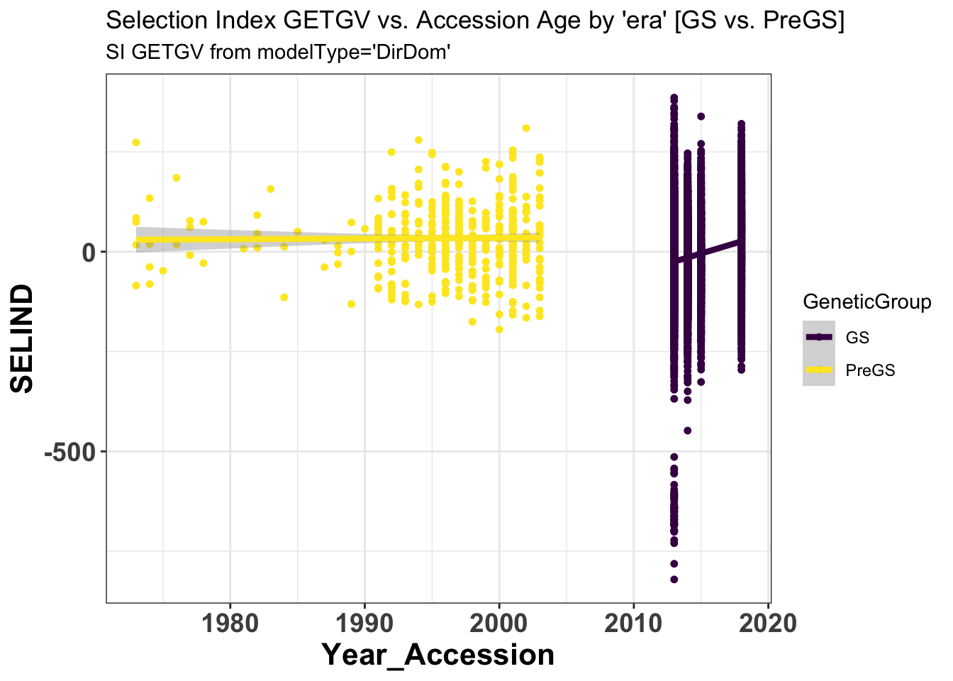 Barplot of mean GEBV vs. Cycle
si_gebvs<-gpreds_dirdom$gblups[[1]] %>%
  filter(predOf=="GEBV") %>%
  select(GID,SELIND) %>%
  mutate(GeneticGroup=case_when(grepl("2013_|TMS13",GID)~"C1",
                                  grepl("TMS14",GID)~"C2",
                                  grepl("TMS15",GID)~"C3",
                                  grepl("TMS18",GID)~"C4",
                                  !grepl("2013_|TMS13|TMS14|TMS15|TMS18",GID)~"PreGS"),
         GeneticGroup=factor(GeneticGroup,levels = c("PreGS","C1","C2","C3","C4")))
si_gebvs %>%
  group_by(GeneticGroup) %>%
  summarize(meanGEBV=mean(SELIND),
            stdErr=sd(SELIND)/sqrt(n()),
            upperSE=meanGEBV+stdErr,
            lowerSE=meanGEBV-stdErr) %>%
  ggplot(.,aes(x=GeneticGroup,y=meanGEBV,fill=GeneticGroup)) +
  geom_bar(stat = 'identity', color='gray60', size=1.25) +
  geom_linerange(aes(ymax=upperSE,
                     ymin=lowerSE), color='gray60', size=1.25) +
  #facet_wrap(~Trait,scales='free_y', ncol=1) +
  theme_bw() +
  geom_hline(yintercept = 0, size=1.15, color='black') +
  theme(axis.text.x = element_text(face = 'bold',angle = 0, size=12),
        axis.title.y = element_text(face = 'bold',size=14),
        legend.position = 'none',
        strip.background.x = element_blank(),
        strip.text = element_text(face='bold',size=14)) +
  scale_fill_viridis_d() +
  labs(x=NULL,y="Mean GEBVs",
       title="Mean +/- Std. Error Selection Index GEBV by Cycle")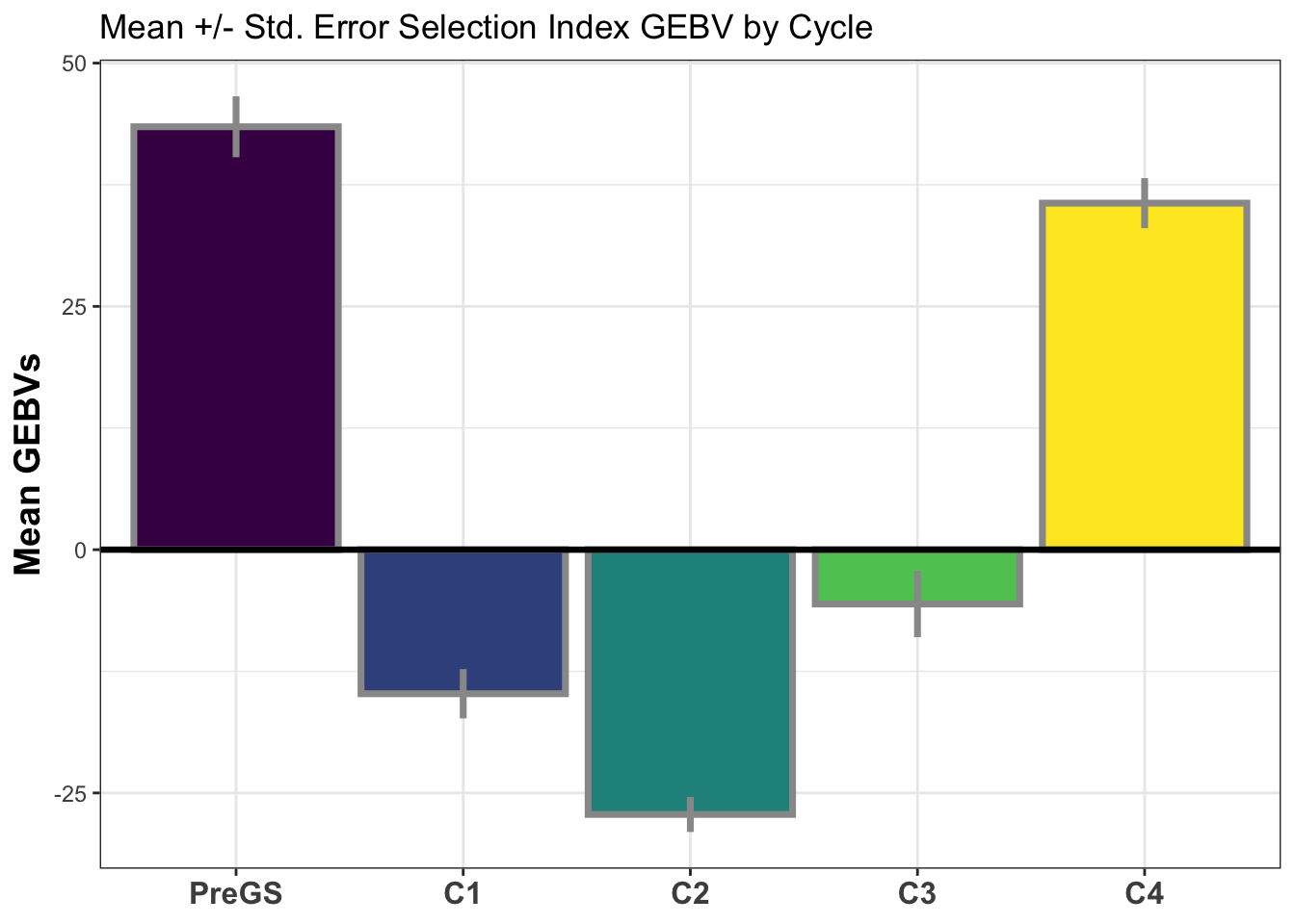
sessionInfo()R version 4.1.0 (2021-05-18)
Platform: x86_64-apple-darwin17.0 (64-bit)
Running under: macOS Big Sur 10.16
Matrix products: default
BLAS: /Library/Frameworks/R.framework/Versions/4.1/Resources/lib/libRblas.dylib
LAPACK: /Library/Frameworks/R.framework/Versions/4.1/Resources/lib/libRlapack.dylib
locale:
[1] en_US.UTF-8/en_US.UTF-8/en_US.UTF-8/C/en_US.UTF-8/en_US.UTF-8
attached base packages:
[1] stats graphics grDevices utils datasets methods base
other attached packages:
[1] ggdist_2.4.1 ragg_1.1.3 magrittr_2.0.1 forcats_0.5.1
[5] stringr_1.4.0 dplyr_1.0.7 purrr_0.3.4 readr_1.4.0
[9] tidyr_1.1.3 tibble_3.1.2 ggplot2_3.3.5 tidyverse_1.3.1
[13] workflowr_1.6.2
loaded via a namespace (and not attached):
[1] viridis_0.6.1 httr_1.4.2 sass_0.4.0
[4] jsonlite_1.7.2 viridisLite_0.4.0 splines_4.1.0
[7] here_1.0.1 modelr_0.1.8 bslib_0.2.5.1
[10] assertthat_0.2.1 distributional_0.2.2 highr_0.9
[13] cellranger_1.1.0 yaml_2.2.1 lattice_0.20-44
[16] pillar_1.6.1 backports_1.2.1 glue_1.4.2
[19] digest_0.6.27 promises_1.2.0.1 rvest_1.0.0
[22] colorspace_2.0-2 Matrix_1.3-4 htmltools_0.5.1.1
[25] httpuv_1.6.1 pkgconfig_2.0.3 broom_0.7.8
[28] haven_2.4.1 scales_1.1.1 whisker_0.4
[31] later_1.2.0 git2r_0.28.0 mgcv_1.8-36
[34] generics_0.1.0 farver_2.1.0 ellipsis_0.3.2
[37] withr_2.4.2 cli_3.0.0 crayon_1.4.1
[40] readxl_1.3.1 evaluate_0.14 fs_1.5.0
[43] fansi_0.5.0 nlme_3.1-152 xml2_1.3.2
[46] beeswarm_0.4.0 textshaping_0.3.5 tools_4.1.0
[49] hms_1.1.0 lifecycle_1.0.0 munsell_0.5.0
[52] reprex_2.0.0 compiler_4.1.0 jquerylib_0.1.4
[55] systemfonts_1.0.2 rlang_0.4.11 grid_4.1.0
[58] rstudioapi_0.13 labeling_0.4.2 rmarkdown_2.9
[61] gtable_0.3.0 DBI_1.1.1 R6_2.5.0
[64] gridExtra_2.3 lubridate_1.7.10 knitr_1.33
[67] utf8_1.2.1 rprojroot_2.0.2 stringi_1.6.2
[70] Rcpp_1.0.7 vctrs_0.3.8 dbplyr_2.1.1
[73] tidyselect_1.1.1 xfun_0.24