model_fitting

workflowr

• Summary
• Checks
• Past versions

Last updated: 2020-07-22

Checks: 6 1

Knit directory: gene_level_fine_mapping/

This reproducible R Markdown analysis was created with workflowr (version 1.6.1). The Checks tab describes the reproducibility checks that were applied when the results were created. The Past versions tab lists the development history.

---

R Markdown file: up-to-date

Great! Since the R Markdown file has been committed to the Git repository, you know the exact version of the code that produced these results.

Environment: empty

Great job! The global environment was empty. Objects defined in the global environment can affect the analysis in your R Markdown file in unknown ways. For reproduciblity it’s best to always run the code in an empty environment.

Seed: set.seed(20200622)

The command set.seed(20200622) was run prior to running the code in the R Markdown file. Setting a seed ensures that any results that rely on randomness, e.g. subsampling or permutations, are reproducible.

Session information: recorded

Great job! Recording the operating system, R version, and package versions is critical for reproducibility.

Cache: none

Nice! There were no cached chunks for this analysis, so you can be confident that you successfully produced the results during this run.

File paths: absolute

Using absolute paths to the files within your workflowr project makes it difficult for you and others to run your code on a different machine. Change the absolute path(s) below to the suggested relative path(s) to make your code more reproducible.

absolute	relative
/Users/nicholeyang/Desktop/gene_level_fine_mapping/data/training.RData	data/training.RData

Repository version: 8e990ec

Great! You are using Git for version control. Tracking code development and connecting the code version to the results is critical for reproducibility.

The results in this page were generated with repository version 8e990ec. See the Past versions tab to see a history of the changes made to the R Markdown and HTML files.

Note that you need to be careful to ensure that all relevant files for the analysis have been committed to Git prior to generating the results (you can use wflow_publish or wflow_git_commit). workflowr only checks the R Markdown file, but you know if there are other scripts or data files that it depends on. Below is the status of the Git repository when the results were generated:

Ignored files:
    Ignored:    .DS_Store
    Ignored:    .Rhistory
    Ignored:    .Rproj.user/

Note that any generated files, e.g. HTML, png, CSS, etc., are not included in this status report because it is ok for generated content to have uncommitted changes.

---

These are the previous versions of the repository in which changes were made to the R Markdown (analysis/model_fitting.Rmd) and HTML (docs/model_fitting.html) files. If you’ve configured a remote Git repository (see ?wflow_git_remote), click on the hyperlinks in the table below to view the files as they were in that past version.

File	Version	Author	Date	Message
Rmd	8e990ec	yunqiyang0215	2020-07-22	wflow_publish(“analysis/model_fitting.Rmd”)
html	da6a45b	yunqiyang0215	2020-07-21	Build site.
Rmd	98a26e9	yunqiyang0215	2020-07-21	wflow_publish(“analysis/model_fitting.Rmd”)

---

library(ggplot2)
library(dplyr)

Attaching package: 'dplyr'

The following objects are masked from 'package:stats':

    filter, lag

The following objects are masked from 'package:base':

    intersect, setdiff, setequal, union

require(PRROC)

Loading required package: PRROC

load("/Users/nicholeyang/Desktop/gene_level_fine_mapping/data/training.RData")

## remove NAs
dat = rbind(train_pos_all, train_neg_all)
NAs = apply(dat, 1, function(x) sum(is.na(x)))
dat = dat[NAs == 0, ]

data overview

head(dat)

  gene_name             variant_id UTR5 UTR3 exon intron upstream
1    LRRC39 chr1_100178174_A_G_b38    1    0    0      0        0
2     EXTL2 chr1_100895622_C_T_b38    0    0    0      0        1
3     KIF1B  chr1_10211630_C_G_b38    1    0    0      0        0
6  SLC25A24 chr1_108199501_C_G_b38    0    0    0      1        0
8     TAF13 chr1_109076695_G_A_b38    0    0    0      0        1
9  C1orf194 chr1_109113015_C_A_b38    0    0    0      1        0
  tss_dist_to_snp y
1              41 1
2             376 1
3              14 1
6             857 1
8             693 1
9             268 1

# number of observations in the dataset 
dim(dat)[1]

[1] 65858

sum(dat$y == 1)  # positive pairs

[1] 3828

sum(dat$y == 0)  # negative pairs 

[1] 62030

proportion of features

par(mfrow = c(1,2))

# proportion of features in the positive set
tot_count = apply(dat[dat$y==1, c(3:7)], 2, function(x) sum(x == 1))
barplot(tot_count/dim(dat[dat$y==1, ])[1], las = 2, main = 'feature proportion in positive set')

# proportion of features in the negative set
tot_count = apply(dat[dat$y==0, c(3:7)], 2, function(x) sum(x == 1))
barplot(tot_count/dim(dat[dat$y==0, ])[1], ylim = c(0, 0.01), las = 2, main = 'feature proportion in negative set')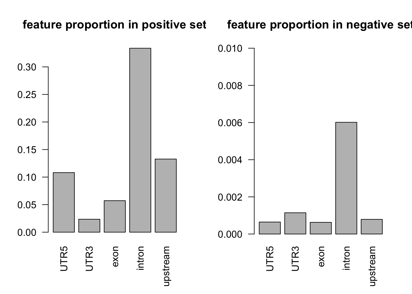

by variable logistic regression

fit1  = glm(y ~ UTR5, data = dat, family = "binomial")
fit2 = glm(y ~ UTR3, data = dat, family = "binomial")
fit3 = glm(y ~ exon, data = dat, family = "binomial")
fit4 = glm(y ~ intron, data = dat, family = "binomial")
fit5 = glm(y ~ upstream, data = dat, family = "binomial")


summary(fit1)

Call:
glm(formula = y ~ UTR5, family = "binomial", data = dat)

Deviance Residuals: 
    Min       1Q   Median       3Q      Max  
-2.2042  -0.3275  -0.3275  -0.3275   2.4301  

Coefficients:
            Estimate Std. Error z value Pr(>|z|)    
(Intercept) -2.89909    0.01758 -164.92   <2e-16 ***
UTR5         5.23607    0.16651   31.45   <2e-16 ***
---
Signif. codes:  0 '***' 0.001 '**' 0.01 '*' 0.05 '.' 0.1 ' ' 1

(Dispersion parameter for binomial family taken to be 1)

    Null deviance: 29212  on 65857  degrees of freedom
Residual deviance: 27078  on 65856  degrees of freedom
AIC: 27082

Number of Fisher Scoring iterations: 5

summary(fit2)

Call:
glm(formula = y ~ UTR3, family = "binomial", data = dat)

Deviance Residuals: 
    Min       1Q   Median       3Q      Max  
-1.2796  -0.3423  -0.3423  -0.3423   2.3944  

Coefficients:
            Estimate Std. Error z value Pr(>|z|)    
(Intercept) -2.80792    0.01684 -166.72   <2e-16 ***
UTR3         3.04505    0.15962   19.08   <2e-16 ***
---
Signif. codes:  0 '***' 0.001 '**' 0.01 '*' 0.05 '.' 0.1 ' ' 1

(Dispersion parameter for binomial family taken to be 1)

    Null deviance: 29212  on 65857  degrees of freedom
Residual deviance: 28910  on 65856  degrees of freedom
AIC: 28914

Number of Fisher Scoring iterations: 5

summary(fit3)

Call:
glm(formula = y ~ exon, family = "binomial", data = dat)

Deviance Residuals: 
    Min       1Q   Median       3Q      Max  
-1.9439  -0.3364  -0.3364  -0.3364   2.4084  

Coefficients:
            Estimate Std. Error z value Pr(>|z|)    
(Intercept) -2.84356    0.01712 -166.06   <2e-16 ***
exon         4.56907    0.17464   26.16   <2e-16 ***
---
Signif. codes:  0 '***' 0.001 '**' 0.01 '*' 0.05 '.' 0.1 ' ' 1

(Dispersion parameter for binomial family taken to be 1)

    Null deviance: 29212  on 65857  degrees of freedom
Residual deviance: 28168  on 65856  degrees of freedom
AIC: 28172

Number of Fisher Scoring iterations: 5

summary(fit4)

Call:
glm(formula = y ~ intron, family = "binomial", data = dat)

Deviance Residuals: 
    Min       1Q   Median       3Q      Max  
-1.7248  -0.2847  -0.2847  -0.2847   2.5401  

Coefficients:
            Estimate Std. Error z value Pr(>|z|)    
(Intercept) -3.18549    0.02021 -157.63   <2e-16 ***
intron       4.41697    0.06222   70.98   <2e-16 ***
---
Signif. codes:  0 '***' 0.001 '**' 0.01 '*' 0.05 '.' 0.1 ' ' 1

(Dispersion parameter for binomial family taken to be 1)

    Null deviance: 29212  on 65857  degrees of freedom
Residual deviance: 23214  on 65856  degrees of freedom
AIC: 23218

Number of Fisher Scoring iterations: 6

summary(fit5)

Call:
glm(formula = y ~ upstream, family = "binomial", data = dat)

Deviance Residuals: 
    Min       1Q   Median       3Q      Max  
-2.2049  -0.3231  -0.3231  -0.3231   2.4409  

Coefficients:
            Estimate Std. Error z value Pr(>|z|)    
(Intercept) -2.92686    0.01781 -164.31   <2e-16 ***
upstream     5.26552    0.15065   34.95   <2e-16 ***
---
Signif. codes:  0 '***' 0.001 '**' 0.01 '*' 0.05 '.' 0.1 ' ' 1

(Dispersion parameter for binomial family taken to be 1)

    Null deviance: 29212  on 65857  degrees of freedom
Residual deviance: 26581  on 65856  degrees of freedom
AIC: 26585

Number of Fisher Scoring iterations: 5

fit all features

fit6 = glm(y ~ UTR5 + intron + upstream + exon, data = dat, family = "binomial")
summary(fit6)

Call:
glm(formula = y ~ UTR5 + intron + upstream + exon, family = "binomial", 
    data = dat)

Deviance Residuals: 
    Min       1Q   Median       3Q      Max  
-2.2049  -0.2128  -0.2128  -0.2128   2.7565  

Coefficients:
            Estimate Std. Error z value Pr(>|z|)    
(Intercept) -3.77663    0.02694 -140.17   <2e-16 ***
UTR5         6.11361    0.16775   36.44   <2e-16 ***
intron       5.00810    0.06473   77.38   <2e-16 ***
upstream     6.11529    0.15200   40.23   <2e-16 ***
exon         5.50214    0.17588   31.28   <2e-16 ***
---
Signif. codes:  0 '***' 0.001 '**' 0.01 '*' 0.05 '.' 0.1 ' ' 1

(Dispersion parameter for binomial family taken to be 1)

    Null deviance: 29212  on 65857  degrees of freedom
Residual deviance: 16078  on 65853  degrees of freedom
AIC: 16088

Number of Fisher Scoring iterations: 6

fit7 = glm(y ~ UTR5 + UTR3 + intron + upstream + exon, data = dat, family = "binomial")
summary(fit7)

Call:
glm(formula = y ~ UTR5 + UTR3 + intron + upstream + exon, family = "binomial", 
    data = dat)

Deviance Residuals: 
    Min       1Q   Median       3Q      Max  
-2.2049  -0.2061  -0.2061  -0.2061   2.7795  

Coefficients:
            Estimate Std. Error z value Pr(>|z|)    
(Intercept) -3.84148    0.02783 -138.05   <2e-16 ***
UTR5         6.17847    0.16790   36.80   <2e-16 ***
UTR3         4.07861    0.16115   25.31   <2e-16 ***
intron       5.07295    0.06510   77.93   <2e-16 ***
upstream     6.18014    0.15215   40.62   <2e-16 ***
exon         5.56699    0.17602   31.63   <2e-16 ***
---
Signif. codes:  0 '***' 0.001 '**' 0.01 '*' 0.05 '.' 0.1 ' ' 1

(Dispersion parameter for binomial family taken to be 1)

    Null deviance: 29212  on 65857  degrees of freedom
Residual deviance: 15607  on 65852  degrees of freedom
AIC: 15619

Number of Fisher Scoring iterations: 6

AIC criteria and deviance: the smaller the better

\[AIC=-2\log L(\theta)+2k\] \[deviance=-2\log L(\theta)\]

calculate prediction accuracy: train-test split

set.seed(1)
n = dim(dat)[1]
indx = sample(1:n, round(2*n/3), replace = FALSE)
train = dat[indx, ]
test = dat[-indx, ]

# build model on the training set
fit.all = glm(y ~ UTR5 + UTR3 + intron + upstream + exon, data = train, family = "binomial")

# evaluate on the test set 
pred.probs=predict(fit.all,test,type="response")

plot(pred.probs, type = 'p', pch = '.')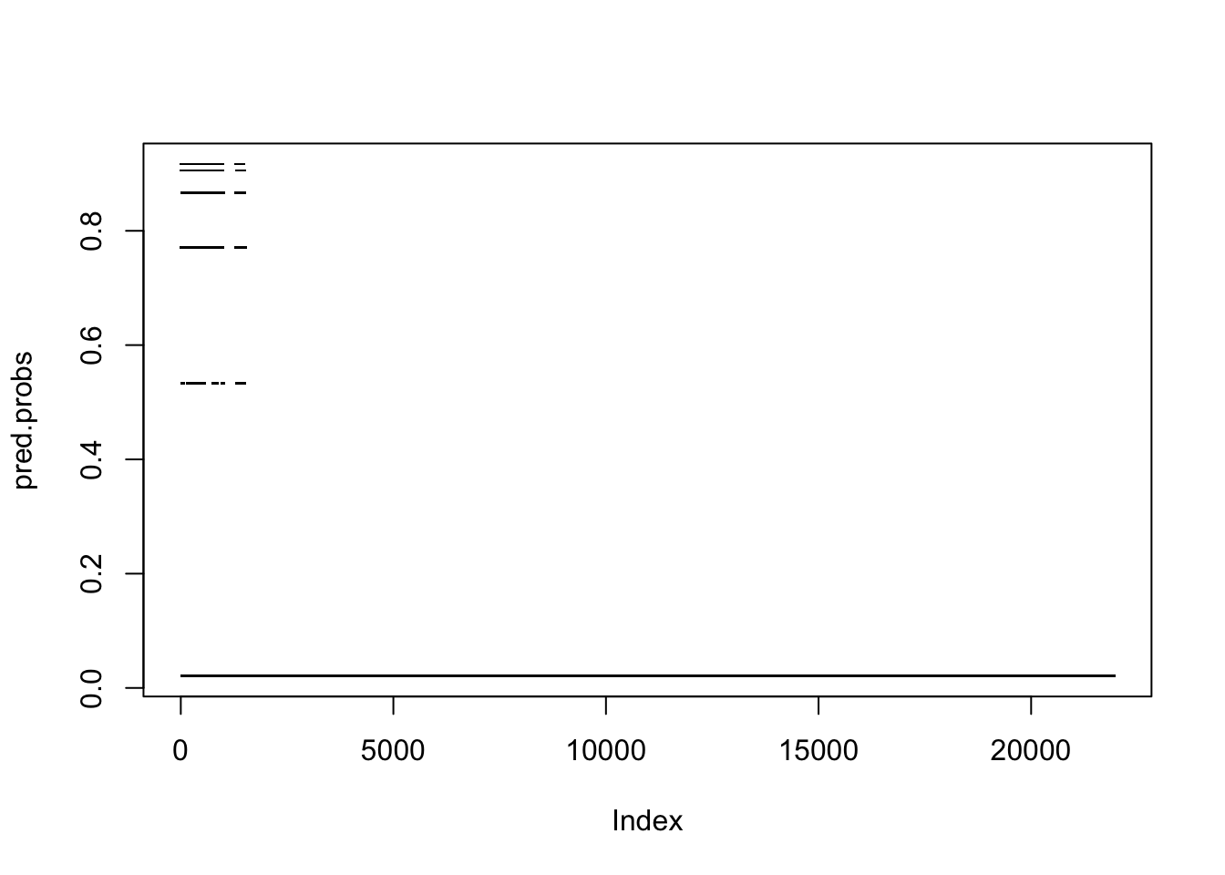

classification accuracy

glm.pred = rep(0, length(pred.probs))
glm.pred[pred.probs>0.5]= 1
table(glm.pred, test$y)

        
glm.pred     0     1
       0 20496   446
       1   184   827

plot ROC-AUC PR-AUC

fg <- pred.probs[test$y == 1]
bg <- pred.probs[test$y== 0]

# ROC Curve    
roc <- roc.curve(scores.class0 = fg, scores.class1 = bg, curve = T)
plot(roc)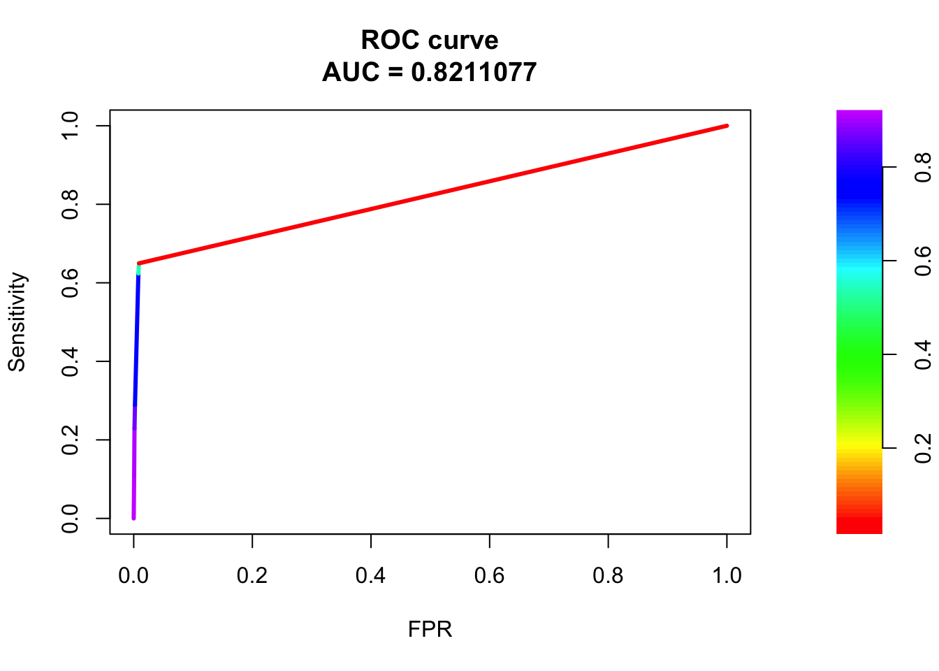

# PR Curve
pr <- pr.curve(scores.class0 = fg, scores.class1 = bg, curve = T)
plot(pr)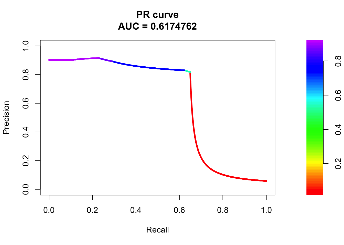

play around tss feature

summary(dat$tss_dist_to_snp)

   Min. 1st Qu.  Median    Mean 3rd Qu.    Max. 
      0   91718  221543  232448  364130 2176373 

summary(dat[dat$y==1, ]$tss_dist_to_snp)  # dist_to_tss in positive set 

    Min.  1st Qu.   Median     Mean  3rd Qu.     Max. 
     0.0    297.8   3009.5  20349.3  17583.0 946399.0 

summary(dat[dat$y==0, ]$tss_dist_to_snp)  # dist_to_tss in negative set 

   Min. 1st Qu.  Median    Mean 3rd Qu.    Max. 
      0  112052  237240  245537  372089 2176373 

# change fill and outline color manually 
ggplot(dat, aes(x = tss_dist_to_snp)) +
  geom_histogram(aes(color = as.factor(y), fill = as.factor(y)), 
                position = "identity", bins = 50, alpha = 0.4) +
  scale_color_manual(values = c("#00AFBB", "#E7B800")) +
  scale_fill_manual(values = c("#00AFBB", "#E7B800"))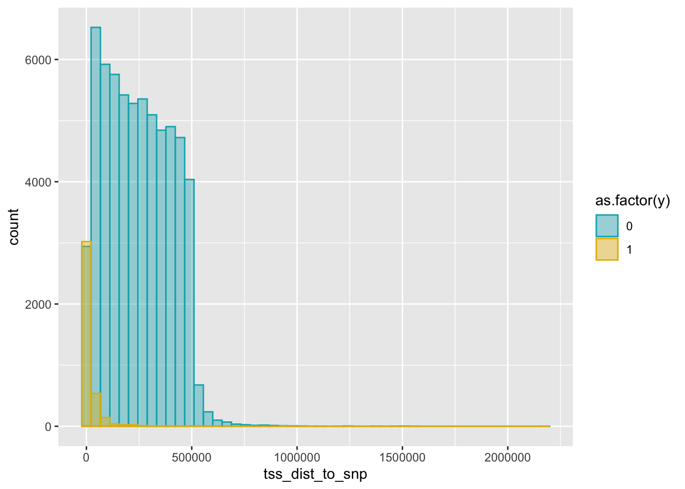

boxplot(tss_dist_to_snp ~ y, data = dat)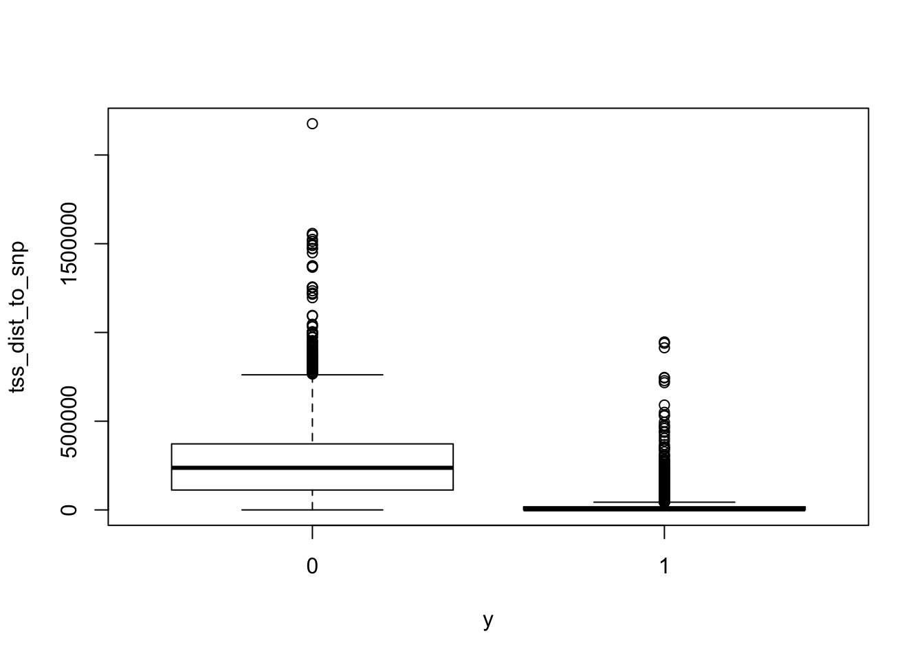

exponential decay: exp(-d/sigma)

sigma = 1e5
dat$weight = exp(-dat$tss_dist_to_snp/sigma)

# change fill and outline color manually 
ggplot(dat, aes(x = weight)) +
  geom_histogram(aes(color = as.factor(y), fill = as.factor(y)), 
                position = "identity", bins = 50, alpha = 0.4) +
  scale_color_manual(values = c("#00AFBB", "#E7B800")) +
  scale_fill_manual(values = c("#00AFBB", "#E7B800"))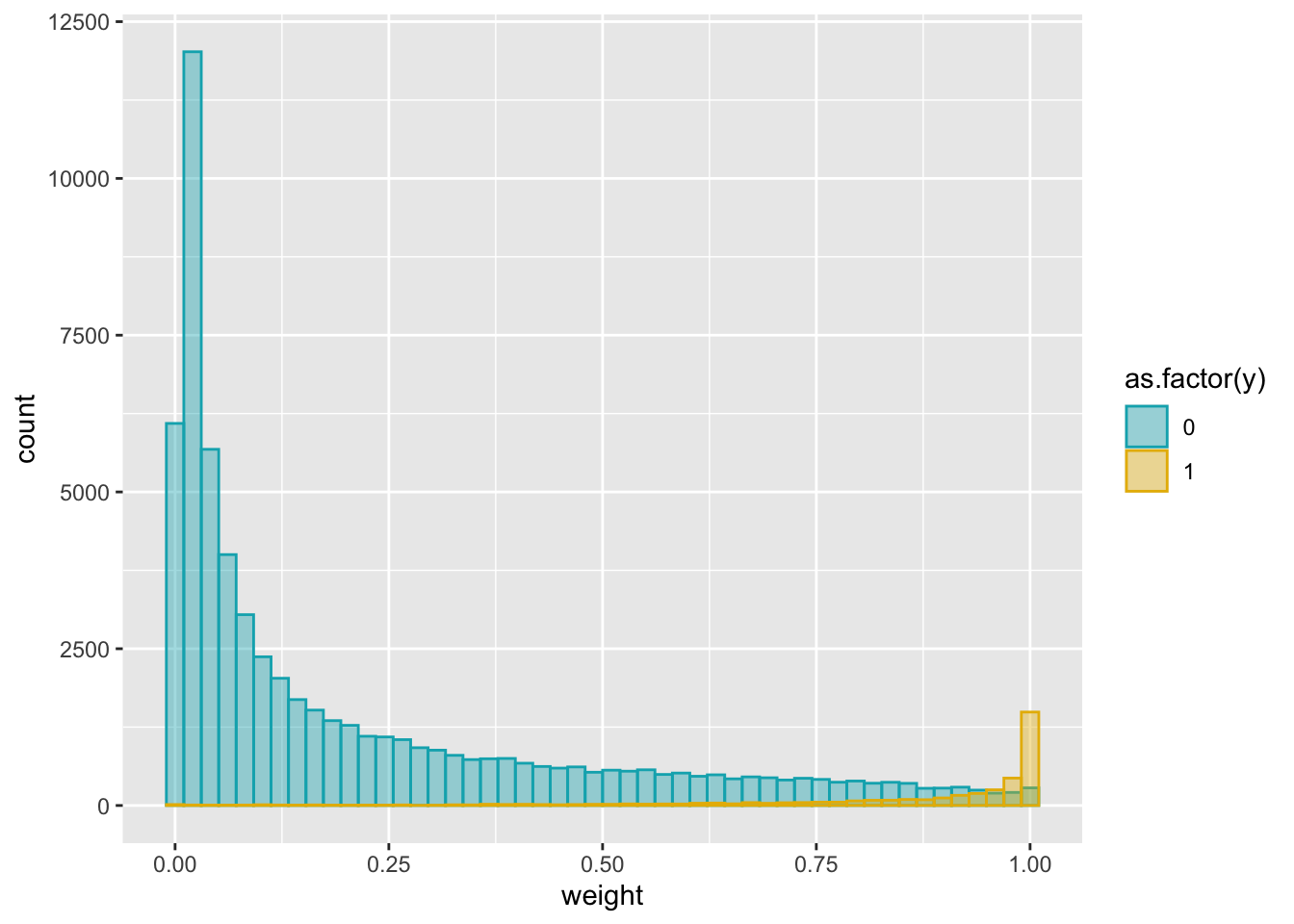

boxplot(weight ~ y, data = dat)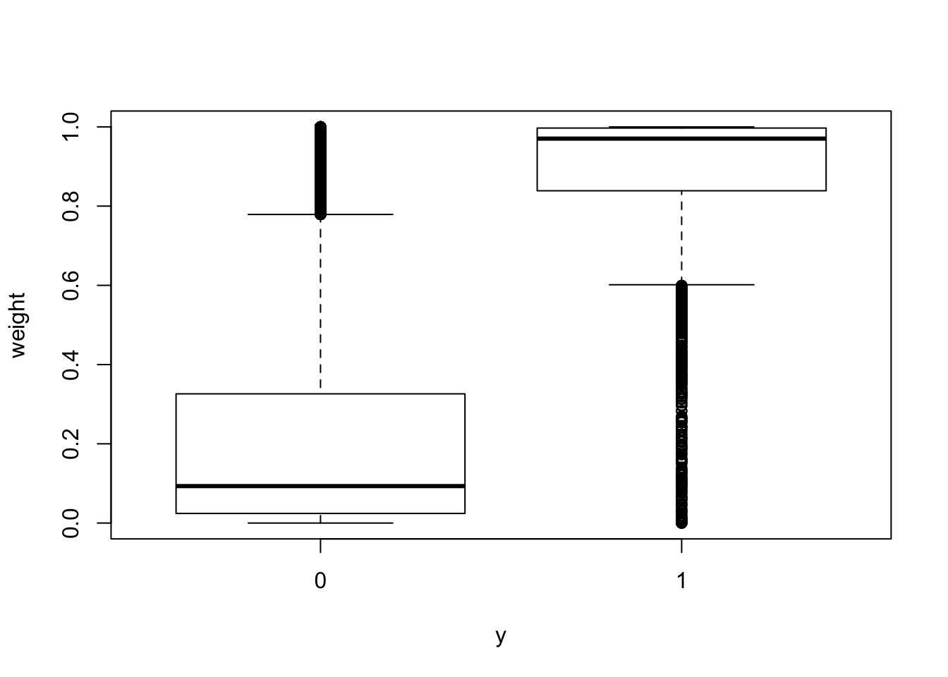

# fit raw tss
fit.raw.tss  = glm(y ~ tss_dist_to_snp, data = dat, family = "binomial")

Warning: glm.fit: fitted probabilities numerically 0 or 1 occurred

summary(fit.raw.tss)

Call:
glm(formula = y ~ tss_dist_to_snp, family = "binomial", data = dat)

Deviance Residuals: 
    Min       1Q   Median       3Q      Max  
-1.1726  -0.1247  -0.0083  -0.0004   8.4904  

Coefficients:
                  Estimate Std. Error z value Pr(>|z|)    
(Intercept)     -1.134e-02  2.724e-02  -0.416    0.677    
tss_dist_to_snp -4.057e-05  7.292e-07 -55.626   <2e-16 ***
---
Signif. codes:  0 '***' 0.001 '**' 0.01 '*' 0.05 '.' 0.1 ' ' 1

(Dispersion parameter for binomial family taken to be 1)

    Null deviance: 29212  on 65857  degrees of freedom
Residual deviance: 15906  on 65856  degrees of freedom
AIC: 15910

Number of Fisher Scoring iterations: 10

# fit exponential decay: 
fit.exp.tss  = glm(y ~ weight, data = dat, family = "binomial")
summary(fit.exp.tss)

Call:
glm(formula = y ~ weight, family = "binomial", data = dat)

Deviance Residuals: 
    Min       1Q   Median       3Q      Max  
-1.4245  -0.1030  -0.0406  -0.0315   3.9398  

Coefficients:
            Estimate Std. Error z value Pr(>|z|)    
(Intercept) -7.76129    0.09819  -79.05   <2e-16 ***
weight       8.32556    0.11643   71.50   <2e-16 ***
---
Signif. codes:  0 '***' 0.001 '**' 0.01 '*' 0.05 '.' 0.1 ' ' 1

(Dispersion parameter for binomial family taken to be 1)

    Null deviance: 29212  on 65857  degrees of freedom
Residual deviance: 14000  on 65856  degrees of freedom
AIC: 14004

Number of Fisher Scoring iterations: 8

add weight to all feature logsitic regression and plot ROC/PR-AUC

# split data in the same way
set.seed(1)
n = dim(dat)[1]
indx = sample(1:n, round(2*n/3), replace = FALSE)
train = dat[indx, ]
test = dat[-indx, ]

# fit model and evaluate performance
fit.all = glm(y ~ UTR5 + UTR3 + intron + upstream + exon + weight, data = train, family = "binomial")
summary(fit.all)

Call:
glm(formula = y ~ UTR5 + UTR3 + intron + upstream + exon + weight, 
    family = "binomial", data = train)

Deviance Residuals: 
    Min       1Q   Median       3Q      Max  
-2.3112  -0.1202  -0.0614  -0.0513   3.6728  

Coefficients:
            Estimate Std. Error z value Pr(>|z|)    
(Intercept) -6.74427    0.10647 -63.343  < 2e-16 ***
UTR5         3.29539    0.22171  14.863  < 2e-16 ***
UTR3         1.73510    0.21358   8.124 4.51e-16 ***
intron       2.99398    0.09153  32.710  < 2e-16 ***
upstream     3.38742    0.19178  17.663  < 2e-16 ***
exon         3.42179    0.26956  12.694  < 2e-16 ***
weight       5.97896    0.13754  43.471  < 2e-16 ***
---
Signif. codes:  0 '***' 0.001 '**' 0.01 '*' 0.05 '.' 0.1 ' ' 1

(Dispersion parameter for binomial family taken to be 1)

    Null deviance: 19491.1  on 43904  degrees of freedom
Residual deviance:  7377.4  on 43898  degrees of freedom
AIC: 7391.4

Number of Fisher Scoring iterations: 8

pred.probs=predict(fit.all,test,type="response")
glm.pred = rep(0, length(pred.probs))
glm.pred[pred.probs>0.5]= 1
table(glm.pred, test$y)

        
glm.pred     0     1
       0 20539   503
       1   141   770

fg <- pred.probs[test$y == 1]
bg <- pred.probs[test$y== 0]

# ROC Curve    
roc <- roc.curve(scores.class0 = fg, scores.class1 = bg, curve = T)
plot(roc)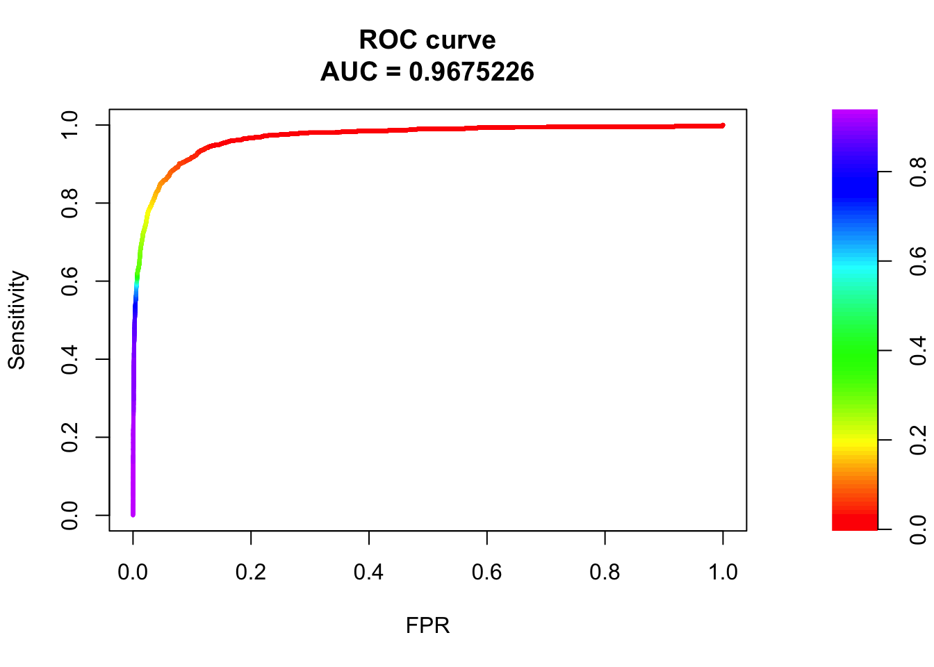

# PR Curve
pr <- pr.curve(scores.class0 = fg, scores.class1 = bg, curve = T)
plot(pr)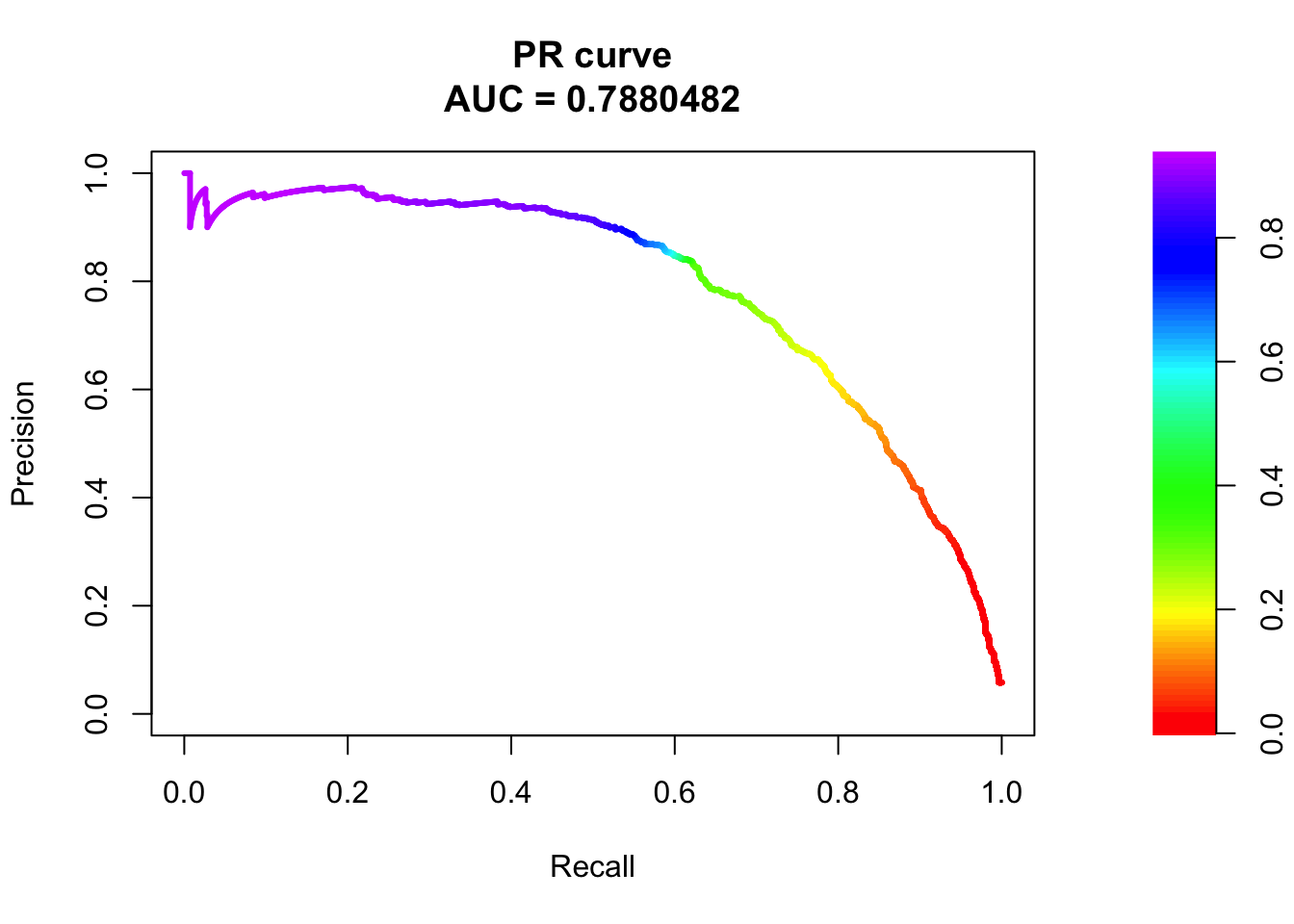

Session information

sessionInfo()

R version 3.6.3 (2020-02-29)
Platform: x86_64-apple-darwin15.6.0 (64-bit)
Running under: macOS Catalina 10.15.5

Matrix products: default
BLAS:   /Library/Frameworks/R.framework/Versions/3.6/Resources/lib/libRblas.0.dylib
LAPACK: /Library/Frameworks/R.framework/Versions/3.6/Resources/lib/libRlapack.dylib

locale:
[1] en_US.UTF-8/en_US.UTF-8/en_US.UTF-8/C/en_US.UTF-8/en_US.UTF-8

attached base packages:
[1] stats     graphics  grDevices utils     datasets  methods   base     

other attached packages:
[1] PRROC_1.3.1     dplyr_0.8.5     ggplot2_3.3.0   workflowr_1.6.1

loaded via a namespace (and not attached):
 [1] Rcpp_1.0.4       compiler_3.6.3   pillar_1.4.3     later_1.0.0     
 [5] git2r_0.26.1     highr_0.8        tools_3.6.3      digest_0.6.25   
 [9] evaluate_0.14    lifecycle_0.2.0  tibble_3.0.1     gtable_0.3.0    
[13] pkgconfig_2.0.3  rlang_0.4.5      rstudioapi_0.11  yaml_2.2.1      
[17] xfun_0.12        withr_2.1.2      stringr_1.4.0    knitr_1.28      
[21] fs_1.3.2         vctrs_0.2.4      rprojroot_1.3-2  grid_3.6.3      
[25] tidyselect_1.0.0 glue_1.3.2       R6_2.4.1         rmarkdown_2.1   
[29] farver_2.0.3     purrr_0.3.3      magrittr_1.5     whisker_0.4     
[33] backports_1.1.5  scales_1.1.0     promises_1.1.0   htmltools_0.4.0 
[37] ellipsis_0.3.0   assertthat_0.2.1 colorspace_1.4-1 httpuv_1.5.2    
[41] labeling_0.3     stringi_1.4.6    munsell_0.5.0    crayon_1.3.4