sim_survival

workflowr

• Summary
• Checks
• Past versions

Last updated: 2023-02-06

Checks: 7 0

Knit directory: survival-susie/

This reproducible R Markdown analysis was created with workflowr (version 1.6.2). The Checks tab describes the reproducibility checks that were applied when the results were created. The Past versions tab lists the development history.

---

R Markdown file: up-to-date

Great! Since the R Markdown file has been committed to the Git repository, you know the exact version of the code that produced these results.

Environment: empty

Great job! The global environment was empty. Objects defined in the global environment can affect the analysis in your R Markdown file in unknown ways. For reproduciblity it’s best to always run the code in an empty environment.

Seed: set.seed(20230201)

The command set.seed(20230201) was run prior to running the code in the R Markdown file. Setting a seed ensures that any results that rely on randomness, e.g. subsampling or permutations, are reproducible.

Session information: recorded

Great job! Recording the operating system, R version, and package versions is critical for reproducibility.

Cache: none

Nice! There were no cached chunks for this analysis, so you can be confident that you successfully produced the results during this run.

File paths: relative

Great job! Using relative paths to the files within your workflowr project makes it easier to run your code on other machines.

Repository version: bf1a95e

Great! You are using Git for version control. Tracking code development and connecting the code version to the results is critical for reproducibility.

The results in this page were generated with repository version bf1a95e. See the Past versions tab to see a history of the changes made to the R Markdown and HTML files.

Note that you need to be careful to ensure that all relevant files for the analysis have been committed to Git prior to generating the results (you can use wflow_publish or wflow_git_commit). workflowr only checks the R Markdown file, but you know if there are other scripts or data files that it depends on. Below is the status of the Git repository when the results were generated:

Ignored files:
    Ignored:    .DS_Store
    Ignored:    .Rhistory
    Ignored:    .Rproj.user/
    Ignored:    analysis/.RData
    Ignored:    analysis/.Rhistory

Untracked files:
    Untracked:  analysis/ser_survival.Rmd
    Untracked:  data/sim1.rds

Note that any generated files, e.g. HTML, png, CSS, etc., are not included in this status report because it is ok for generated content to have uncommitted changes.

---

These are the previous versions of the repository in which changes were made to the R Markdown (analysis/sim_survival.Rmd) and HTML (docs/sim_survival.html) files. If you’ve configured a remote Git repository (see ?wflow_git_remote), click on the hyperlinks in the table below to view the files as they were in that past version.

File	Version	Author	Date	Message
Rmd	bf1a95e	yunqiyang0215	2023-02-06	wflow_publish("analysis/sim_survival.Rmd")
html	d1c8e37	yunqiyang0215	2023-02-05	Build site.
Rmd	b930826	yunqiyang0215	2023-02-05	wflow_publish("analysis/sim_survival.Rmd")

---

Description:

Simulate time-to-event data based on exponential model. And fit proportional hazard model to data.

The exponential regression (AFT: accelerated failure time):

It assumes survival time \(T\) follows exponential distribution. Under this assumption, the hazard is constant over time. \[ \begin{split} T&\sim \exp(\mu)\\ f(t)&=\frac{1}{\mu}\exp\{-t/\mu\}\\ \lambda(t)&=1/\mu \end{split} \]

Remember in exponential distribution, \(E(T)=\mu\). So we model the \(\log\mu\) part by linear combinations of variables. The error follows the following extreme value distribution: \[ \begin{split} \epsilon &=\log T - \log \mu\\ f(\epsilon)&=\exp\{\epsilon-\exp\{\epsilon\}\} \end{split} \] \[ \begin{split} \log(T_i) &= \log(E(T_i)) + \epsilon_i\\ &=\beta_0 + X_i^T\beta+\epsilon_i \end{split} \]

Here I simulate 6 variables, with following block covariance structure. The beta effects are like this: b = c(3, 0, 2, 0, 5, 0)

library(mvtnorm)
library(EnvStats)

Attaching package: 'EnvStats'

The following objects are masked from 'package:stats':

    predict, predict.lm

The following object is masked from 'package:base':

    print.default

library(survival)

# Function to construct block like covariance matrix.
# x1 and x2 are correlated; x3, x4 correlated and x5, x6 correlated
block_cov <- function(r = c(0.98, 0.8, 0.5)){ 
  cov = matrix(0, ncol = 6, nrow = 6)
  diag(cov[2:6, 1:5]) = diag(cov[1:5, 2:6]) = c(r[1], 0, r[2], 0, r[3])
  diag(cov) = rep(1, 6)
  return(cov)
}

# Here I simulate 6 variables from Gaussian,
# using block like covariance matrix.
# @param n: sample size
sim_X <- function(n, cov){
  X <- rmvnorm(n, sigma = cov)
  return(X)
}

# Here we use parametric model to simulate data with survival time,
# assuming survival time is exponentially distributed.
# T\sim 1/u*exp(-t/u), and the true model is:
# log(T) = b0 + b1*x1 + b3*x3 + b5*x5 + e. 
# e\sim extreme value distribution, f(e) = exp(e)*exp(-exp(e))
# @param b: vector of length (p+1) for true effect size, include intercept.
# @param X: variable matrix of size n by p. 
sim_dat <- function(b, X){
  n = nrow(X)
  e = -revd(n, location = 0, scale = 1)
  log_surT <- cbind(rep(1,n), X) %*% b + e
  surT <- exp(log_surT)
  dat <- data.frame(cbind(surT, X))
  names(dat) = c("surT", "x1", "x2", "x3", "x4","x5", "x6")
  return(dat)
}

set.seed(1)
n = 50
cov <- block_cov()
print(cov)

     [,1] [,2] [,3] [,4] [,5] [,6]
[1,] 1.00 0.98  0.0  0.0  0.0  0.0
[2,] 0.98 1.00  0.0  0.0  0.0  0.0
[3,] 0.00 0.00  1.0  0.8  0.0  0.0
[4,] 0.00 0.00  0.8  1.0  0.0  0.0
[5,] 0.00 0.00  0.0  0.0  1.0  0.5
[6,] 0.00 0.00  0.0  0.0  0.5  1.0

X <- sim_X(n, cov)
dat <- sim_dat(b = c(0.5, 3, 0, 2, 0, 5, 0), X)
head(dat)

          surT         x1         x2          x3          x4         x5
1 1.777850e-01 -0.3688273 -0.2542623 -0.03397769  1.05315805  0.1059272
2 8.033782e+03  0.8446532  0.8801352  0.37842066 -0.01565043  1.5611673
3 2.507833e-01 -1.8825864 -2.1079356  0.98607388  0.46289456  0.2286442
4 1.123710e+01  1.0117009  0.9795530  1.17174034  1.11054315 -0.4428579
5 5.339321e-03  0.4443932  0.3487988 -0.79708820 -1.38515479 -0.3536863
6 1.171557e-03  0.9869396  0.7802569  0.32268168  0.12524732 -1.4375459
          x6
1 -0.7072287
2  0.7678374
3  0.9074854
4 -1.9022673
5  0.2799462
6 -0.7572632

dat$status <- rep(2, n)

hist(dat$surT, breaks = 20)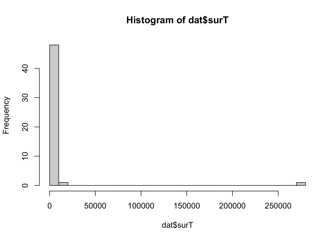

Past versions of unnamed-chunk-4-1.png

Version	Author	Date
d1c8e37	yunqiyang0215	2023-02-05

## Add survival object. status == 2 is death
dat$SurvObj <- with(dat, Surv(surT, status == 2))
## Check data
head(dat)

          surT         x1         x2          x3          x4         x5
1 1.777850e-01 -0.3688273 -0.2542623 -0.03397769  1.05315805  0.1059272
2 8.033782e+03  0.8446532  0.8801352  0.37842066 -0.01565043  1.5611673
3 2.507833e-01 -1.8825864 -2.1079356  0.98607388  0.46289456  0.2286442
4 1.123710e+01  1.0117009  0.9795530  1.17174034  1.11054315 -0.4428579
5 5.339321e-03  0.4443932  0.3487988 -0.79708820 -1.38515479 -0.3536863
6 1.171557e-03  0.9869396  0.7802569  0.32268168  0.12524732 -1.4375459
          x6 status      SurvObj
1 -0.7072287      2 1.777850e-01
2  0.7678374      2 8.033782e+03
3  0.9074854      2 2.507833e-01
4 -1.9022673      2 1.123710e+01
5  0.2799462      2 5.339321e-03
6 -0.7572632      2 1.171557e-03

saveRDS(dat, "./data/sim1.rds")

Cox regression using coxph

## Fit Cox regression
res.cox <- coxph(SurvObj ~ x1 + x2 + x3 + x4 + x5 + x6, data =  dat)
res.cox

Call:
coxph(formula = SurvObj ~ x1 + x2 + x3 + x4 + x5 + x6, data = dat)

        coef exp(coef)  se(coef)      z        p
x1 -2.076160  0.125411  1.002684 -2.071   0.0384
x2 -0.480957  0.618192  0.960812 -0.501   0.6167
x3 -1.275563  0.279274  0.292328 -4.363 1.28e-05
x4 -0.364413  0.694604  0.248892 -1.464   0.1432
x5 -5.026365  0.006563  0.754415 -6.663 2.69e-11
x6 -0.190784  0.826311  0.237344 -0.804   0.4215

Likelihood ratio test=138.7  on 6 df, p=< 2.2e-16
n= 50, number of events= 50 

res.cox2 <- coxph(SurvObj ~ x2, data =  dat)
res.cox2

Call:
coxph(formula = SurvObj ~ x2, data = dat)

      coef exp(coef) se(coef)      z       p
x2 -0.6498    0.5221   0.2014 -3.227 0.00125

Likelihood ratio test=11  on 1 df, p=0.00091
n= 50, number of events= 50 

res.cox3 <- coxph(SurvObj ~ x1, data =  dat)
res.cox3

Call:
coxph(formula = SurvObj ~ x1, data = dat)

      coef exp(coef) se(coef)      z       p
x1 -0.5594    0.5715   0.2018 -2.772 0.00558

Likelihood ratio test=8.36  on 1 df, p=0.003834
n= 50, number of events= 50 

Session information

sessionInfo()

R version 4.1.1 (2021-08-10)
Platform: x86_64-apple-darwin20.6.0 (64-bit)
Running under: macOS Monterey 12.0.1

Matrix products: default
BLAS:   /usr/local/Cellar/openblas/0.3.18/lib/libopenblasp-r0.3.18.dylib
LAPACK: /usr/local/Cellar/r/4.1.1_1/lib/R/lib/libRlapack.dylib

locale:
[1] en_US.UTF-8/en_US.UTF-8/en_US.UTF-8/C/en_US.UTF-8/en_US.UTF-8

attached base packages:
[1] stats     graphics  grDevices utils     datasets  methods   base     

other attached packages:
[1] survival_3.2-11 EnvStats_2.7.0  mvtnorm_1.1-3   workflowr_1.6.2

loaded via a namespace (and not attached):
 [1] Rcpp_1.0.8.3     highr_0.9        pillar_1.6.4     compiler_4.1.1  
 [5] bslib_0.4.1      later_1.3.0      jquerylib_0.1.4  git2r_0.28.0    
 [9] tools_4.1.1      digest_0.6.28    lattice_0.20-44  jsonlite_1.7.2  
[13] evaluate_0.14    lifecycle_1.0.1  tibble_3.1.5     pkgconfig_2.0.3 
[17] rlang_1.0.6      Matrix_1.5-3     cli_3.1.0        rstudioapi_0.13 
[21] yaml_2.2.1       xfun_0.27        fastmap_1.1.0    stringr_1.4.0   
[25] knitr_1.36       fs_1.5.0         vctrs_0.3.8      sass_0.4.4      
[29] grid_4.1.1       rprojroot_2.0.2  glue_1.4.2       R6_2.5.1        
[33] fansi_0.5.0      rmarkdown_2.11   magrittr_2.0.1   whisker_0.4     
[37] splines_4.1.1    promises_1.2.0.1 ellipsis_0.3.2   htmltools_0.5.2 
[41] httpuv_1.6.3     utf8_1.2.2       stringi_1.7.5    cachem_1.0.6    
[45] crayon_1.4.1