sim_survival
Yunqi Yang
2/1/2023
Last updated: 2023-02-23
Checks: 7 0
Knit directory: survival-susie/
This reproducible R Markdown analysis was created with workflowr (version 1.6.2). The Checks tab describes the reproducibility checks that were applied when the results were created. The Past versions tab lists the development history.
Great! Since the R Markdown file has been committed to the Git repository, you know the exact version of the code that produced these results.
Great job! The global environment was empty. Objects defined in the global environment can affect the analysis in your R Markdown file in unknown ways. For reproduciblity it’s best to always run the code in an empty environment.
The command set.seed(20230201) was run prior to running the code in the R Markdown file. Setting a seed ensures that any results that rely on randomness, e.g. subsampling or permutations, are reproducible.
Great job! Recording the operating system, R version, and package versions is critical for reproducibility.
Nice! There were no cached chunks for this analysis, so you can be confident that you successfully produced the results during this run.
Great job! Using relative paths to the files within your workflowr project makes it easier to run your code on other machines.
Great! You are using Git for version control. Tracking code development and connecting the code version to the results is critical for reproducibility.
The results in this page were generated with repository version a0a62a1. See the Past versions tab to see a history of the changes made to the R Markdown and HTML files.
Note that you need to be careful to ensure that all relevant files for the analysis have been committed to Git prior to generating the results (you can use wflow_publish or wflow_git_commit). workflowr only checks the R Markdown file, but you know if there are other scripts or data files that it depends on. Below is the status of the Git repository when the results were generated:
Ignored files:
    Ignored:    .DS_Store
    Ignored:    .Rhistory
    Ignored:    .Rproj.user/
    Ignored:    analysis/.DS_Store
    Ignored:    analysis/.RData
    Ignored:    analysis/.Rhistory
    Ignored:    analysis/run_ser_simple_dat_cache/

Untracked files:
    Untracked:  analysis/ibss_null_model.Rmd

Unstaged changes:
    Modified:   analysis/check_coxph_fit.Rmd
    Deleted:    analysis/null_model_demo.Rmd
    Modified:   analysis/null_model_zscore.Rmd
    Deleted:    analysis/one_predictor_investigation.Rmd
Note that any generated files, e.g. HTML, png, CSS, etc., are not included in this status report because it is ok for generated content to have uncommitted changes.
These are the previous versions of the repository in which changes were made to the R Markdown (analysis/sim_survival.Rmd) and HTML (docs/sim_survival.html) files. If you’ve configured a remote Git repository (see ?wflow_git_remote), click on the hyperlinks in the table below to view the files as they were in that past version.
| File | Version | Author | Date | Message |
|---|---|---|---|---|
| Rmd | a0a62a1 | yunqiyang0215 | 2023-02-23 | wflow_publish("analysis/sim_survival.Rmd") |
| html | 864bb52 | yunqiyang0215 | 2023-02-12 | Build site. |
| Rmd | 13721b5 | yunqiyang0215 | 2023-02-12 | wflow_publish("analysis/sim_survival.Rmd") |
| html | 1be4f46 | yunqiyang0215 | 2023-02-12 | Build site. |
| Rmd | 8b98f20 | yunqiyang0215 | 2023-02-12 | wflow_publish("analysis/sim_survival.Rmd") |
| html | 0936904 | yunqiyang0215 | 2023-02-09 | Build site. |
| Rmd | 7ff8071 | yunqiyang0215 | 2023-02-09 | wflow_publish("analysis/sim_survival.Rmd") |
| html | 2d56706 | yunqiyang0215 | 2023-02-06 | Build site. |
| Rmd | bf1a95e | yunqiyang0215 | 2023-02-06 | wflow_publish("analysis/sim_survival.Rmd") |
| html | d1c8e37 | yunqiyang0215 | 2023-02-05 | Build site. |
| Rmd | b930826 | yunqiyang0215 | 2023-02-05 | wflow_publish("analysis/sim_survival.Rmd") |
Description:
Simulate time-to-event data based on exponential model. And fit proportional hazard model to data. Let’s first simulate data without censoring.
The exponential regression (AFT: accelerated failure time):
It assumes survival time \(T\) follows exponential distribution. Under this assumption, the hazard is constant over time. \[ \begin{split} T&\sim \exp(\mu)\\ f(t)&=\frac{1}{\mu}\exp\{-t/\mu\}\\ \lambda(t)&=1/\mu \end{split} \]
Remember in exponential distribution, \(E(T)=\mu\). So we model the \(\log\mu\) part by linear combinations of variables. \[ \begin{split} \log(T_i) &= \log(E(T_i)) + \epsilon_i\\ &=\beta_0 + X_i^T\beta+\epsilon_i \end{split} \]
Simulate under 4 simple scenarios, 50 variables are available.
The null model, time \(T_i\) is simulated from the model that only has intercept. High correlation among all predictors.
Single effect model without correlation. Time \(T_i\) depends on \(x_1\) only, and no correlation between \(x_1\) and other variables.
Single effect model with correlation. Time \(T_i\) depends on \(x_1\) only, and high correlation between \(x_1\) and other variables.
\(\log T_i = \beta_0+\beta_1x_{i1} + \beta_2x_{i2}+\epsilon_i\), and high correlation among all variables.
library(mvtnorm)
library(survival)
# Function to construct correlation matrix among predictors.
# Diagonal elements are all 1s, the off-diagonal elements = corr
# @param p: number of predictors
# @param corr: correlation
cov_simple_het = function(p, corr){
for(i in 1:length(corr)){
cov = matrix(corr, nrow=p,ncol=p)
diag(cov) <- 1
}
return(cov)
}
# Here we use parametric model to simulate data with survival time,
# assuming survival time is exponentially distributed.
# We first simulate the mean of exponential from linear combinations
# of variables, and then simulate survival time.
# T\sim 1/u*exp(-t/u), and the true model is:
# log(T) = \mu + e = b0 + Xb + e
# @param b: vector of length (p+1) for true effect size, include intercept.
# @param X: variable matrix of size n by p.
# @param status: censoring status. 1 = censored, 2 = event observed.
sim_dat <- function(b, X){
n = nrow(X)
p = ncol(X)
mu <- exp(cbind(rep(1,n), X) %*% b)
surT <- rexp(n, rate = 1/mu)
dat <- data.frame(cbind(surT, X))
x.name <- unlist(lapply(1:p, function(i) paste0("x", i)))
names(dat) = c("surT", x.name)
dat$status <- rep(2, n)
return(dat)
}Scenario 1: null model, X no correlation
set.seed(1)
n <- 100
p <- 50
b <- c(1, rep(0, 50))
sigma <- cov_simple_het(p, corr = 0)
X<- rmvnorm(n, sigma = sigma)
dat1 <- sim_dat(b, X)
hist(dat1$surT, breaks = 20)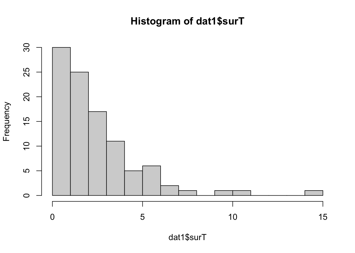
Scenario 2: null model, X correlation = 0.9
set.seed(1)
n <- 100
p <- 50
b <- c(1, rep(0, 50))
sigma <- cov_simple_het(p, corr = 0.9)
X<- rmvnorm(n, sigma = sigma)
dat2 <- sim_dat(b, X)
hist(dat2$surT, breaks = 20)
Scenario 3: single effect model with independent predictors
set.seed(1)
n <- 100
p <- 50
b <- c(1, 3, rep(0, p-1))
sigma <- cov_simple_het(p, corr = 0)
X<- rmvnorm(n, sigma = sigma)
dat3 <- sim_dat(b, X)
hist(dat2$surT, breaks = 20)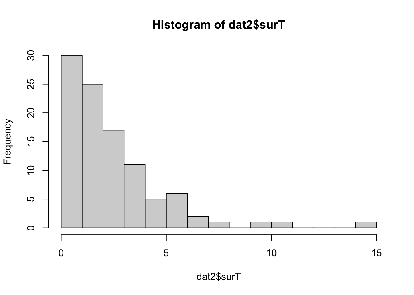
Scenario 4: single effect model with highly correlated predictors
set.seed(1)
n <- 100
p <- 50
b <- c(1, 3, rep(0, p-1))
sigma <- cov_simple_het(p, corr = 0.9)
X<- rmvnorm(n, sigma = sigma)
dat4 <- sim_dat(b, X)
hist(dat3$surT, breaks = 20)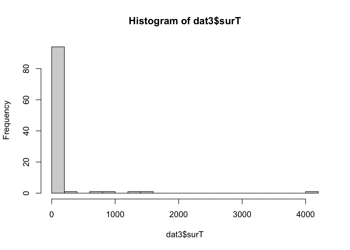
Scenario 5: two effects model with highly correlated variables
set.seed(1)
n <- 100
p <- 50
b <- c(1, 3, 1.5, rep(0, p-2))
sigma <- cov_simple_het(p, corr = 0.9)
X<- rmvnorm(n, sigma = sigma)
dat5 <- sim_dat(b, X)
hist(dat5$surT, breaks = 20)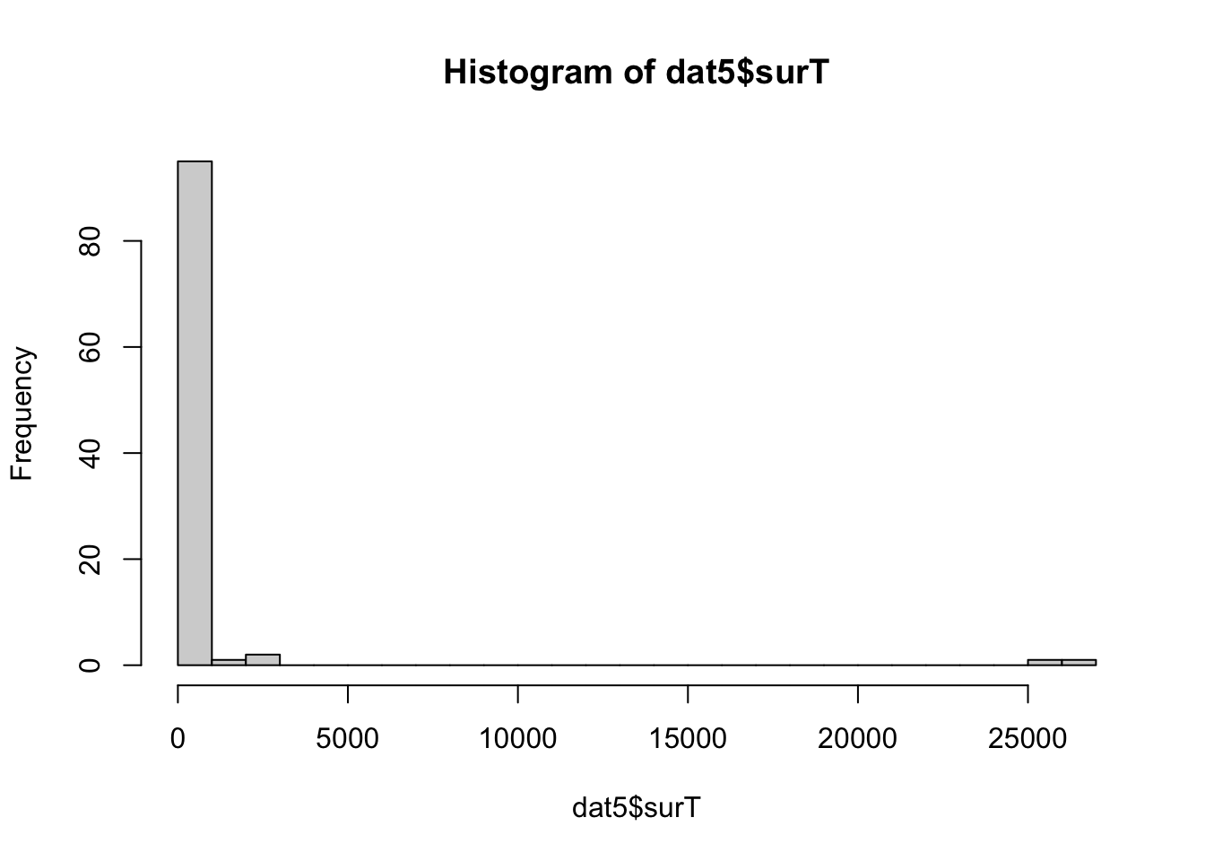
sim_dat_simple <- list(dat1, dat2, dat3, dat4, dat5)
saveRDS(sim_dat_simple, "./data/sim_dat_simple.rds")
sessionInfo()R version 4.1.1 (2021-08-10)
Platform: x86_64-apple-darwin20.6.0 (64-bit)
Running under: macOS Monterey 12.0.1
Matrix products: default
BLAS: /usr/local/Cellar/openblas/0.3.18/lib/libopenblasp-r0.3.18.dylib
LAPACK: /usr/local/Cellar/r/4.1.1_1/lib/R/lib/libRlapack.dylib
locale:
[1] en_US.UTF-8/en_US.UTF-8/en_US.UTF-8/C/en_US.UTF-8/en_US.UTF-8
attached base packages:
[1] stats graphics grDevices utils datasets methods base
other attached packages:
[1] survival_3.2-11 mvtnorm_1.1-3 workflowr_1.6.2
loaded via a namespace (and not attached):
[1] Rcpp_1.0.8.3 highr_0.9 pillar_1.6.4 compiler_4.1.1
[5] bslib_0.4.1 later_1.3.0 jquerylib_0.1.4 git2r_0.28.0
[9] tools_4.1.1 digest_0.6.28 lattice_0.20-44 jsonlite_1.7.2
[13] evaluate_0.14 lifecycle_1.0.1 tibble_3.1.5 pkgconfig_2.0.3
[17] rlang_1.0.6 Matrix_1.5-3 cli_3.1.0 rstudioapi_0.13
[21] yaml_2.2.1 xfun_0.27 fastmap_1.1.0 stringr_1.4.0
[25] knitr_1.36 fs_1.5.0 vctrs_0.3.8 sass_0.4.4
[29] grid_4.1.1 rprojroot_2.0.2 glue_1.4.2 R6_2.5.1
[33] fansi_0.5.0 rmarkdown_2.11 magrittr_2.0.1 whisker_0.4
[37] splines_4.1.1 promises_1.2.0.1 ellipsis_0.3.2 htmltools_0.5.2
[41] httpuv_1.6.3 utf8_1.2.2 stringi_1.7.5 cachem_1.0.6
[45] crayon_1.4.1