Compare PIPs: small sample + 10 iterations
Yunqi Yang
4/6/2023
Last updated: 2024-03-11
Checks: 6 1
Knit directory: survival-susie/
This reproducible R Markdown analysis was created with workflowr (version 1.7.0). The Checks tab describes the reproducibility checks that were applied when the results were created. The Past versions tab lists the development history.
Great! Since the R Markdown file has been committed to the Git repository, you know the exact version of the code that produced these results.
Great job! The global environment was empty. Objects defined in the global environment can affect the analysis in your R Markdown file in unknown ways. For reproduciblity it’s best to always run the code in an empty environment.
The command set.seed(20230201) was run prior to running
the code in the R Markdown file. Setting a seed ensures that any results
that rely on randomness, e.g. subsampling or permutations, are
reproducible.
Great job! Recording the operating system, R version, and package versions is critical for reproducibility.
Nice! There were no cached chunks for this analysis, so you can be confident that you successfully produced the results during this run.
Using absolute paths to the files within your workflowr project makes it difficult for you and others to run your code on a different machine. Change the absolute path(s) below to the suggested relative path(s) to make your code more reproducible.
| absolute | relative |
|---|---|
| /project2/mstephens/yunqiyang/surv-susie/survival-susie/code/pip.R | code/pip.R |
Great! You are using Git for version control. Tracking code development and connecting the code version to the results is critical for reproducibility.
The results in this page were generated with repository version be7519f. See the Past versions tab to see a history of the changes made to the R Markdown and HTML files.
Note that you need to be careful to ensure that all relevant files for
the analysis have been committed to Git prior to generating the results
(you can use wflow_publish or
wflow_git_commit). workflowr only checks the R Markdown
file, but you know if there are other scripts or data files that it
depends on. Below is the status of the Git repository when the results
were generated:
Ignored files:
    Ignored:    .Rproj.user/

Unstaged changes:
    Modified:   analysis/coxph_na.Rmd
Note that any generated files, e.g. HTML, png, CSS, etc., are not included in this status report because it is ok for generated content to have uncommitted changes.
These are the previous versions of the repository in which changes were
made to the R Markdown (analysis/compare_pip_10iter.Rmd)
and HTML (docs/compare_pip_10iter.html) files. If you’ve
configured a remote Git repository (see ?wflow_git_remote),
click on the hyperlinks in the table below to view the files as they
were in that past version.
| File | Version | Author | Date | Message |
|---|---|---|---|---|
| Rmd | be7519f | yunqi yang | 2024-03-11 | wflow_publish("analysis/compare_pip_10iter.Rmd") |
| html | d7d95b5 | yunqi yang | 2024-03-11 | Build site. |
| Rmd | 6189200 | yunqi yang | 2024-03-11 | wflow_publish("analysis/compare_pip_10iter.Rmd") |
| html | 422903e | yunqi yang | 2024-03-11 | Build site. |
| Rmd | a36eabb | yunqi yang | 2024-03-11 | wflow_publish("analysis/compare_pip_10iter.Rmd") |
| html | 12387fc | yunqi yang | 2024-03-11 | Build site. |
| Rmd | 8941841 | yunqi yang | 2024-03-11 | wflow_publish("analysis/compare_pip_10iter.Rmd") |
| html | c55fa8f | yunqi yang | 2024-03-11 | Build site. |
| Rmd | b4e8c1f | yunqi yang | 2024-03-11 | wflow_publish("analysis/compare_pip_10iter.Rmd") |
| html | 04c45c7 | yunqi yang | 2024-03-11 | Build site. |
| Rmd | bc79c3e | yunqi yang | 2024-03-11 | wflow_publish("analysis/compare_pip_10iter.Rmd") |
Description:
Simulation results based on real genotype data from GTEx. I took the SNPs for a certain gene, Thyroid.ENSG00000132855. Therefore, sample size \(n=584\), and I choose variable number \(p=1000\).
Steps for simulating survival data:
Select a random point on the genome, indx_start. Then the predictors are from [indx_start:(indx_start + p -1)].
Two correlation types: real correlation and independent. In independent, I simply permute each variable values. The max correlation can be 0.3, but a lot of correlation will be close to 0.
Effect size \(b\sim N(0,1)\).
Simulate survival time using exponential survival model.
Fitting:
susie: \(L=5\) and estimate prior covariance
r2b was set to default number of iterations
source("/project2/mstephens/yunqiyang/surv-susie/survival-susie/code/pip.R")susie = readRDS("/project2/mstephens/yunqiyang/surv-susie/sim2024/sim_niter10/susie.rds")
svb = readRDS("/project2/mstephens/yunqiyang/surv-susie/sim2024/sim_niter10/svb.rds")
bvsnlp = readRDS("/project2/mstephens/yunqiyang/surv-susie/sim2024/sim_niter10/bvsnlp.rds")
r2b = readRDS("/project2/mstephens/yunqiyang/surv-susie/sim2024/sim_niter10/r2b.rds")
rss = readRDS("/project2/mstephens/yunqiyang/surv-susie/sim2024/sim_niter10/rss.rds")censor_lvls = unique(susie$simulate.censor_lvl)1. Use the real correlation of SNPs
par(mfrow = c(5,4))
for (i in 1:length(censor_lvls)){
  indx = which(susie$simulate.cor_type == "real" & susie$simulate.censor_lvl == censor_lvls[i])
  pip.susie = unlist(lapply(indx, function(x) susie$susie.pip[[x]]))
  pip.svb = unlist(lapply(indx, function(x) svb$svb.pip[[x]]))
  pip.bvsnlp = unlist(lapply(indx, function(x) bvsnlp$bvsnlp.pip[[x]]))
  pip.r2b = unlist(lapply(indx, function(x) r2b$r2b.pip[[x]]))
  pip.rss = unlist(lapply(indx, function(x) rss$rss.pip[[x]]))

  is_effect = unlist(lapply(indx, function(x) susie$simulate.is_effect[[x]]))


  res.pip = compare_pip(pip.susie, pip.svb, is_effect)
  plot_pip(res.pip, labs = c("susie", "survival.svb"), main = paste0("censor=",censor_lvls[i]))
  abline(a = 0, b = 1, lty = 2, col = "blue")

  res.pip = compare_pip(pip.susie, pip.bvsnlp, is_effect)
  plot_pip(res.pip, labs = c("susie", "bvsnlp"), main = paste0("censor=",censor_lvls[i]))
  abline(a = 0, b = 1, lty = 2, col = "blue")

  res.pip = compare_pip(pip.susie, pip.r2b, is_effect)
  plot_pip(res.pip, labs = c("susie", "r2b"), main = paste0("censor=",censor_lvls[i]))
  abline(a = 0, b = 1, lty = 2, col = "blue")

  res.pip = compare_pip(pip.susie, pip.rss, is_effect)
  plot_pip(res.pip, labs = c("susie", "rss"), main = paste0("censor=",censor_lvls[i]))
  abline(a = 0, b = 1, lty = 2, col = "blue")

}
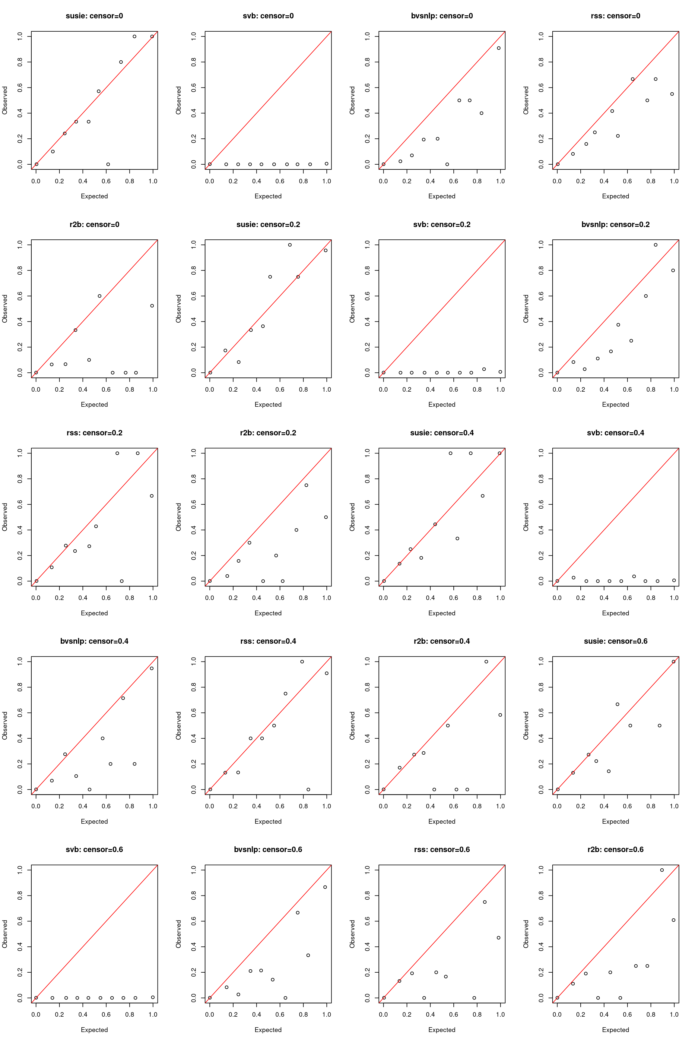
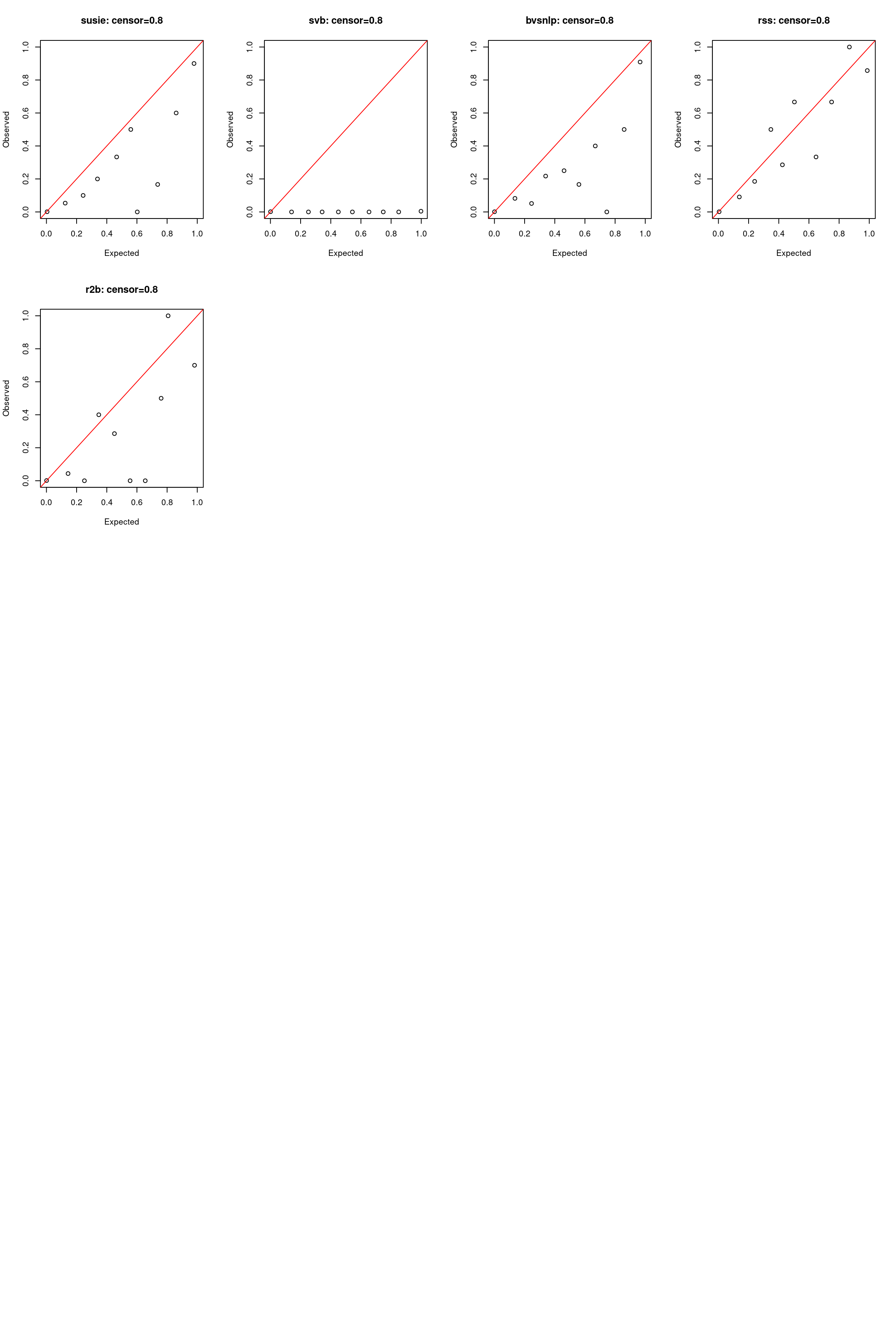
par(mfrow = c(5,4))
for (i in 1:length(censor_lvls)){
  indx = which(bvsnlp$simulate.cor_type == "real" & bvsnlp$simulate.censor_lvl == censor_lvls[i])
  is_effect = unlist(lapply(indx, function(x) bvsnlp$simulate.is_effect[[x]]))
  pip.susie = unlist(lapply(indx, function(x) susie$susie.pip[[x]]))
  pip.survsvb = unlist(lapply(indx, function(x) svb$svb.pip[[x]]))
  pip.bvsnlp = unlist(lapply(indx, function(x) bvsnlp$bvsnlp.pip[[x]]))
  pip.rss = unlist(lapply(indx, function(x) rss$rss.pip[[x]]))
  pip.r2b = unlist(lapply(indx, function(x) r2b$r2b.pip[[x]]))

  # Calibration plot for pip.susie
  calibration.susie = pip_calibration(pip.susie, is_effect)
  plot_calibration(calibration.susie, main = paste0("susie: censor=", censor_lvls[i]))

  # Calibration plot for pip.svb
  calibration.survsvb = pip_calibration(pip.survsvb, is_effect)
  plot_calibration(calibration.survsvb, main = paste0("svb: censor=", censor_lvls[i]))

  # Calibration plot for pip.bvsnlp
  calibration.bvsnlp = pip_calibration(pip.bvsnlp, is_effect)
  plot_calibration(calibration.bvsnlp, main = paste0("bvsnlp: censor=", censor_lvls[i]))

  # Calibration plot for pip.rss
  calibration.rss = pip_calibration(pip.rss, is_effect)
  plot_calibration(calibration.rss, main = paste0("rss: censor=", censor_lvls[i]))

  # Calibration plot for pip.r2b
  calibration.r2b = pip_calibration(pip.r2b, is_effect)
  plot_calibration(calibration.r2b, main = paste0("r2b: censor=", censor_lvls[i]))
}
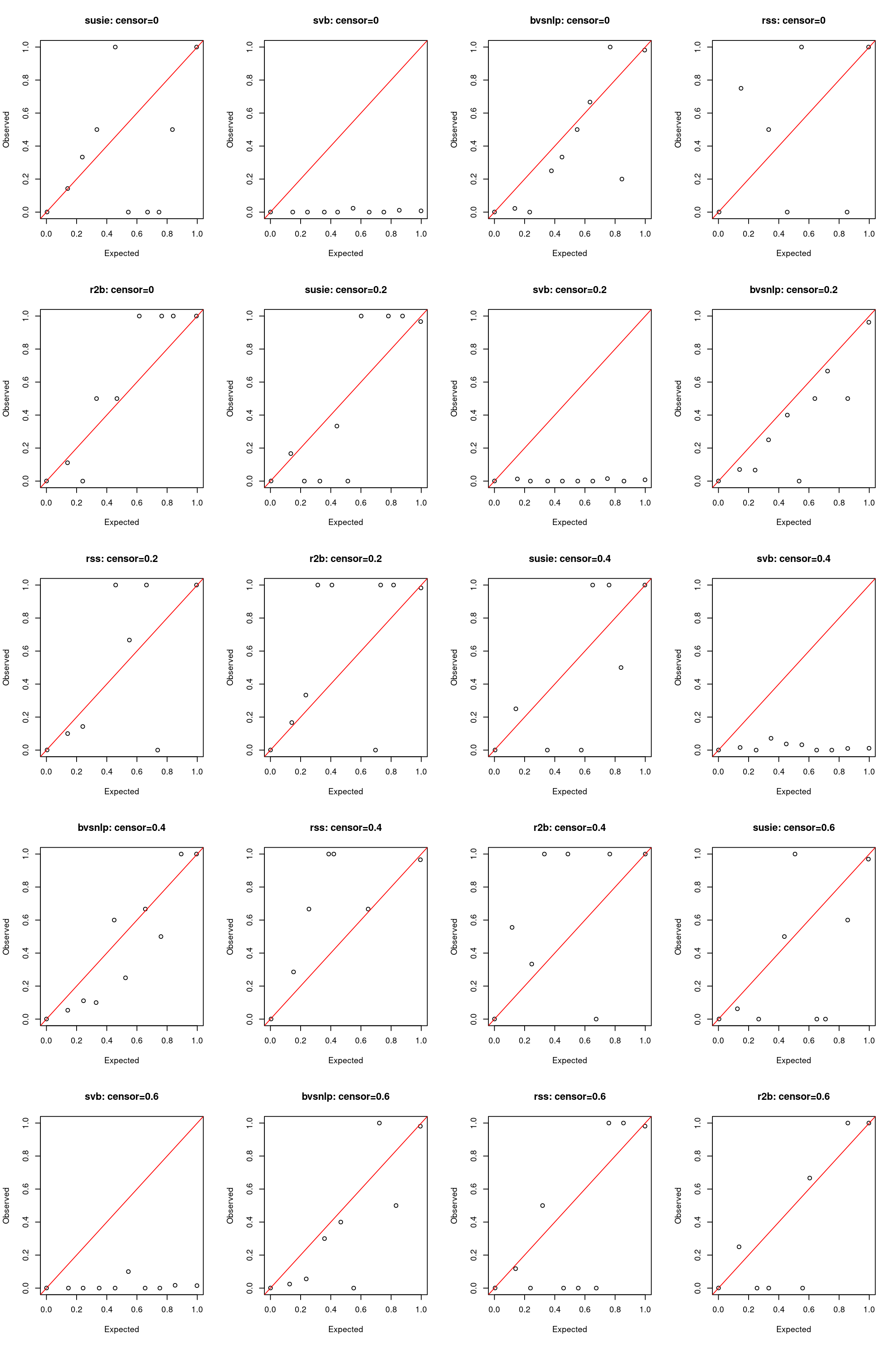
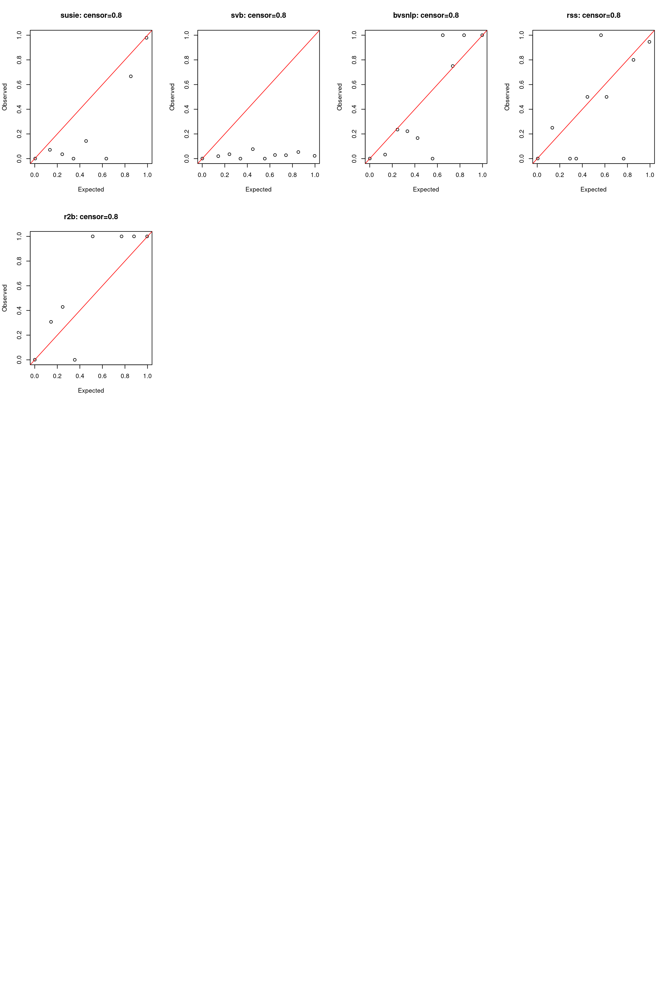
2. Near independent SNPs
par(mfrow = c(5,4))
for (i in 1:length(censor_lvls)){
  indx = which(susie$simulate.cor_type == "independent" & susie$simulate.censor_lvl == censor_lvls[i])
  pip.susie = unlist(lapply(indx, function(x) susie$susie.pip[[x]]))
  pip.svb = unlist(lapply(indx, function(x) svb$svb.pip[[x]]))
  pip.bvsnlp = unlist(lapply(indx, function(x) bvsnlp$bvsnlp.pip[[x]]))
  pip.r2b = unlist(lapply(indx, function(x) r2b$r2b.pip[[x]]))
  pip.rss = unlist(lapply(indx, function(x) rss$rss.pip[[x]]))

  is_effect = unlist(lapply(indx, function(x) susie$simulate.is_effect[[x]]))


  res.pip = compare_pip(pip.susie, pip.svb, is_effect)
  plot_pip(res.pip, labs = c("susie", "survival.svb"), main = paste0("censor=",censor_lvls[i]))
  abline(a = 0, b = 1, lty = 2, col = "blue")

  res.pip = compare_pip(pip.susie, pip.bvsnlp, is_effect)
  plot_pip(res.pip, labs = c("susie", "bvsnlp"), main = paste0("censor=",censor_lvls[i]))
  abline(a = 0, b = 1, lty = 2, col = "blue")

  res.pip = compare_pip(pip.susie, pip.r2b, is_effect)
  plot_pip(res.pip, labs = c("susie", "r2b"), main = paste0("censor=",censor_lvls[i]))
  abline(a = 0, b = 1, lty = 2, col = "blue")

  res.pip = compare_pip(pip.susie, pip.rss, is_effect)
  plot_pip(res.pip, labs = c("susie", "rss"), main = paste0("censor=",censor_lvls[i]))
  abline(a = 0, b = 1, lty = 2, col = "blue")

}
par(mfrow = c(5,4))
for (i in 1:length(censor_lvls)){
  indx = which(bvsnlp$simulate.cor_type == "independent" & bvsnlp$simulate.censor_lvl == censor_lvls[i])
  is_effect = unlist(lapply(indx, function(x) bvsnlp$simulate.is_effect[[x]]))
  pip.susie = unlist(lapply(indx, function(x) susie$susie.pip[[x]]))
  pip.survsvb = unlist(lapply(indx, function(x) svb$svb.pip[[x]]))
  pip.bvsnlp = unlist(lapply(indx, function(x) bvsnlp$bvsnlp.pip[[x]]))
  pip.rss = unlist(lapply(indx, function(x) rss$rss.pip[[x]]))
  pip.r2b = unlist(lapply(indx, function(x) r2b$r2b.pip[[x]]))

  # Calibration plot for pip.susie
  calibration.susie = pip_calibration(pip.susie, is_effect)
  plot_calibration(calibration.susie, main = paste0("susie: censor=", censor_lvls[i]))

  # Calibration plot for pip.svb
  calibration.survsvb = pip_calibration(pip.survsvb, is_effect)
  plot_calibration(calibration.survsvb, main = paste0("svb: censor=", censor_lvls[i]))

  # Calibration plot for pip.bvsnlp
  calibration.bvsnlp = pip_calibration(pip.bvsnlp, is_effect)
  plot_calibration(calibration.bvsnlp, main = paste0("bvsnlp: censor=", censor_lvls[i]))

  # Calibration plot for pip.rss
  calibration.rss = pip_calibration(pip.rss, is_effect)
  plot_calibration(calibration.rss, main = paste0("rss: censor=", censor_lvls[i]))

  # Calibration plot for pip.r2b
  calibration.r2b = pip_calibration(pip.r2b, is_effect)
  plot_calibration(calibration.r2b, main = paste0("r2b: censor=", censor_lvls[i]))
}
| Version | Author | Date |
|---|---|---|
| d7d95b5 | yunqi yang | 2024-03-11 |
| Version | Author | Date |
|---|---|---|
| d7d95b5 | yunqi yang | 2024-03-11 |
sessionInfo()
# R version 4.2.0 (2022-04-22)
# Platform: x86_64-pc-linux-gnu (64-bit)
# Running under: CentOS Linux 7 (Core)
#
# Matrix products: default
# BLAS/LAPACK: /software/openblas-0.3.13-el7-x86_64/lib/libopenblas_haswellp-r0.3.13.so
#
# locale:
#  [1] LC_CTYPE=en_US.UTF-8 LC_NUMERIC=C         LC_TIME=C
#  [4] LC_COLLATE=C         LC_MONETARY=C        LC_MESSAGES=C
#  [7] LC_PAPER=C           LC_NAME=C            LC_ADDRESS=C
# [10] LC_TELEPHONE=C       LC_MEASUREMENT=C     LC_IDENTIFICATION=C
#
# attached base packages:
# [1] stats     graphics  grDevices utils     datasets  methods   base
#
# other attached packages:
# [1] workflowr_1.7.0
#
# loaded via a namespace (and not attached):
#  [1] Rcpp_1.0.8.3     highr_0.9        bslib_0.3.1      compiler_4.2.0
#  [5] pillar_1.7.0     later_1.3.0      git2r_0.30.1     jquerylib_0.1.4
#  [9] tools_4.2.0      getPass_0.2-2    digest_0.6.29    jsonlite_1.8.0
# [13] evaluate_0.15    tibble_3.1.7     lifecycle_1.0.1  pkgconfig_2.0.3
# [17] rlang_1.0.2      cli_3.3.0        rstudioapi_0.13  yaml_2.3.5
# [21] xfun_0.30        fastmap_1.1.0    httr_1.4.3       stringr_1.4.0
# [25] knitr_1.39       sass_0.4.1       fs_1.5.2         vctrs_0.4.1
# [29] rprojroot_2.0.3  glue_1.6.2       R6_2.5.1         processx_3.8.0
# [33] fansi_1.0.3      rmarkdown_2.14   callr_3.7.3      magrittr_2.0.3
# [37] whisker_0.4      ps_1.7.0         promises_1.2.0.1 htmltools_0.5.2
# [41] ellipsis_0.3.2   httpuv_1.6.5     utf8_1.2.2       stringi_1.7.6
# [45] crayon_1.5.1