This reproducible R Markdown analysis was created with workflowr (version 1.6.2). The Checks tab describes the reproducibility checks that were applied when the results were created. The Past versions tab lists the development history.
Great job! The global environment was empty. Objects defined in the global environment can affect the analysis in your R Markdown file in unknown ways. For reproduciblity it’s best to always run the code in an empty environment.
The command set.seed(20230201) was run prior to running the code in the R Markdown file. Setting a seed ensures that any results that rely on randomness, e.g. subsampling or permutations, are reproducible.
Great! You are using Git for version control. Tracking code development and connecting the code version to the results is critical for reproducibility.
The results in this page were generated with repository version 677f671. See the Past versions tab to see a history of the changes made to the R Markdown and HTML files.
Note that you need to be careful to ensure that all relevant files for the analysis have been committed to Git prior to generating the results (you can use wflow_publish or wflow_git_commit). workflowr only checks the R Markdown file, but you know if there are other scripts or data files that it depends on. Below is the status of the Git repository when the results were generated:
Note that any generated files, e.g. HTML, png, CSS, etc., are not included in this status report because it is ok for generated content to have uncommitted changes.
These are the previous versions of the repository in which changes were made to the R Markdown (analysis/bvsnlp_censoring.Rmd) and HTML (docs/bvsnlp_censoring.html) files. If you’ve configured a remote Git repository (see ?wflow_git_remote), click on the hyperlinks in the table below to view the files as they were in that past version.
Conclusion: This method doesn’t perform well under the null model, picked one or two variables under the null model. For other 3 scenarios, it performs well.
library(survival)
library(BVSNLP)
Bayesian Variable Selection using Non-Local priors for survival and logistic regression data.
Loading Version 1.1.8
dat = readRDS("./data/sim_dat_censoring.rds")
Main function:
bvs(
  X,
  resp,
  prep = TRUE, # If preprocessing
  logT = FALSE,
  fixed_cols = NULL,
  eff_size = 0.5, # expected effect size
  family = c("logistic", "survival"),
  hselect = TRUE, # whether the automatic procedure for hyperparameter selection should be run or not.
  nlptype = "piMOM",
  r = 1,
  tau = 0.25,
  niter = 30,
  mod_prior = c("unif", "beta"),
  inseed = NULL,
  cplng = FALSE, # This parameter is only used in logistic regression models
  ncpu = 4,
  parallel.MPI = FALSE
)
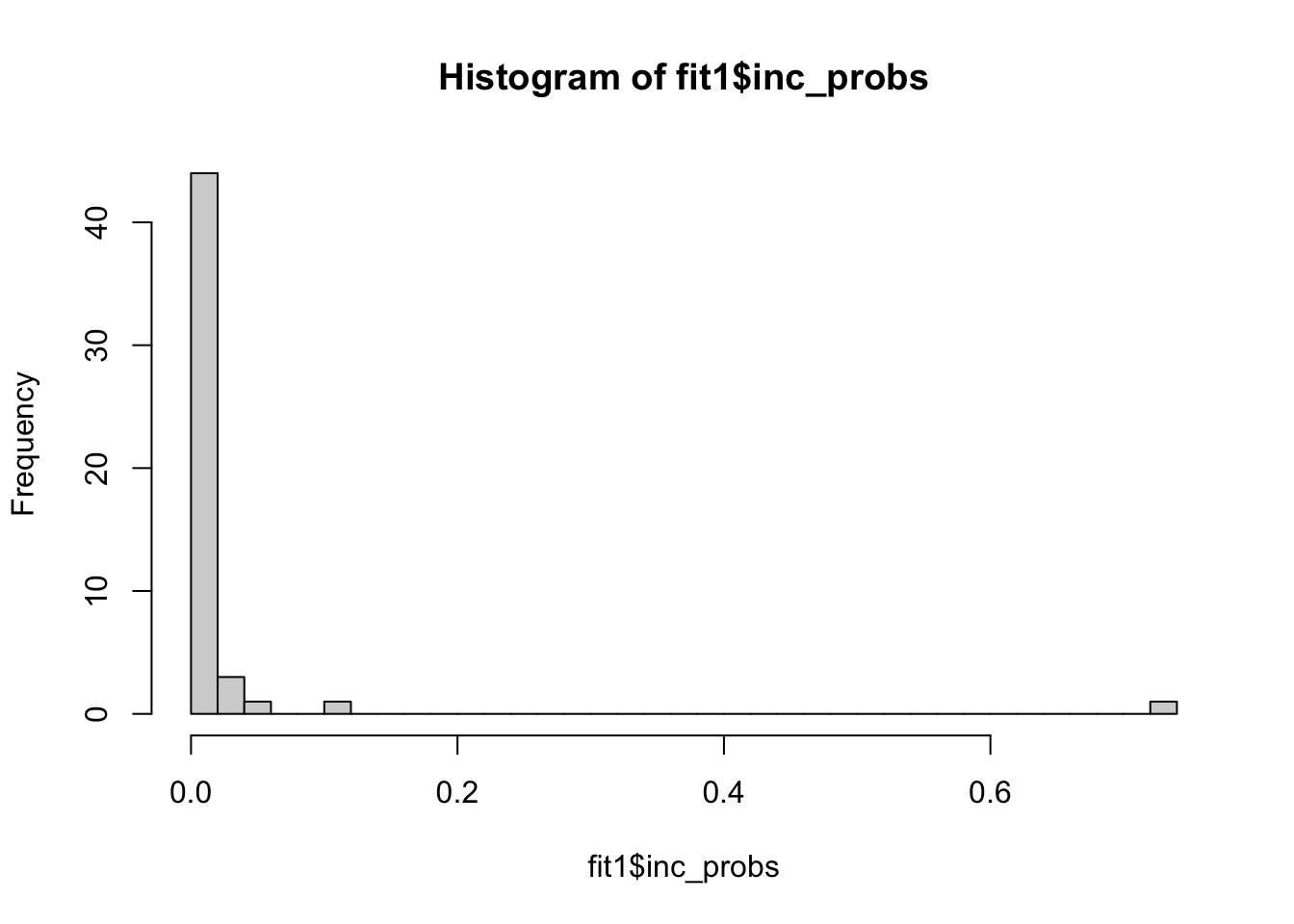
Data 1: null model with X independent
# Create survival response
dat[[1]]$y <- with(dat[[1]], Surv(surT, status))

p = 50
X = as.data.frame(dat[[1]][, c(2:(p+1))])
y = dat[[1]]$y
# prep: standardizing non-binary columns and adding intercept
fit1 = bvs(X, resp = y, prep = TRUE, family = "survival", mod_prior = "unif", niter = 100)
# The coefficient vector for the selected model.
# The first component is always for the intercept.
fit1$beta_hat
[1] -0.416437
# The indices of the model with highest posterior probability among all visited
# models, with respect to the columns in the output des_mat.
fit1$HPM
     [,1]
[1,]    4
hist(fit1$inc_probs, breaks = 30)
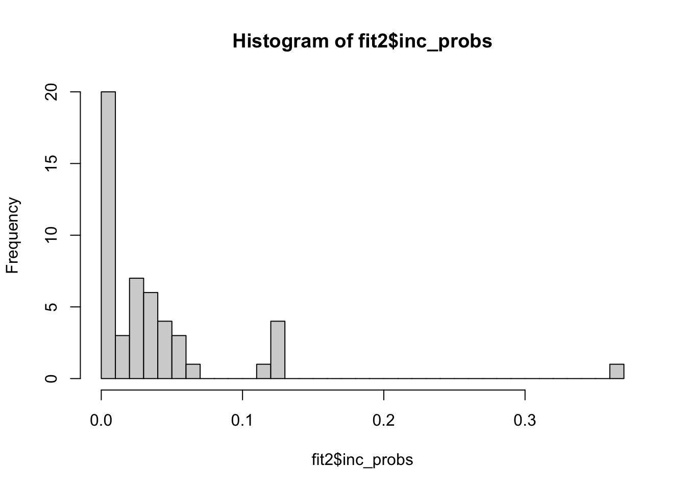
Data 2: simulated from null model with highly correlated X. corr = 0.9
# Create survival response
dat[[2]]$y <- with(dat[[2]], Surv(surT, status))
p = 50
X = as.data.frame(dat[[2]][, c(2:(p+1))])
y = dat[[2]]$y
fit2 = bvs(X, resp = y, prep = TRUE, family = "survival", mod_prior = "unif", niter = 100)
fit2$beta_hat
[1] -0.6468299 0.7292075
fit2$HPM
     [,1]
[1,]    4
[2,]    7
hist(fit2$inc_probs, breaks = 30)
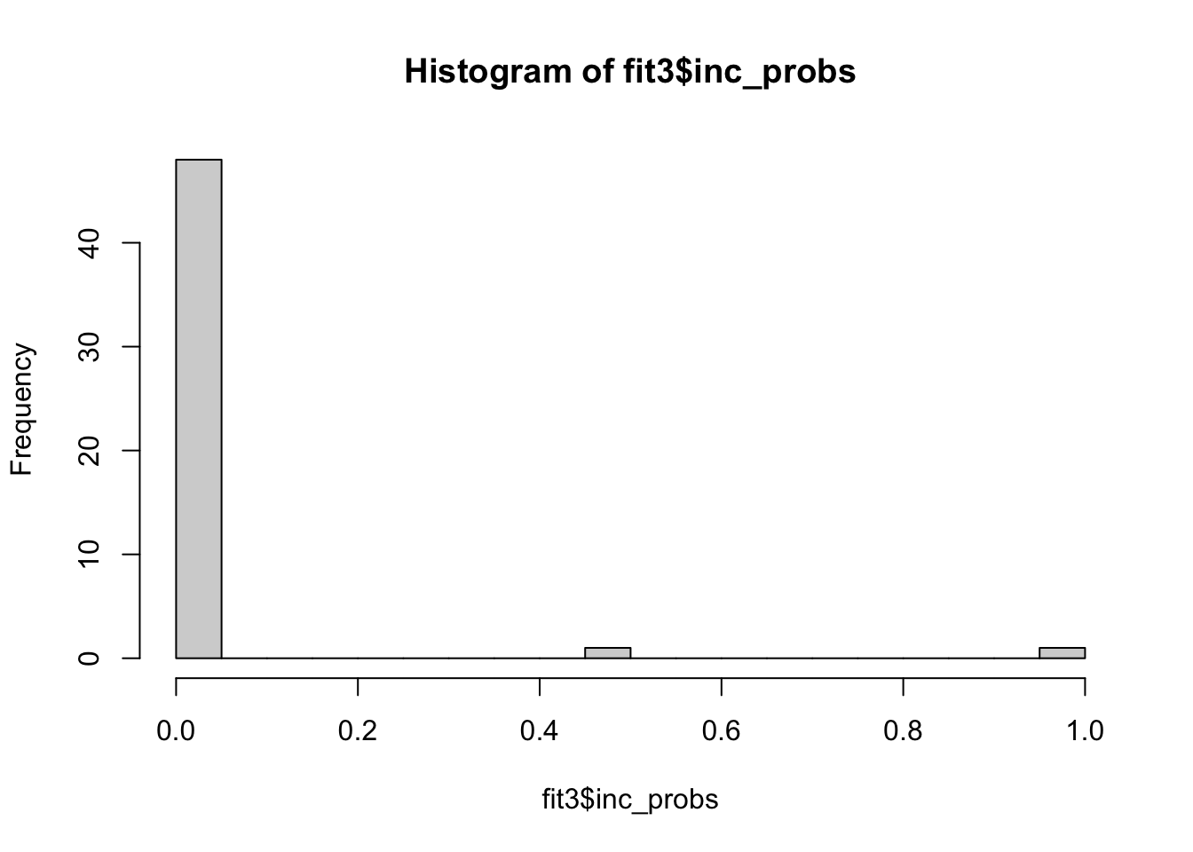
Data 3: simulated from one predictor model. Predictors are independent.
# Create survival response
dat[[3]]$y <- with(dat[[3]], Surv(surT, status))

p = 50
X = as.data.frame(dat[[3]][, c(2:(p+1))])
y = dat[[3]]$y
fit3 = bvs(X, resp = y, prep = TRUE, family = "survival", mod_prior = "unif", niter = 100)
fit3$beta_hat
[1] -3.600575
fit3$HPM
     [,1]
[1,]    1
hist(fit3$inc_probs, breaks = 30)
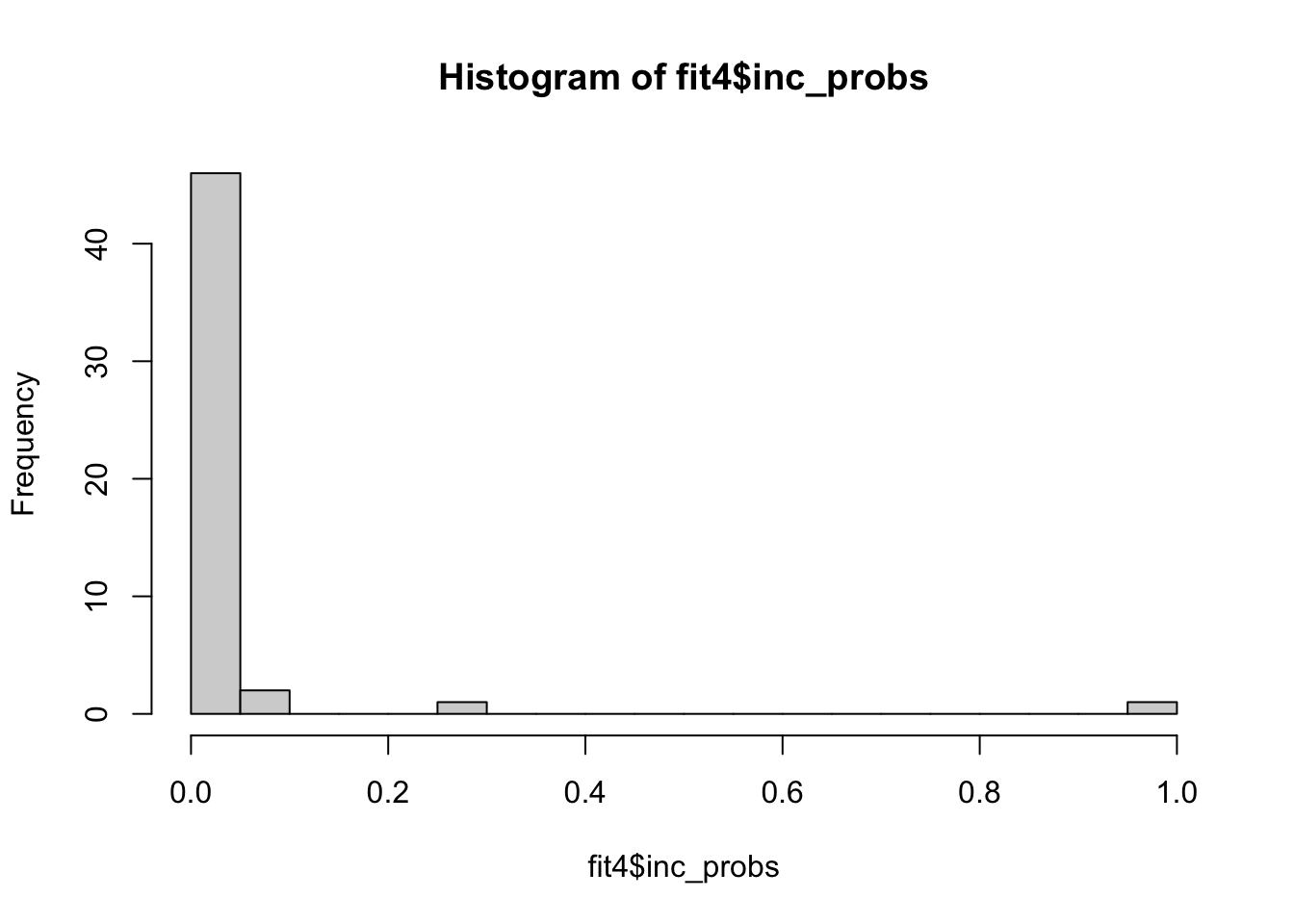
Data 4: simulated from one predictor model. Predictors are highly correlated, corr = 0.9
# Create survival response
dat[[4]]$y <- with(dat[[4]], Surv(surT, status))

p = 50
X = as.data.frame(dat[[4]][, c(2:(p+1))])
y = dat[[4]]$y
fit4 = bvs(X, resp = y, prep = TRUE, family = "survival", mod_prior = "unif", niter = 100)
fit4$beta_hat
[1] -3.254939
fit4$HPM
     [,1]
[1,]    1
hist(fit4$inc_probs, breaks = 30)
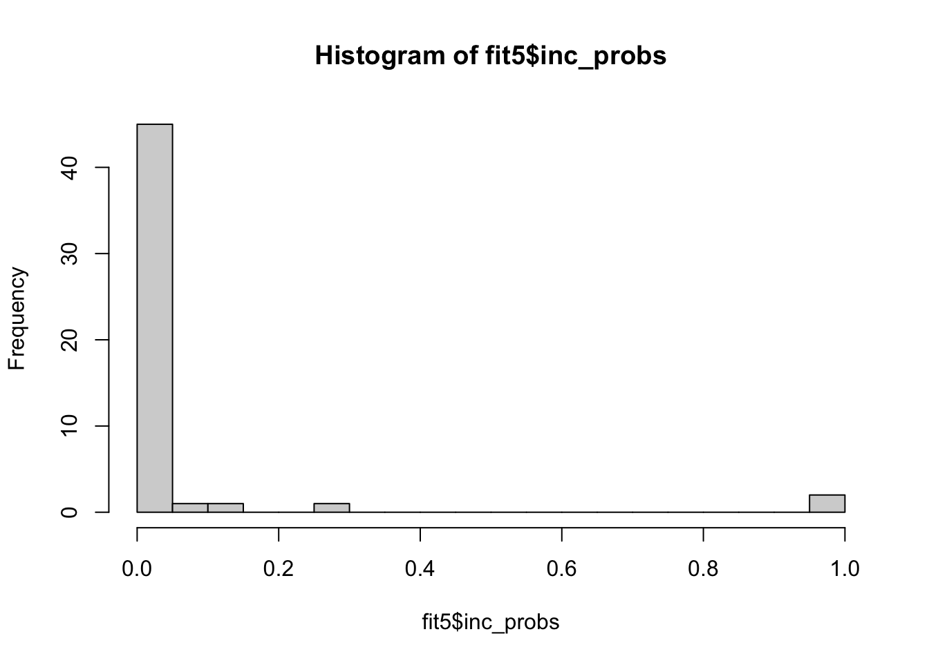
Data 5: simulated from two predictor model. Predictors have high correlation, corr = 0.9
# Create survival response
dat[[5]]$y <- with(dat[[5]], Surv(surT, status))

p = 50
X = as.data.frame(dat[[5]][, c(2:(p+1))])
y = dat[[5]]$y
fit5 = bvs(X, resp = y, prep = TRUE, family = "survival", mod_prior = "unif", niter = 100)