Last updated: 2022-06-08

Checks: 7 0

Knit directory: BASS-analysis/

This reproducible R Markdown analysis was created with workflowr (version 1.7.0). The Checks tab describes the reproducibility checks that were applied when the results were created. The Past versions tab lists the development history.


Great! Since the R Markdown file has been committed to the Git repository, you know the exact version of the code that produced these results.

Great job! The global environment was empty. Objects defined in the global environment can affect the analysis in your R Markdown file in unknown ways. For reproduciblity it’s best to always run the code in an empty environment.

The command set.seed(0) was run prior to running the code in the R Markdown file. Setting a seed ensures that any results that rely on randomness, e.g. subsampling or permutations, are reproducible.

Great job! Recording the operating system, R version, and package versions is critical for reproducibility.

Nice! There were no cached chunks for this analysis, so you can be confident that you successfully produced the results during this run.

Great job! Using relative paths to the files within your workflowr project makes it easier to run your code on other machines.

Great! You are using Git for version control. Tracking code development and connecting the code version to the results is critical for reproducibility.

The results in this page were generated with repository version 90ee3a5. See the Past versions tab to see a history of the changes made to the R Markdown and HTML files.

Note that you need to be careful to ensure that all relevant files for the analysis have been committed to Git prior to generating the results (you can use wflow_publish or wflow_git_commit). workflowr only checks the R Markdown file, but you know if there are other scripts or data files that it depends on. Below is the status of the Git repository when the results were generated:


Unstaged changes:
    Modified:   data/MERFISH_Animal1.RData
    Modified:   data/starmap_mpfc.RData

Note that any generated files, e.g. HTML, png, CSS, etc., are not included in this status report because it is ok for generated content to have uncommitted changes.


These are the previous versions of the repository in which changes were made to the R Markdown (analysis/simu.Rmd) and HTML (docs/simu.html) files. If you’ve configured a remote Git repository (see ?wflow_git_remote), click on the hyperlinks in the table below to view the files as they were in that past version.

File Version Author Date Message
Rmd 90ee3a5 zhengli09 2022-06-08 Update the simulation section
html 5c699fe zhengli09 2022-03-10 Build site.
Rmd b835db9 zhengli09 2022-03-10 Add figure of additional tissue sections
html 182beeb zhengli09 2022-03-10 Build site.
Rmd 34e84d6 zhengli09 2022-03-10 Add software tutorial and multi-sample simulation
html a27dd42 zhengli09 2022-02-27 Build site.
Rmd ada7b84 zhengli09 2022-02-27 Modify links
html 9a68511 zhengli09 2022-02-27 Build site.
Rmd 4ec8df1 zhengli09 2022-02-27 Publish the introduction, simulation analysis and STARmap analysis

Introduction

This page provides code to reproduce all the simulation results for BASS. Hopefully, this can also serve as a resource for building up your simulation studies and evaluate your statistical methods.

Main simulation study

Generate simulated data

The simulation study relies on a few R packages and python softwares (e.g. SpaGCN and FICT), which need to be installed beforehand. The specific packages and all necessary functions to conduct the simulation study can be found at simulation.

source("code/simu_utils.R")
# data from STARmap (BZ5) for inferring parameters for splatter
cnts <- readRDS("data/simu_cnts.RDS")
info <- readRDS("data/simu_info.RDS")
xy <- as.matrix(info[, c("x", "y")])
starmap <- list(cnts = cnts, info = info)

# we perform 50 simulation replicates under each setting and
# the random seeds used for each replicate are generated as below
NREP <- 50
set.seed(0)
seeds <- sample(20201230, NREP)

We generate the simulated data under the baseline simulation setting. Refer to the params file for a complete list of simulation settings.

# baseline setting of all four scenarios for 
# the single tissue section analysis (L = 1)
scenarios <- 1:4 # simulation scenarios
C <- 4 # number of cell types
R <- 4 # number of spatial domains
J <- 200 # number of genes
de_prop <- 0.2 # proportion of DE genes for each cell type
de_facLoc <- 1.1 # DE gene strength
L <- 1 # number of tissue sections

# illustrate the data at the first replicate
rep <- 1
sim_dats <- lapply(scenarios, function(scenario){
  simu(starmap = starmap, scenario = scenario, C = C, J = J, L = L, 
    batch_facLoc = 0, de_prop = de_prop, de_facLoc = de_facLoc, 
    de_facScale = 0.4, sim_seed = seeds[rep], debug = FALSE)
})
# The simulated data include an L-list of gene expression count matrices,
# an L-list of true cell type label vectors for evaluation purpose, and 
# the random seed used for generating the data
scenario <- 3
sim_dat <- sim_dats[[scenario]]
# gene expression count matrix of the first tissue section under scenario 3
sim_dat[[1]][[1]][1:5, 1:5]
      Cell1 Cell2 Cell3 Cell4 Cell5
Gene1     0     0     0     0     0
Gene2    17     2     6     9     1
Gene3     0     0     0     0     0
Gene4     0     0     0     0    19
Gene5     0     1     3     0    44

Visualize the simulated data

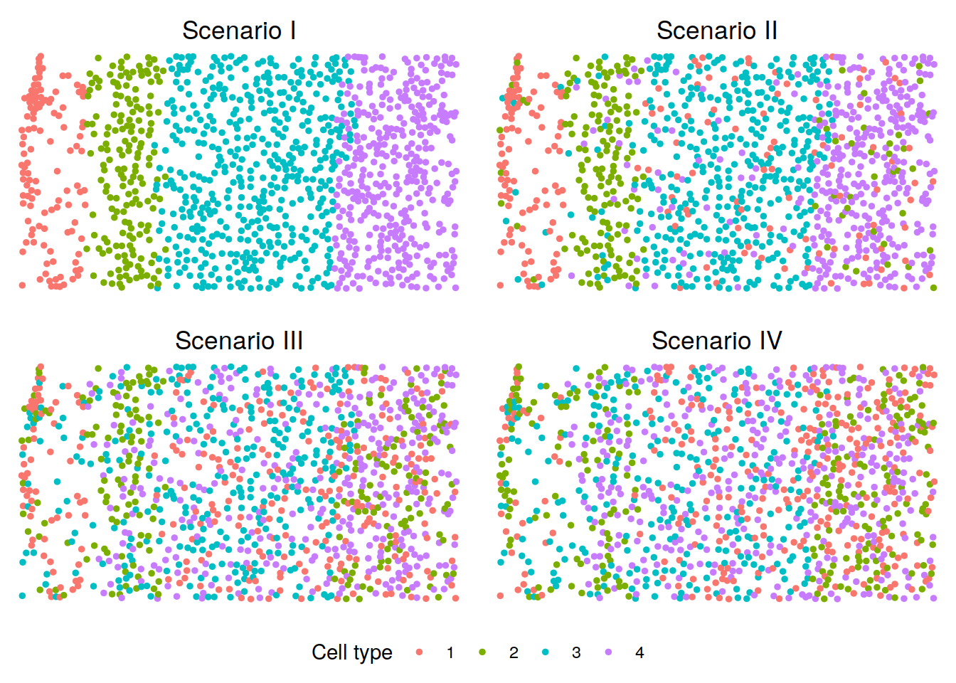
We visualize the cell type distributions under scenarios I-IV. You can refer to visualization for some useful plotting functions or you can write your own code for plotting.

library(cowplot)
source("code/viz.R")
p <- lapply(scenarios, function(scenario){
  plotClusters(xy, labels = sim_dats[[scenario]][[2]][[1]], 
    title = paste("Scenario", c("I", "II", "III", "IV")[scenario]))
})
legend <- get_legend(p[[1]] + 
  theme(legend.position = "bottom") +
  guides(color = guide_legend(title = "Cell type")))
p <- plot_grid(plotlist = p, ncol = 2)
plot_grid(p, legend, ncol = 1, rel_heights = c(1, 0.1))
Version Author Date
182beeb zhengli09 2022-03-10
9a68511 zhengli09 2022-02-27

Running all methods

We have wrapped up code for running different methods into different functions. Those functions take in simulated data and output various evaluation quantities that include the adjusted random index (ARI), \(F_1\) score, Matthew’s correlation coefficient (MCC), estimated number of cell types/spatial domains, and proportions of cells in each cell type/spatial domain. There, ARI, which was used as a major evaluation metric in our study, measures the similarity between the estimated cell type/spatial domain labels and the underlying truth. Functions for running different methods can be found at simulation. We take the simulated data from scenario 3 as an example to illustrate running different methods.

scenario <- 3

Run BASS

BASS_out <- run_BASS(sim_dats[[scenario]], xy, "SW", 
  beta = 1, C, R, init_method = "kmeans")
***************************************
  INPUT INFO:
    - Number of tissue sections: 1 
    - Number of cells/spots: 1127 
    - Number of genes: 200 
    - Potts interaction parameter estimation method: SW 
      - Estimate Potts interaction parameter with SW algorithm
  To list all hyper-parameters, Type listAllHyper(BASS_object)
***************************************
***** Log-normalize gene expression data *****
***** Exclude genes with 0 expression *****
***** Reduce data dimension with PCA *****
Post-processing...
done

Note that for cell type clustering, we evaluate three metrics that include the ARI, \(F_1\)-score, and MCC. The three metrics are evaluated in all cells, cells of major types, and cells of rare types. In our main simulation study, we focus on the ARI evaluated in all cells. The other quantities are relevant to the additional simulation studies where we evaluate the influence of rare cell types on the performance of all methods. Refer to the simulation section of our paper for details.

BASS_out
$c_ari
  all_ari major_ari  rare_ari 
0.9695299 0.9695299       NaN 

$c_F1
   all_F1  major_F1   rare_F1 
0.9882687 0.9882687        NA 

$c_MCC
  all_MCC major_MCC  rare_MCC 
0.9844597 0.9844597        NA 

$C_est
[1] 4

$c_clust_prop
[1] "0.247559893522626,0.176574977817214,0.273291925465839,0.302573203194321"

$z_ari
[1] 0.9218507

$R_est
[1] 4

$z_clust_prop
[1] "0.109139307897072,0.149068322981366,0.42413487133984,0.317657497781721"

$pi_est
          [,1]        [,2]      [,3]      [,4]
[1,] 0.5203252 0.005952381 0.2635983 0.2458101
[2,] 0.2032520 0.488095238 0.0000000 0.2569832
[3,] 0.2764228 0.255952381 0.4832636 0.0000000
[4,] 0.0000000 0.250000000 0.2531381 0.4972067

$mse_pi
[1] 0.04320112

$beta
[1] 1.095881

Run HMRF

Please note that running HMRF requires you to specify a path to python and will generate intermediate and final results into a specified folder. Please modify those directories accordingly in the run_HMRF function if you want to use the function for your own analysis.

# Note that case and rep parameters below are used to generate 
# a unique temporary directories for running HMRF.
HMRF_out <- run_HMRF(sim_dat, xy, ztrue = info$z, R, case = 3, 
  rep, usePCs = F, dosearchSEgenes = T)
# ARI for spatial domain detection across different
# spatial interaction parameter betas.
unlist(HMRF_out$ari)
      0.0       2.0       4.0       6.0       8.0      10.0      12.0      14.0 
0.1368218 0.1398503 0.1466260 0.1940655 0.2727412 0.3260866 0.4170812 0.4131667 
     16.0      18.0      20.0      22.0      24.0      26.0      28.0      30.0 
0.4472270 0.4866415 0.5182837 0.5387182 0.5534947 0.5357085 0.5570362 0.5562740 
     32.0      34.0      36.0      38.0      40.0      42.0      44.0      46.0 
0.5312894 0.5347619 0.5264228 0.5483099 0.5130628 0.5501064 0.5577595 0.5512178 
     48.0      50.0 
0.5621996 0.5594036 

Run BayesSpace

Note that BayesSpace cannot identify any neighbors because it was developed for analyzing ordered lattice structure of spots from ST or 10x Visium platform.

BayesSpace_out <- run_BayesSpace(sim_dat, xy, ztrue = info$z, R)
Neighbors were identified for 0 out of 1127 spots.
Fitting model...
Calculating labels using iterations 1000 through 10000.
# ARI for spatial domain detection, estimated number of domains,
# and proportions of cells in each domain
BayesSpace_out
$ari
[1] 0.1515157

$R_est
[1] 4

$z_clust_prop
[1] "0.254658385093168,0.177462289263531,0.26885536823425,0.299023957409051"

Run SpaGCN

Because SpaGCN was originally developed with Python, we wrapped up the python code into a function and have it imported into R such that we can conveniently analyze the simulated data in R. The python function can be found at simulation.

source_python("code/run_SpaGCN.py")
SpaGCN_out <- run_SpaGCN(sim_dat, xy, info$z, R)
# ARI for spatial domain detection, estimated number of domains,
# and proportions of cells in each domain
SpaGCN_out
$ari
[1] 0.2346377

$R_est
[1] 4

$z_clust_prop
[1] "0.215616681455191,0.186335403726708,0.29547471162378,0.302573203194321"

Run Seurat

Because Seurat uses a resolution parameter to indirectly determine the number of clusters, we run Seurat on a range of resolution parameters and identify the first value that resulted in the desired number of cell types.

resolutions <- seq(0.1, 4, by = 0.1)
seu_out <- seu_cluster(sim_dat, C, resolutions)
# ARI, F1-score, and MCC for cell type clustering, 
# number of identified clusters, and the proportion 
# of cells in each cell type cluster.
seu_out
$metric
  all_ari major_ari  rare_ari    all_F1  major_F1   rare_F1   all_MCC major_MCC 
0.9308230 0.9308230       NaN 0.9726765 0.9726765        NA 0.9638171 0.9638171 
 rare_MCC 
       NA 

$C_est
[1] 4

$clust_props
[1] "0.248447204968944,0.173025732031943,0.270629991126886,0.307897071872227"

Run SC3

Note that when the number of cells exceeds 5,000, SC3 randomly selects 5,000 cells for clustering, trains a support vector machine with the cluster labels obtained from the 5,000 cells, and then predict the cluster labels of the remaining cells.

# Note that SC3 is slow
sc3_out <- sc3_cluster(sim_dat, C)
Setting SC3 parameters...
Calculating distances between the cells...
Performing transformations and calculating eigenvectors...
Performing k-means clustering...
Calculating consensus matrix...
# ARI, F1-score, and MCC for cell type clustering, 
# number of identified clusters, and the proportion 
# of cells in each cell type cluster.
sc3_out
$metric
  all_ari major_ari  rare_ari    all_F1  major_F1   rare_F1   all_MCC major_MCC 
0.9602983 0.9602983       NaN 0.9845671 0.9845671        NA 0.9795533 0.9795533 
 rare_MCC 
       NA 

$C_est
[1] 4

$clust_props
[1] "0.249334516415262,0.179236912156167,0.267080745341615,0.304347826086957"

Run FICT

Please install the software according to the FICT github and modify the paths to the FICT software and a temporary folder accordingly in the fict_cluster function.

# Note that case and rep parameters below are used to generate 
# a unique temporary directories for running FICT.
fict_out <- fict_cluster(sim_dat, xy, C, case = 3, rep)
# ARI, F1-score, and MCC for cell type clustering, 
# number of identified clusters, and the proportion 
# of cells in each cell type cluster.
fict_out
$metric
  all_ari major_ari  rare_ari    all_F1  major_F1   rare_F1   all_MCC major_MCC 
0.9566095 0.9566095       NaN 0.9823905 0.9823905        NA 0.9768416 0.9768416 
 rare_MCC 
       NA 

$C_est
[1] 4

$clust_props
[1] "0.245785270629991,0.184560780834073,0.267080745341615,0.302573203194321"
Multi-sample simulation

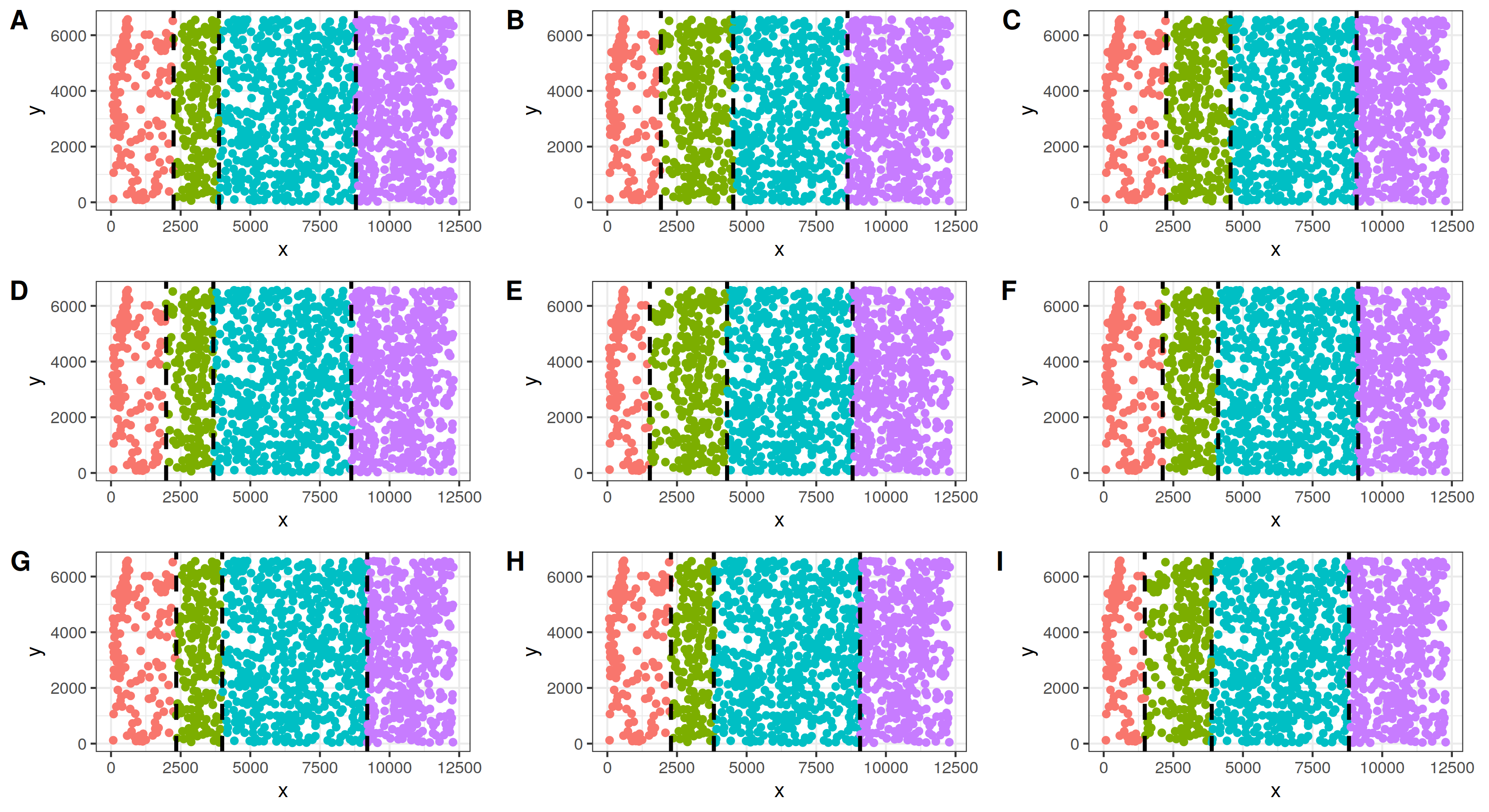
In addition to simulating and analyzing a single tissue section, we also simulated multiple tissue sections and evaluated the performance of BASS for multi-sample integrative analysis. Specifically, we generated additional tissue sections based on the same spatial locations of the 1,127 cells in the single tissue section analysis but with slightly different spatial domain allocations for them, creating varying spatial domain boundaries between the four cortical layers on different tissue sections. In each section, we set the spatial domain boundaries to be vertical, and created new boundaries by horizontally moving the original boundaries based on a uniform distribution with step size set to be approximately 10% (= 500) of the tissue width. The resulting new tissue sections are as follows.

Here, similar to the single-sample analysis, we generate the simulated data under the baseline simulation setting but for five tissue sections (L = 5). Refer to the params_mult file for a complete list of simulation settings.

# generate simulated data for five tissue sections
L <- 5
sim_dat <- simu(
  starmap = starmap, scenario = scenario, C = C, J = J, L = L, 
  batch_facLoc = 0, de_prop = de_prop, de_facLoc = de_facLoc, 
  de_facScale = 0.4, sim_seed = seeds[rep], debug = FALSE)
# run BASS
BASS_out <- run_BASS(sim_dat, xy, "SW", beta = 1, 
  C, R, init_method = "kmeans")
***************************************
  INPUT INFO:
    - Number of tissue sections: 5 
    - Number of cells/spots: 1127 1127 1127 1127 1127 
    - Number of genes: 200 
    - Potts interaction parameter estimation method: SW 
      - Estimate Potts interaction parameter with SW algorithm
  To list all hyper-parameters, Type listAllHyper(BASS_object)
***************************************
***** Log-normalize gene expression data *****
***** Exclude genes with 0 expression *****
***** Reduce data dimension with PCA *****
***** Correct batch effect with Harmony *****
Post-processing...
done
BASS_out
$c_ari
  all_ari major_ari  rare_ari 
0.9641914 0.9641914       NaN 

$c_F1
   all_F1  major_F1   rare_F1 
0.9857277 0.9857277        NA 

$c_MCC
  all_MCC major_MCC  rare_MCC 
0.9811072 0.9811072        NA 

$C_est
[1] 4

$c_clust_prop
[1] "0.242945874001775,0.196628216503993,0.246850044365572,0.31357586512866"

$z_ari
[1] 0.9292019

$R_est
[1] 4

$z_clust_prop
[1] "0.111978704525288,0.156699201419698,0.372670807453416,0.358651286601597"

$pi_est
          [,1]        [,2]      [,3]        [,4]
[1,] 0.5182250 0.001132503 0.2538095 0.251360713
[2,] 0.2662441 0.505096263 0.0000000 0.244433449
[3,] 0.2155309 0.234428086 0.4976190 0.001484414
[4,] 0.0000000 0.259343148 0.2485714 0.502721425

$mse_pi
[1] 0.01284252

$beta
[1] 1.106375

Additional simulations

Besides the main simulations above, we also performed additional simulations to evaluate the influence of various other factors – including the specified number of cell types and spatial domains, rare cell types, and a random exclusion of genes – on method performance. Please check the simulation section of our paper for detailed description of the simulation design. A list of simulation settings and code for running the simulation and for plotting can be found here. ## Influence of the specified number of cell types and spatial domains

sim_dat <- sim_dats[[scenario]]
# over-specify the number of cell types (C)
BASS_overC <- run_BASS(sim_dat, xy, "SW", beta = 1, 
  C = 10, R = 4, init_method = "kmeans")
# Note that the proportions of cells in the redundant clusters are 
# small and the spatial domain detection is only slightly affected
BASS_overC
$c_ari
  all_ari major_ari  rare_ari 
0.9333602 0.9333602       NaN 

$c_F1
   all_F1  major_F1   rare_F1 
0.9881693 0.9881693        NA 

$c_MCC
  all_MCC major_MCC  rare_MCC 
0.9842012 0.9842012        NA 

$C_est
[1] 10

$c_clust_prop
[1] "0.237799467613132,0.17036379769299,0.264418811002662,0.299023957409051,0.0115350488021295,0.0062111801242236,0.00443655723158829,0.00266193433895297,0.00266193433895297,0.000887311446317658"

$z_ari
[1] 0.9136783

$R_est
[1] 4

$z_clust_prop
[1] "0.108251996450754,0.147293700088731,0.425022182786158,0.319432120674357"

$pi_est
[1] NA

$mse_pi
[1] NA

$beta
[1] 1.1399
# over-specify the number of spatial domains (R)
BASS_overR <- run_BASS(sim_dat, xy, "SW", beta = 1, 
  C = 4, R = 10, init_method = "kmeans")
# Note that the proportions of cells in the redundant domains are 
# small and the cell type clustering is only slightly affected
BASS_overR
$c_ari
  all_ari major_ari  rare_ari 
0.9650832 0.9650832       NaN 

$c_F1
   all_F1  major_F1   rare_F1 
0.9863794 0.9863794        NA 

$c_MCC
  all_MCC major_MCC  rare_MCC 
0.9820171 0.9820171        NA 

$C_est
[1] 4

$c_clust_prop
[1] "0.249334516415262,0.175687666370896,0.273291925465839,0.301685891748004"

$z_ari
[1] 0.9177349

$R_est
[1] 6

$z_clust_prop
[1] "0.109139307897072,0.145519077196096,0.426796805678793,0.316770186335404,0.000887311446317658,0.000887311446317658"

$pi_est
[1] NA

$mse_pi
[1] NA

$beta
[1] 1.366436

Influence of rare cell types

# rare_dist = spatial/random indicates that the rare cell types 
# are either located in specific domains or distributed randomly 
# across the entire tissue section
# C = 10/14 (4 major cell types + 6/10 rare cell types)
# major cell types consist of 70% of cells in the data while
# rare cell types consist of the remaining 30% of cells
sim_dat_rare <- simu(starmap, scenario = 5, rare_dist = "spatial",
  C = 14, J = 200, L = 1, batch_facLoc = 0, de_prop = 0.2, 
  de_facLoc = 1.1, de_facScale = 0.4, sim_seed = seeds[rep])
BASS_rare <- run_BASS(sim_dat_rare, xy, "SW", beta = 1, 
  C = 14, R = 4, init_method = "kmeans")
BASS_rare
$c_ari
  all_ari major_ari  rare_ari 
0.8592284 0.9169639 0.4223043 

$c_F1
   all_F1  major_F1   rare_F1 
0.6342784 0.9567075 0.5053068 

$c_MCC
  all_MCC major_MCC  rare_MCC 
0.6357533 0.9481603 0.5107905 

$C_est
[1] 14

$c_clust_prop
[1] "0.16681455190772,0.116237799467613,0.173025732031943,0.22360248447205,0.0656610470275066,0.0372670807453416,0.0230700976042591,0.031055900621118,0.0692102928127773,0.00532386867790594,0.00443655723158829,0.0434782608695652,0.0372670807453416,0.00354924578527063"

$z_ari
[1] 0.9050962

$R_est
[1] 4

$z_clust_prop
[1] "0.108251996450754,0.153504880212955,0.417923691215617,0.320319432120674"

$pi_est
[1] NA

$mse_pi
[1] NA

$beta
[1] 1.12007

Influence of a random exclusion of genes

# I = 100, 200, or 500 indicates the number of retained genes 
# while the total number of genes is 1000 in the original gene 
# expression matrix
sim_dat_rand_excl <- simu(starmap, scenario = 3, C = 4, 
  J = 1000, I = 200, L = 1, batch_facLoc = 0, de_prop = 0.2, 
  de_facLoc = 1.1, de_facScale = 0.4, sim_seed = seeds[rep])
BASS_rand_excl <- run_BASS(sim_dat_rand_excl, xy, "SW", 
  beta = 1, C = 4, R = 4, init_method = "kmeans")
BASS_rand_excl
$c_ari
  all_ari major_ari  rare_ari 
0.7009269 0.7009269       NaN 

$c_F1
   all_F1  major_F1   rare_F1 
0.8748878 0.8748878        NA 

$c_MCC
  all_MCC major_MCC  rare_MCC 
0.8352678 0.8352678        NA 

$C_est
[1] 4

$c_clust_prop
[1] "0.247559893522626,0.193433895297249,0.246672582076309,0.312333629103815"

$z_ari
[1] 0.8896475

$R_est
[1] 4

$z_clust_prop
[1] "0.09849157054126,0.163265306122449,0.406388642413487,0.331854480922804"

$pi_est
           [,1]       [,2]        [,3]      [,4]
[1,] 0.49549550 0.02173913 0.270742358 0.2566845
[2,] 0.26126126 0.53260870 0.006550218 0.2352941
[3,] 0.22522523 0.23369565 0.458515284 0.0000000
[4,] 0.01801802 0.21195652 0.264192140 0.5080214

$mse_pi
[1] 0.1623195

$beta
[1] 1.14088

Find all the simulation results

You can find results for all the simulation studies that include the main simulation study and additional simulation studies here.


sessionInfo()
R version 4.2.0 (2022-04-22)
Platform: x86_64-pc-linux-gnu (64-bit)
Running under: Ubuntu 18.04.5 LTS

Matrix products: default
BLAS:   /usr/lib/x86_64-linux-gnu/openblas/libblas.so.3
LAPACK: /usr/lib/x86_64-linux-gnu/libopenblasp-r0.2.20.so

locale:
 [1] LC_CTYPE=en_US.UTF-8       LC_NUMERIC=C              
 [3] LC_TIME=en_US.UTF-8        LC_COLLATE=en_US.UTF-8    
 [5] LC_MONETARY=en_US.UTF-8    LC_MESSAGES=en_US.UTF-8   
 [7] LC_PAPER=en_US.UTF-8       LC_NAME=C                 
 [9] LC_ADDRESS=C               LC_TELEPHONE=C            
[11] LC_MEASUREMENT=en_US.UTF-8 LC_IDENTIFICATION=C       

attached base packages:
[1] parallel  stats4    stats     graphics  grDevices utils     datasets 
[8] methods   base     

other attached packages:
 [1] cowplot_1.1.1               CVXR_1.0-10                
 [3] reticulate_1.25             splatter_1.16.1            
 [5] gtools_3.9.2                scater_1.16.2              
 [7] forcats_0.5.0               stringr_1.4.0              
 [9] dplyr_1.0.8                 purrr_0.3.4                
[11] readr_1.3.1                 tidyr_1.1.1                
[13] tibble_3.1.6                ggplot2_3.3.5              
[15] tidyverse_1.3.0             mclust_5.4.9               
[17] GapClust_0.1.0              SC3_1.24.0                 
[19] Seurat_3.2.3                BayesSpace_1.2.1           
[21] SingleCellExperiment_1.14.1 SummarizedExperiment_1.22.0
[23] Biobase_2.48.0              GenomicRanges_1.44.0       
[25] GenomeInfoDb_1.24.2         IRanges_2.26.0             
[27] S4Vectors_0.30.2            BiocGenerics_0.38.0        
[29] MatrixGenerics_1.4.3        matrixStats_0.61.0         
[31] Giotto_1.0.4                BASS_1.1.0                 
[33] GIGrvg_0.5                  workflowr_1.7.0            

loaded via a namespace (and not attached):
  [1] rappdirs_0.3.3            scattermore_0.8          
  [3] maxLik_1.5-2              coda_0.19-4              
  [5] bit64_4.0.2               knitr_1.37               
  [7] irlba_2.3.3               DelayedArray_0.18.0      
  [9] data.table_1.14.2         rpart_4.1.16             
 [11] RCurl_1.98-1.5            doParallel_1.0.15        
 [13] generics_0.1.2            callr_3.7.0              
 [15] RSQLite_2.2.0             combinat_0.0-8           
 [17] RANN_2.6.1                proxy_0.4-26             
 [19] future_1.25.0             bit_4.0.4                
 [21] xml2_1.3.3                lubridate_1.7.9          
 [23] spatstat.data_2.2-0       httpuv_1.5.4             
 [25] assertthat_0.2.1          viridis_0.5.1            
 [27] xfun_0.29                 hms_0.5.3                
 [29] jquerylib_0.1.4           evaluate_0.15            
 [31] promises_1.1.1            DEoptimR_1.0-11          
 [33] fansi_1.0.2               readxl_1.3.1             
 [35] dbplyr_1.4.4              igraph_1.3.1             
 [37] DBI_1.1.1                 htmlwidgets_1.5.1        
 [39] Rmpfr_0.8-7               ellipsis_0.3.2           
 [41] backports_1.2.1           deldir_1.0-6             
 [43] sparseMatrixStats_1.8.0   vctrs_0.3.8              
 [45] here_0.1                  ROCR_1.0-11              
 [47] abind_1.4-5               rflann_1.5               
 [49] withr_2.4.3               cachem_1.0.6             
 [51] robustbase_0.95-0         checkmate_2.1.0          
 [53] sctransform_0.3.3         scran_1.20.1             
 [55] goftest_1.2-3             cluster_2.1.3            
 [57] lazyeval_0.2.2            Rglpk_0.6-4              
 [59] crayon_1.5.0              slam_0.1-50              
 [61] labeling_0.4.2            edgeR_3.38.0             
 [63] pkgconfig_2.0.3           nlme_3.1-157             
 [65] vipor_0.4.5               rlang_1.0.1              
 [67] globals_0.15.0            lifecycle_1.0.1          
 [69] miniUI_0.1.1.1            sandwich_3.0-1           
 [71] BiocFileCache_1.12.0      modelr_0.1.8             
 [73] rsvd_1.0.3                cellranger_1.1.0         
 [75] rprojroot_2.0.2           polyclip_1.10-0          
 [77] lmtest_0.9-40             rngtools_1.5.2           
 [79] Matrix_1.4-1              Rhdf5lib_1.10.1          
 [81] zoo_1.8-10                reprex_0.3.0             
 [83] beeswarm_0.4.0            whisker_0.4              
 [85] ggridges_0.5.3            processx_3.5.2           
 [87] pheatmap_1.0.12           png_0.1-7                
 [89] viridisLite_0.4.0         bitops_1.0-7             
 [91] getPass_0.2-2             KernSmooth_2.23-20       
 [93] blob_1.2.1                DelayedMatrixStats_1.14.3
 [95] doRNG_1.8.2               parallelly_1.31.1        
 [97] lpSolve_5.6.15            beachmat_2.8.1           
 [99] scales_1.1.1              memoise_2.0.1            
[101] magrittr_2.0.2            plyr_1.8.7               
[103] ica_1.0-2                 zlibbioc_1.34.0          
[105] DirichletReg_0.7-1        compiler_4.2.0           
[107] miscTools_0.6-26          dqrng_0.3.0              
[109] RColorBrewer_1.1-2        rrcov_1.7-0              
[111] fitdistrplus_1.1-8        cli_3.2.0                
[113] XVector_0.32.0            listenv_0.8.0            
[115] patchwork_1.1.1           pbapply_1.5-0            
[117] ps_1.6.0                  Formula_1.2-4            
[119] MASS_7.3-57               mgcv_1.8-40              
[121] tidyselect_1.1.2          stringi_1.7.6            
[123] highr_0.9                 yaml_2.3.5               
[125] BiocSingular_1.4.0        locfit_1.5-9.5           
[127] ggrepel_0.9.1             grid_4.2.0               
[129] sass_0.4.1                tools_4.2.0              
[131] future.apply_1.9.0        label.switching_1.8      
[133] rstudioapi_0.13           bluster_1.6.0            
[135] foreach_1.5.0             git2r_0.28.0             
[137] metapod_1.0.0             gridExtra_2.3            
[139] farver_2.1.0              Rtsne_0.16               
[141] digest_0.6.29             pracma_2.2.9             
[143] shiny_1.5.0               Rcpp_1.0.8.3             
[145] broom_0.7.10              scuttle_1.2.1            
[147] harmony_0.1.0             later_1.1.0.1            
[149] RcppAnnoy_0.0.19          WriteXLS_6.4.0           
[151] httr_1.4.2                Rdpack_2.3               
[153] colorspace_2.0-3          rvest_0.3.6              
[155] fs_1.5.2                  tensor_1.5               
[157] splines_4.2.0             uwot_0.1.11              
[159] statmod_1.4.36            spatstat.utils_2.3-1     
[161] xgboost_1.4.1.1           plotly_4.9.2.1           
[163] gmp_0.6-5                 xtable_1.8-4             
[165] jsonlite_1.8.0            spatstat_1.64-1          
[167] R6_2.5.1                  pillar_1.7.0             
[169] htmltools_0.5.2           mime_0.12                
[171] glue_1.6.2                fastmap_1.1.0            
[173] BiocParallel_1.22.0       BiocNeighbors_1.6.0      
[175] class_7.3-20              codetools_0.2-18         
[177] pcaPP_2.0-1               mvtnorm_1.1-3            
[179] utf8_1.2.2                lattice_0.20-45          
[181] bslib_0.3.1               curl_4.3.2               
[183] ggbeeswarm_0.6.0          leiden_0.4.2             
[185] survival_3.3-1            limma_3.52.0             
[187] rmarkdown_2.12.1          munsell_0.5.0            
[189] e1071_1.7-9               rhdf5_2.32.2             
[191] GenomeInfoDbData_1.2.6    iterators_1.0.13         
[193] smfishHmrf_0.1            haven_2.3.1              
[195] reshape2_1.4.4            gtable_0.3.0             
[197] rbibutils_2.2.8