kos_K20_ebpmf.alpha_v0.3.9
zihao12
2020-05-11
Last updated: 2020-05-16
Checks: 7 0
Knit directory: ebpmf_data_analysis/
This reproducible R Markdown analysis was created with workflowr (version 1.6.2). The Checks tab describes the reproducibility checks that were applied when the results were created. The Past versions tab lists the development history.
Great! Since the R Markdown file has been committed to the Git repository, you know the exact version of the code that produced these results.
Great job! The global environment was empty. Objects defined in the global environment can affect the analysis in your R Markdown file in unknown ways. For reproduciblity it’s best to always run the code in an empty environment.
The command set.seed(20200511) was run prior to running the code in the R Markdown file. Setting a seed ensures that any results that rely on randomness, e.g. subsampling or permutations, are reproducible.
Great job! Recording the operating system, R version, and package versions is critical for reproducibility.
Nice! There were no cached chunks for this analysis, so you can be confident that you successfully produced the results during this run.
Great job! Using relative paths to the files within your workflowr project makes it easier to run your code on other machines.
Great! You are using Git for version control. Tracking code development and connecting the code version to the results is critical for reproducibility.
The results in this page were generated with repository version 3e38a38. See the Past versions tab to see a history of the changes made to the R Markdown and HTML files.
Note that you need to be careful to ensure that all relevant files for the analysis have been committed to Git prior to generating the results (you can use wflow_publish or wflow_git_commit). workflowr only checks the R Markdown file, but you know if there are other scripts or data files that it depends on. Below is the status of the Git repository when the results were generated:
Ignored files:
    Ignored:    .Rhistory
    Ignored:    .Rproj.user/
    Ignored:    analysis/ebpmf_bg_tutorial_cache/
Note that any generated files, e.g. HTML, png, CSS, etc., are not included in this status report because it is ok for generated content to have uncommitted changes.
These are the previous versions of the repository in which changes were made to the R Markdown (analysis/kos_K20_ebpmf.alpha_v0.3.9.Rmd) and HTML (docs/kos_K20_ebpmf.alpha_v0.3.9.html) files. If you’ve configured a remote Git repository (see ?wflow_git_remote), click on the hyperlinks in the table below to view the files as they were in that past version.
| File | Version | Author | Date | Message |
|---|---|---|---|---|
| Rmd | 3e38a38 | zihao12 | 2020-05-16 | analysis for results in v0.3.9 |
Introduction
- I apply
ebpmf.alpha(version 0.3.9) to KOS dataset. I use \(K = 20\). The data has \(n = 3430,p = 6906\) and sparsity around \(98\) percent.
- Besides, I also apply to
PMF(lee’s, but I implemented a version for sparse data) to the same dataset with the same initialization. In each iteration,ebpmf_bgdoes two things: MLE for prior and updates posterior. The second part has almost the same computation as inPMF.
model
\[\begin{align} & X_{ij} = \sum_k Z_{ijk}\\ & Z_{ijk} \sim Pois(l_{i0} f_{j0} l_{ik} f_{jk})\\ & l_{ik} \sim g_{L, k}(.), f_{jk} \sim g_{F, k}(.) \end{align}\]For details see ebpmf_bg
prior options
I use gamma mixture \(\sum_l \pi_{l} Ga(1/\phi_l, 1/\phi_l)\) as prior for both \(L, F\). Note that each grid component has \(E = 1, Var = \phi_L\)
initialization
I initialized with 50 runs of NNLM::nnmf (scd). Then I used medians of each row of \(L, F\) as \(l_{i0}, f_{j0}\), and \(l_{ik} = l^0_{ik}/l_{i0}, f_{jk} = f^0_{jk}/f_{j0}\).
library(pheatmap)Warning: package 'pheatmap' was built under R version 3.5.2library(gridExtra)
source("code/misc.R")
output_dir = "output/uci_BoW/v0.3.9/"
data_dir = "data/uci_BoW/"
model_name = "kos_ebpmf_bg_initLF50_K20_maxiter5000.Rds"
model_pmf_name = "kos_pmf_initLF50_K20_maxiter5000.Rds"
dict_name = "vocab.kos.txt"
model = readRDS(sprintf("%s/%s", output_dir, model_name))
model_pmf = readRDS(sprintf("%s/%s", output_dir, model_pmf_name))
dict = read.csv(sprintf("%s/%s", data_dir, dict_name), header = FALSE)[,1]
dict = as.vector(dict)ELBO and runtime
plot(model$ELBO, xlab = "niter", ylab = "elbo")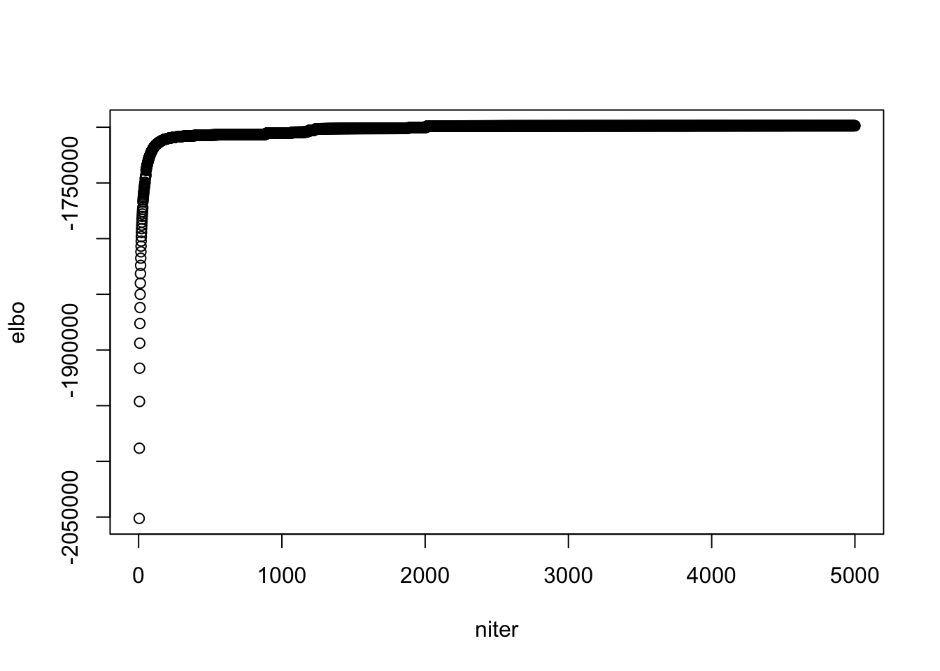
## see when it "converges"
plot(model$ELBO[1:200], xlab = "niter", ylab = "elbo")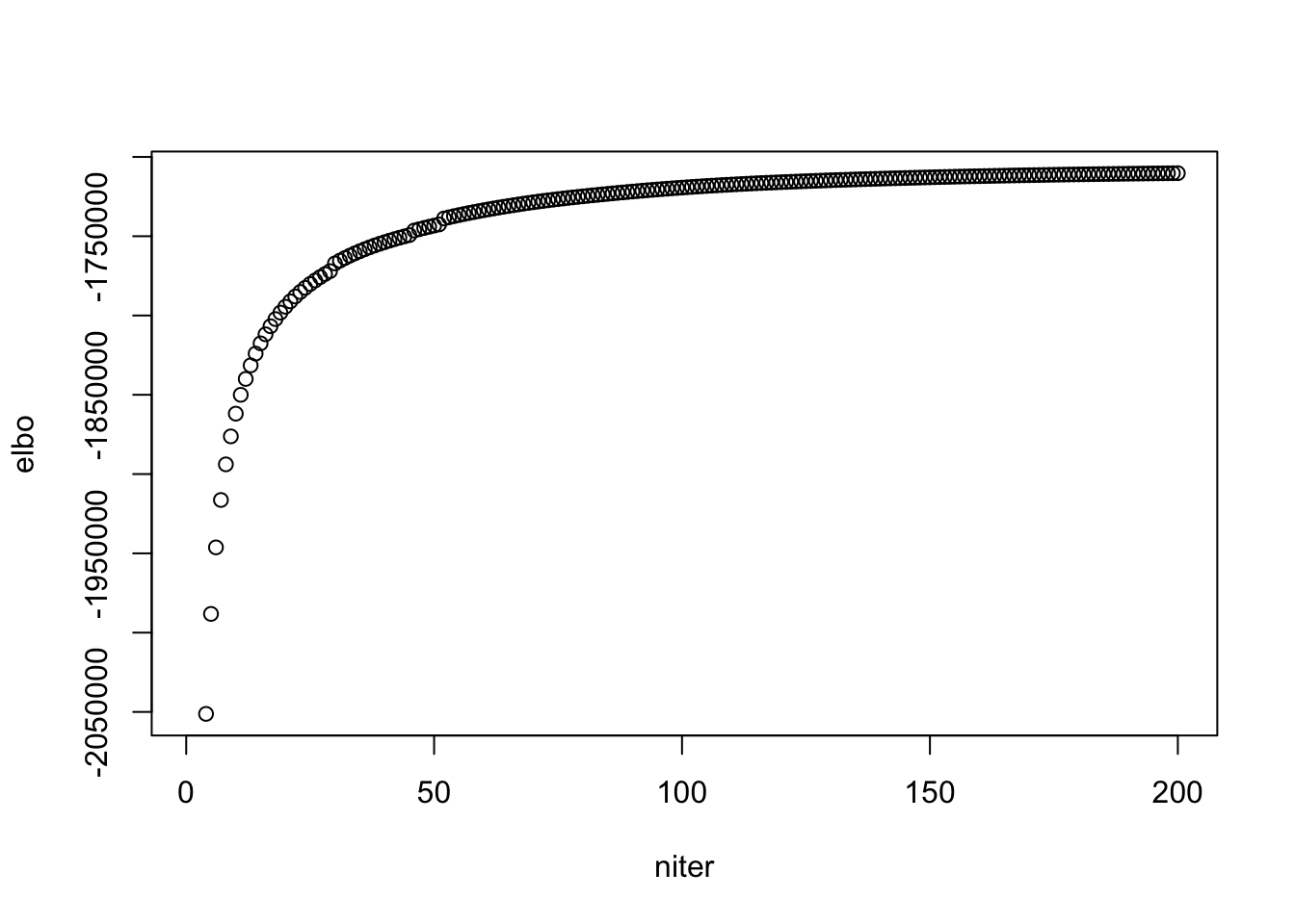
## ebpmf_bg runtime per iteration
model$runtime/length(model$ELBO)
user system elapsed
9.8347284 0.0247896 9.8627436 ## pmf runtime per iteration
model_pmf$runtime/length(model_pmf$log_liks) user system elapsed
5.0026214 0.0133454 5.0174608 look at priors in ebpmf_bg
\(g_L\)
get_prior_summary(model$qg$gls)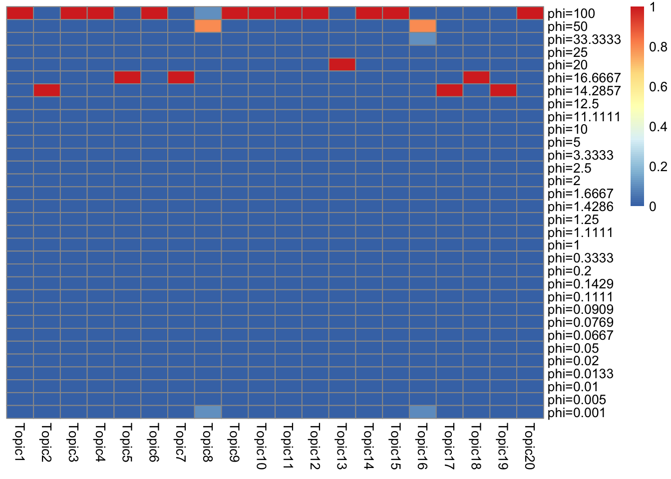
\(g_F\)
get_prior_summary(model$qg$gfs)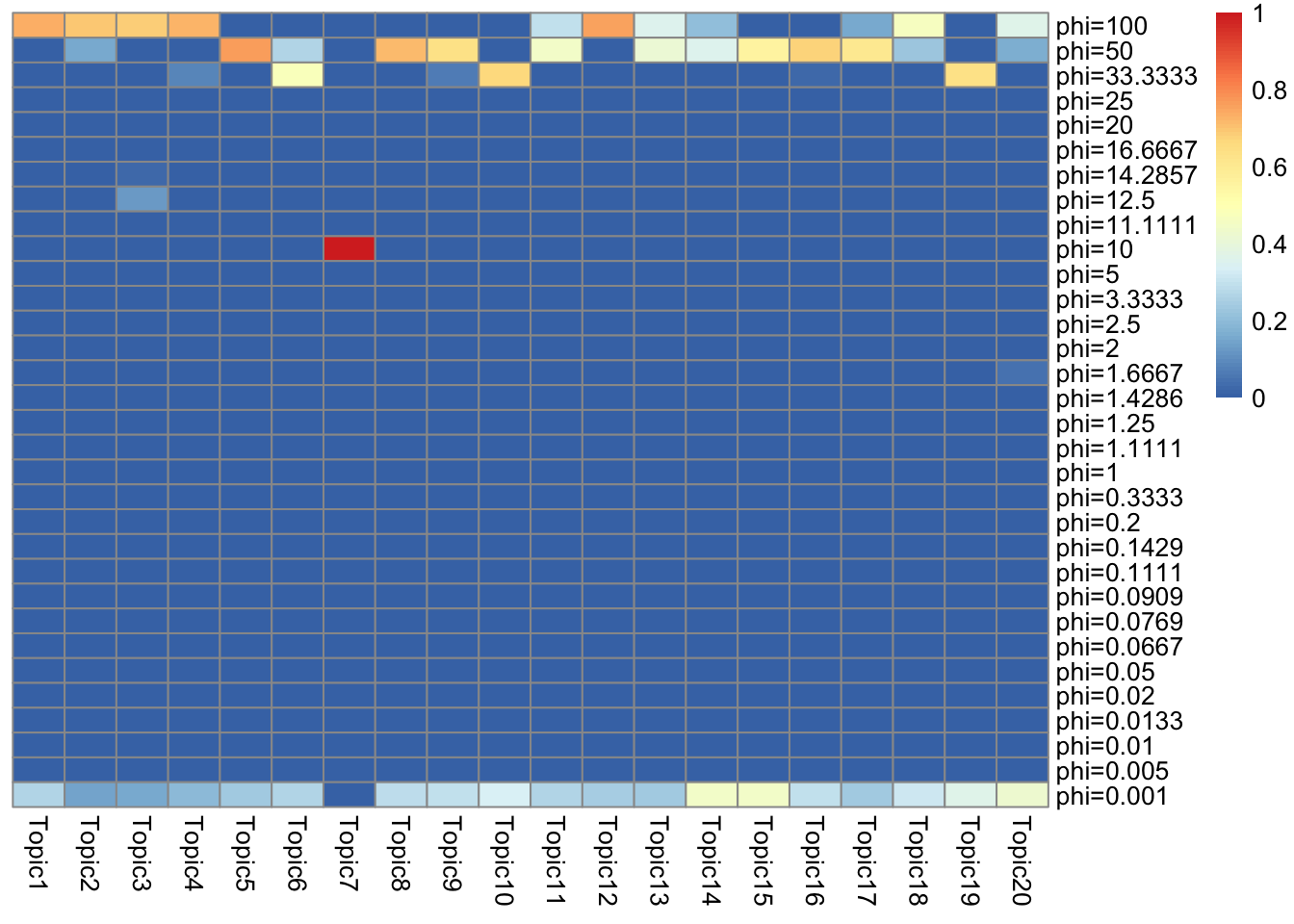
Look at quantile of topics
quantile of \(f_{J0}\) (ebpmf_bg)
f = model$f0
probs = seq(0, 1, 0.002)
plot(probs, quantile(f, probs = probs), main = sprintf("topic %d",0))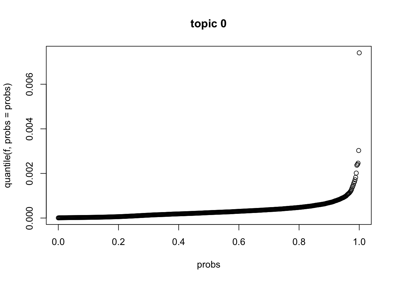
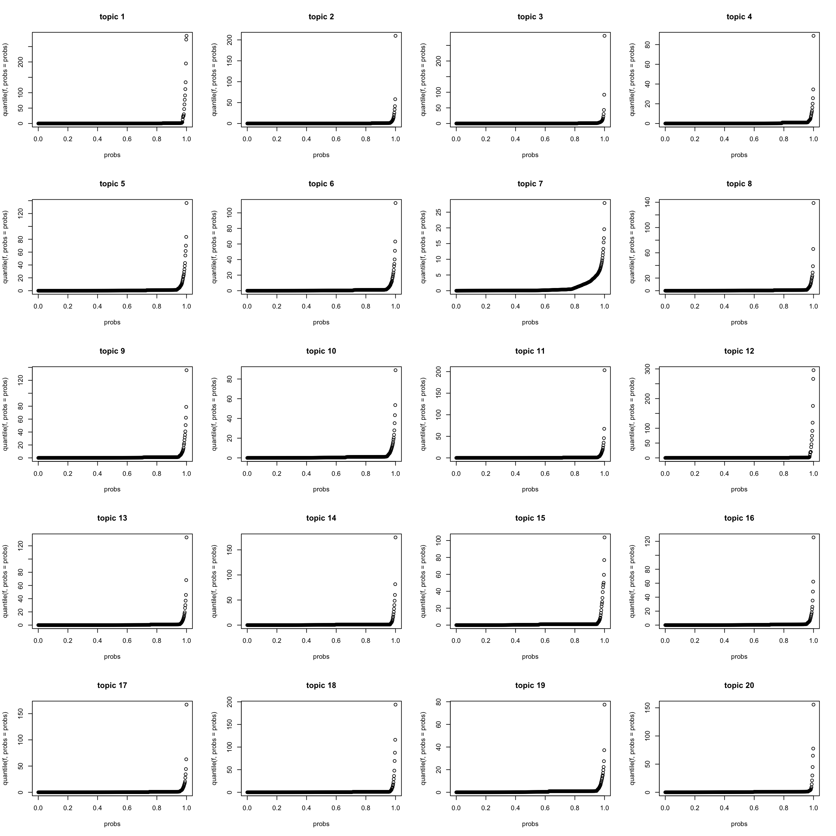
quantile of \(f_{Jk} (k > 0)\) (ebpmf_bg)
K = length(model$qg$gls)
par(mfrow = c(5,4))
for(k in 1:K){
  f = model$qg$qfs_mean[,k]
  probs = seq(0, 1, 0.002)
  plot(probs, quantile(f, probs = probs), main = sprintf("topic %d",k))
}
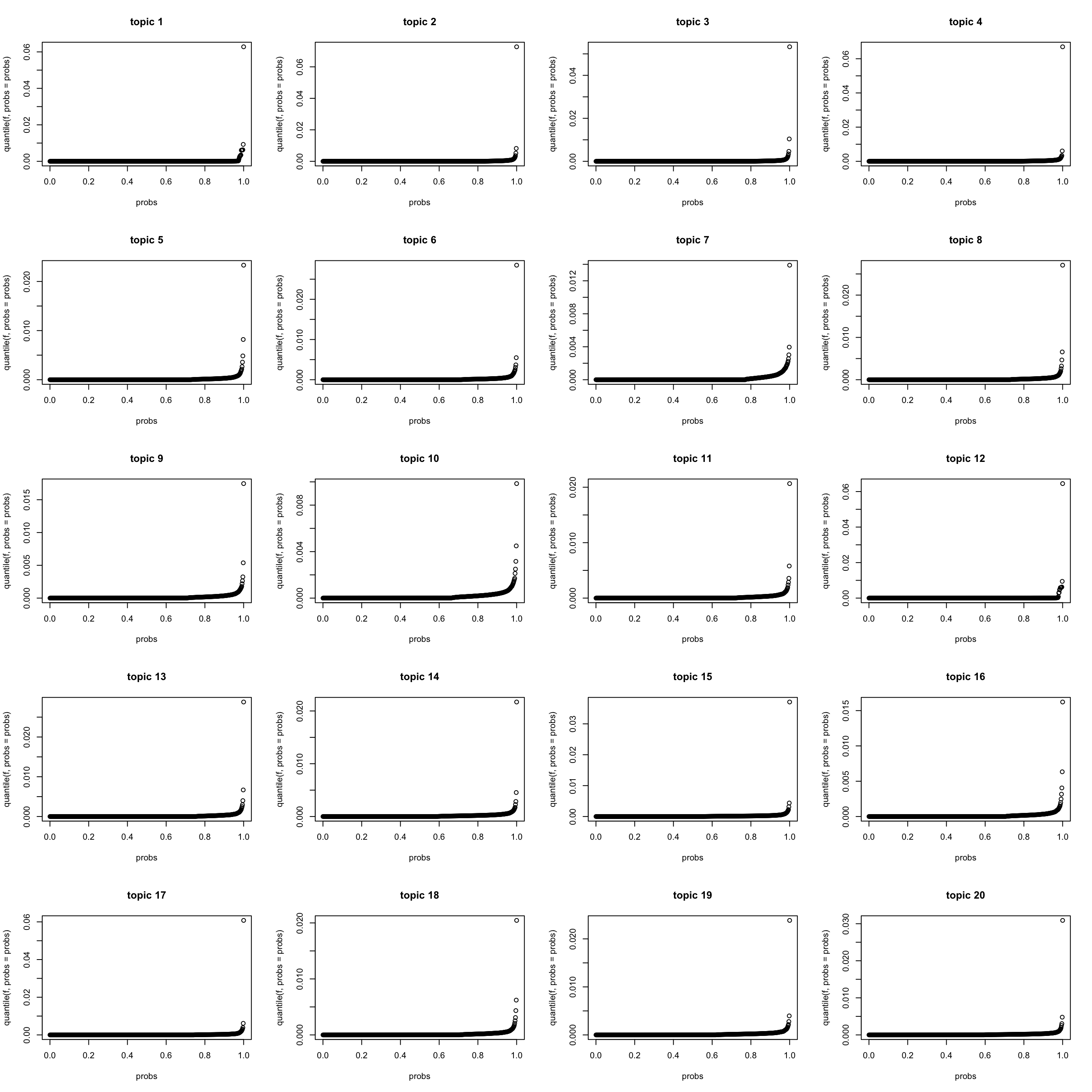
quantile of \(f_{J0} f_{Jk}\) (ebpmf_bg) (scaled to multinom)
lf = poisson2multinom(F = model$f0 * model$qg$qfs_mean,
                 L = model$l0 * model$qg$qls_mean)

K = length(model$qg$gls)
par(mfrow = c(5,4))
for(k in 1:K){
  f = lf$F[,k]
  probs = seq(0, 1, 0.002)
  plot(probs, quantile(f, probs = probs), main = sprintf("topic %d",k))
}
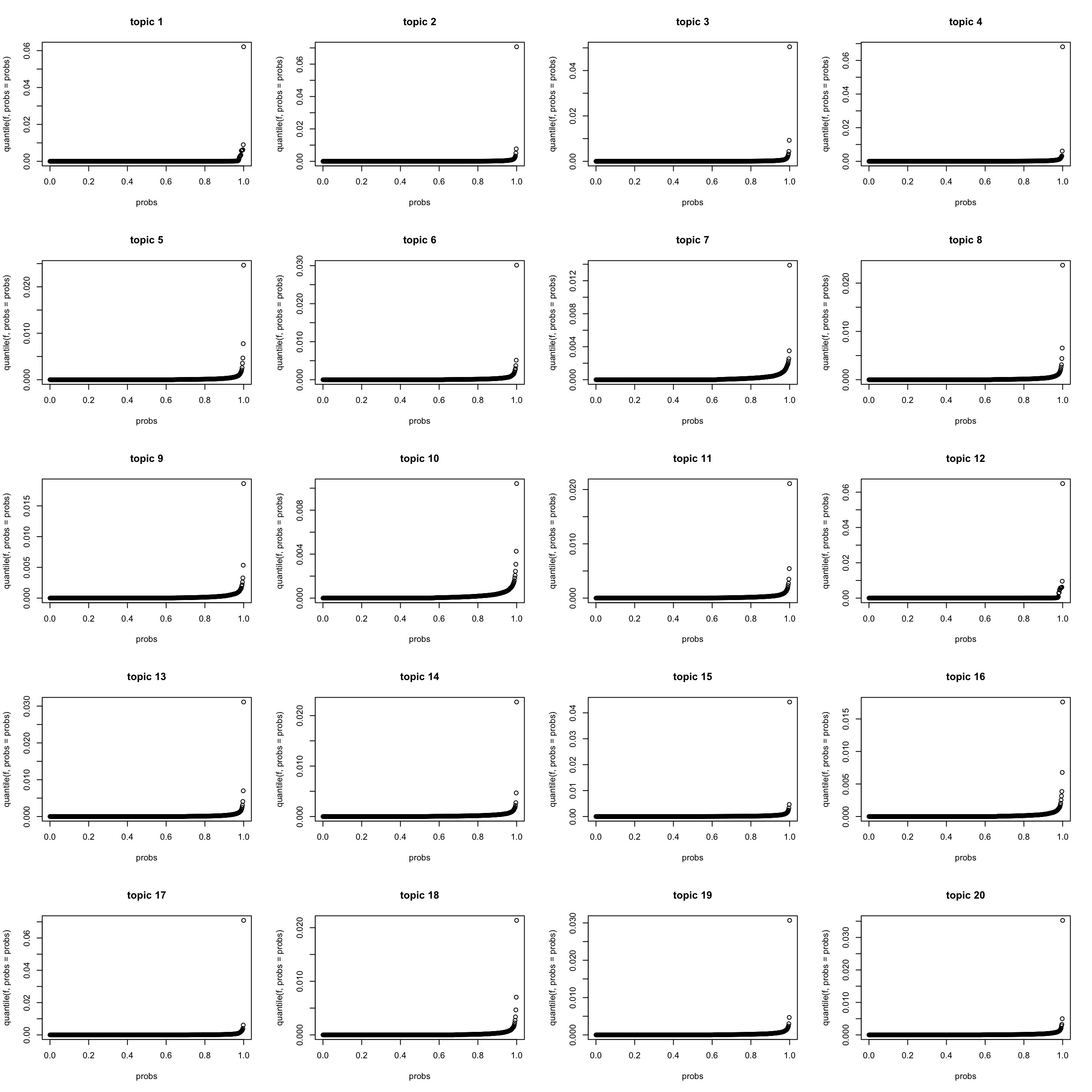
quantile of \(f_{Jk}\) (PMF) (scaled to multinom)
lf_pmf = poisson2multinom(F = model_pmf$F, L = model_pmf$L)
par(mfrow = c(5,4))
for(k in 1:K){
  f = lf_pmf$F[,k]
  probs = seq(0, 1, 0.002)
  plot(probs, quantile(f, probs = probs), main = sprintf("topic %d",k))
}
look at \(s_k\) (ebpmf_bg)
\(s_k := \sum_i l_i0 \bar{l}_{ik}\). I make \(\sum_j f_{j0} = 1\) for interpretability.
d = sum(model$f0)
s_k = colSums(d * model$l0 * model$qg$qls_mean)
names(s_k) <- paste("Topic", 1:K, sep = "")
step = 5
for(i in 1:round(K/step)){
  print(round(s_k[((i-1)*step + 1):(i*step)]))
}
Topic1 Topic2 Topic3 Topic4 Topic5
6459 32515 19832 48767 26860
Topic6 Topic7 Topic8 Topic9 Topic10
23802 20122 21157 22346 24018
Topic11 Topic12 Topic13 Topic14 Topic15
36992 7804 32226 33707 41961
Topic16 Topic17 Topic18 Topic19 Topic20
24284 31774 25470 41837 31661 look at top words for topics
show_topic <- function(k, other_var){
  K = ncol(F)
  n_top_word = other_var$n_top_word
  F = other_var$F
  word_idx = order(F[,k], decreasing = TRUE)[1:n_top_word]
  F_sub = F[word_idx,]
  rownames(F_sub) = dict[word_idx]
  colnames(F_sub) = paste("Topic", 1:K, sep = "")
  pheatmap(F_sub,
           cluster_rows=FALSE, cluster_cols=FALSE,
           silent = TRUE,
           main = sprintf("topic %d", k))[[4]]
}
top words in \(\bar{f}_{Jk}\) (ebpmf_bg)
K_sub = 1:K
p = length(model$l0)
n_top_word = round(0.002 * p)
F = model$qg$qfs_mean[, K_sub]
other_var = list(n_top_word = n_top_word,F = F)
gs = lapply(K_sub, FUN = show_topic, other_var = other_var)
grid.arrange(grobs = gs, ncol = 4)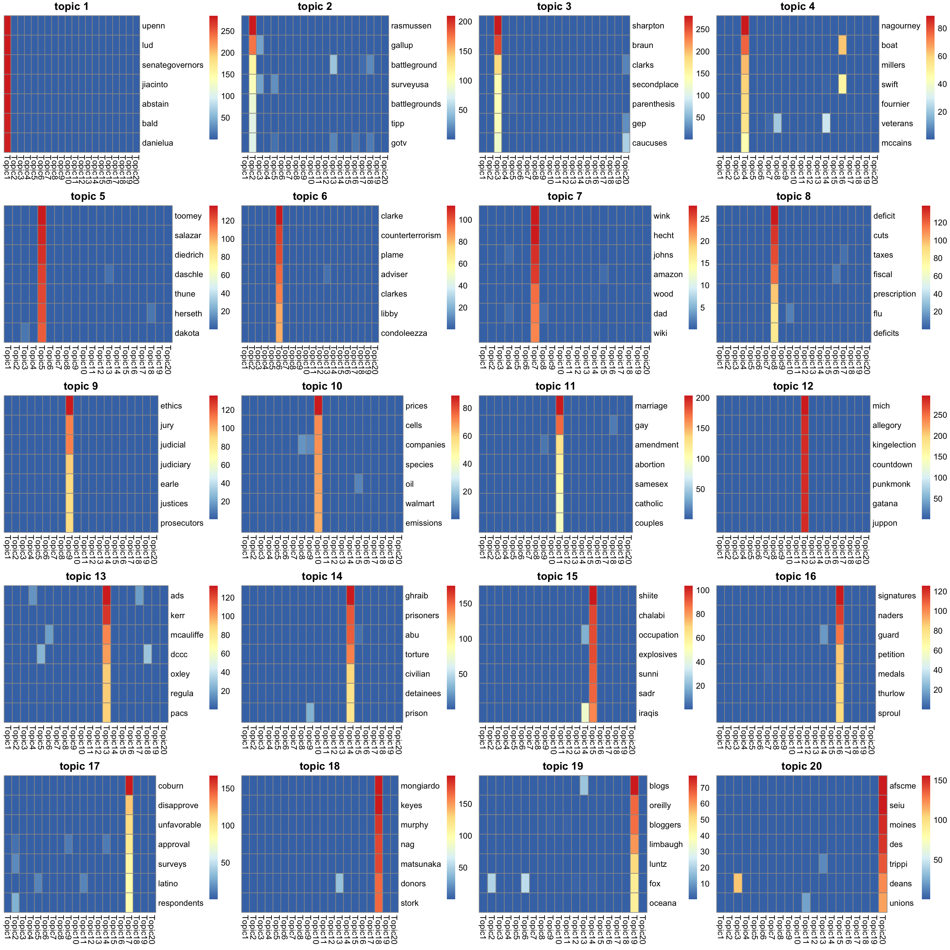
top words in \(f_{J0}\bar{f}_{Jk}\) (ebpmf_bg) (scaled to multinom).
F = lf$F[, K_sub]
other_var = list(n_top_word = n_top_word,F = F)
gs = lapply(K_sub, FUN = show_topic, other_var = other_var)
grid.arrange(grobs = gs, ncol = 4)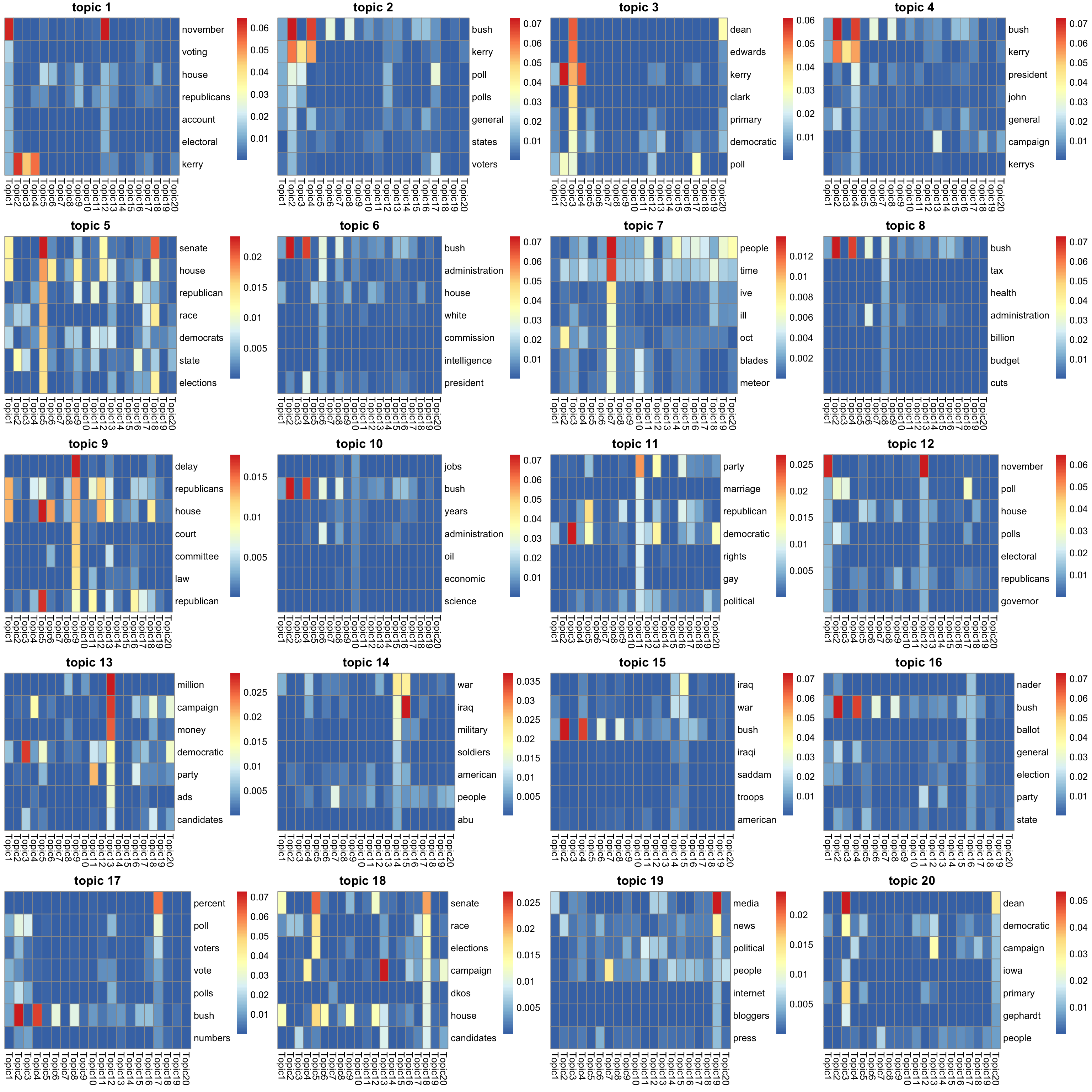
top words in \(f_{jk}\) (PMF) (scaled to multinom).
F = lf_pmf$F[, K_sub]

other_var = list(n_top_word = n_top_word,F = F)
gs = lapply(K_sub, FUN = show_topic, other_var = other_var)
grid.arrange(grobs = gs, ncol = 4)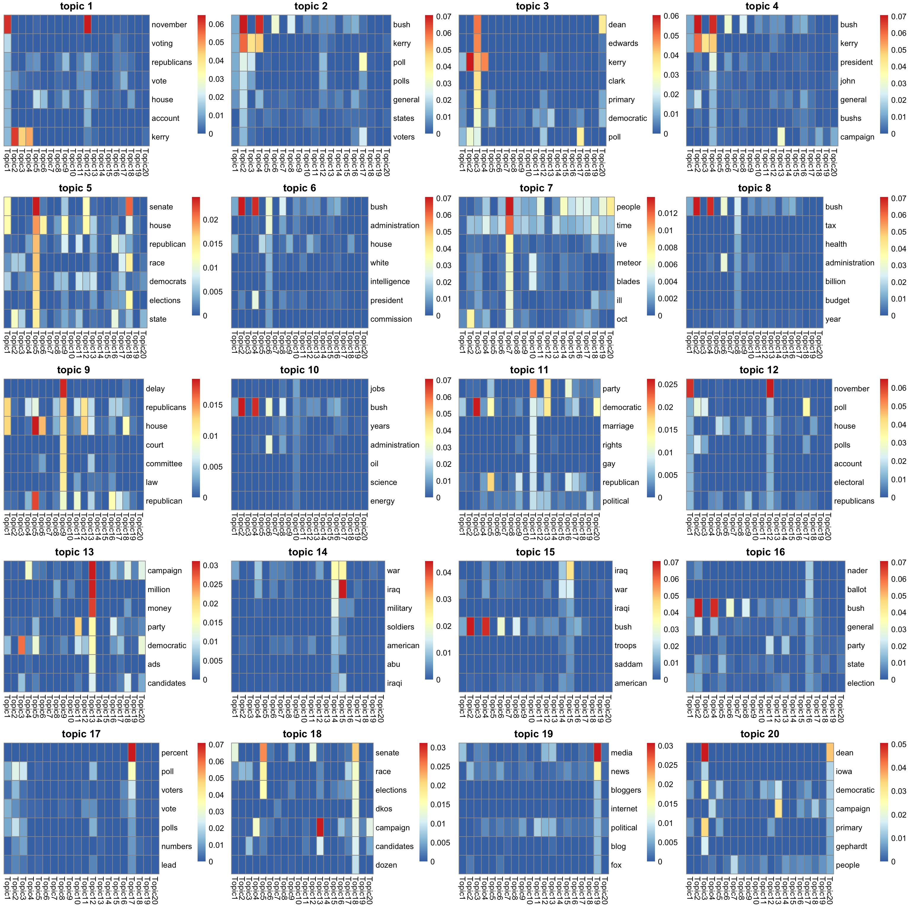
sessionInfo()R version 3.5.1 (2018-07-02)
Platform: x86_64-apple-darwin15.6.0 (64-bit)
Running under: macOS 10.14
Matrix products: default
BLAS: /Library/Frameworks/R.framework/Versions/3.5/Resources/lib/libRblas.0.dylib
LAPACK: /Library/Frameworks/R.framework/Versions/3.5/Resources/lib/libRlapack.dylib
locale:
[1] en_US.UTF-8/en_US.UTF-8/en_US.UTF-8/C/en_US.UTF-8/en_US.UTF-8
attached base packages:
[1] stats graphics grDevices utils datasets methods base
other attached packages:
[1] gridExtra_2.3 pheatmap_1.0.12
loaded via a namespace (and not attached):
[1] Rcpp_1.0.2 knitr_1.28 whisker_0.3-2 magrittr_1.5
[5] workflowr_1.6.2 munsell_0.5.0 colorspace_1.4-1 R6_2.4.0
[9] stringr_1.4.0 tools_3.5.1 grid_3.5.1 gtable_0.3.0
[13] xfun_0.8 git2r_0.26.1 htmltools_0.3.6 yaml_2.2.0
[17] digest_0.6.22 rprojroot_1.3-2 RColorBrewer_1.1-2 later_0.8.0
[21] promises_1.0.1 fs_1.3.1 glue_1.3.1 evaluate_0.14
[25] rmarkdown_2.1 stringi_1.4.3 compiler_3.5.1 scales_1.0.0
[29] backports_1.1.5 httpuv_1.5.1