kos_K100_ebpmf.alpha_v0.3.9
zihao12
2020-05-11
Last updated: 2020-05-16
Checks: 7 0
Knit directory: ebpmf_data_analysis/
This reproducible R Markdown analysis was created with workflowr (version 1.6.2). The Checks tab describes the reproducibility checks that were applied when the results were created. The Past versions tab lists the development history.
Great! Since the R Markdown file has been committed to the Git repository, you know the exact version of the code that produced these results.
Great job! The global environment was empty. Objects defined in the global environment can affect the analysis in your R Markdown file in unknown ways. For reproduciblity it’s best to always run the code in an empty environment.
The command set.seed(20200511) was run prior to running the code in the R Markdown file. Setting a seed ensures that any results that rely on randomness, e.g. subsampling or permutations, are reproducible.
Great job! Recording the operating system, R version, and package versions is critical for reproducibility.
Nice! There were no cached chunks for this analysis, so you can be confident that you successfully produced the results during this run.
Great job! Using relative paths to the files within your workflowr project makes it easier to run your code on other machines.
Great! You are using Git for version control. Tracking code development and connecting the code version to the results is critical for reproducibility.
The results in this page were generated with repository version 20a60fd. See the Past versions tab to see a history of the changes made to the R Markdown and HTML files.
Note that you need to be careful to ensure that all relevant files for the analysis have been committed to Git prior to generating the results (you can use wflow_publish or wflow_git_commit). workflowr only checks the R Markdown file, but you know if there are other scripts or data files that it depends on. Below is the status of the Git repository when the results were generated:
Ignored files:
    Ignored:    .Rhistory
    Ignored:    .Rproj.user/
    Ignored:    analysis/ebpmf_bg_tutorial_cache/

Untracked files:
    Untracked:  code/.util.R.swp
Note that any generated files, e.g. HTML, png, CSS, etc., are not included in this status report because it is ok for generated content to have uncommitted changes.
These are the previous versions of the repository in which changes were made to the R Markdown (analysis/kos_K100_ebpmf.alpha_v0.3.9.Rmd) and HTML (docs/kos_K100_ebpmf.alpha_v0.3.9.html) files. If you’ve configured a remote Git repository (see ?wflow_git_remote), click on the hyperlinks in the table below to view the files as they were in that past version.
| File | Version | Author | Date | Message |
|---|---|---|---|---|
| Rmd | 20a60fd | zihao12 | 2020-05-16 | update analysis for results in v0.3.9 |
| html | 7928026 | zihao12 | 2020-05-16 | Build site. |
| Rmd | 3e38a38 | zihao12 | 2020-05-16 | analysis for results in v0.3.9 |
Introduction
- I apply
ebpmf.alpha(version 0.3.9) to KOS dataset. I use \(K = 100\). The data has \(n = 3430,p = 6906\) and sparsity around \(98\) percent.
- Besides, I also apply to
PMF(lee’s, but I implemented a version for sparse data) to the same dataset with the same initialization. In each iteration,ebpmf_bgdoes two things: MLE for prior and updates posterior. The second part has almost the same computation as inPMF.
model
\[\begin{align} & X_{ij} = \sum_k Z_{ijk}\\ & Z_{ijk} \sim Pois(l_{i0} f_{j0} l_{ik} f_{jk})\\ & l_{ik} \sim g_{L, k}(.), f_{jk} \sim g_{F, k}(.) \end{align}\]For details see ebpmf_bg
prior options
I use gamma mixture \(\sum_l \pi_{l} Ga(1/\phi_l, 1/\phi_l)\) as prior for both \(L, F\). Note that each grid component has \(E = 1, Var = \phi_L\)
initialization
I initialized with 50 runs of NNLM::nnmf (scd). Then I used medians of each row of \(L, F\) as \(l_{i0}, f_{j0}\), and \(l_{ik} = l^0_{ik}/l_{i0}, f_{jk} = f^0_{jk}/f_{j0}\).
library(pheatmap)Warning: package 'pheatmap' was built under R version 3.5.2library(gridExtra)
source("code/misc.R")
output_dir = "output/uci_BoW/v0.3.9/"
data_dir = "data/uci_BoW/"
model_name = "kos_ebpmf_bg_initLF50_K100_maxiter1000.Rds"
model_pmf_name = "kos_pmf_initLF50_K100_maxiter1000.Rds"
dict_name = "vocab.kos.txt"
model = readRDS(sprintf("%s/%s", output_dir, model_name))
model_pmf = readRDS(sprintf("%s/%s", output_dir, model_pmf_name))
dict = read.csv(sprintf("%s/%s", data_dir, dict_name), header = FALSE)[,1]
dict = as.vector(dict)
K = ncol(model_pmf$L)
L_pmf = model_pmf$L; F_pmf = model_pmf$F
L_bg = model$l0 * model$qg$qls_mean; F_bg = model$f0 * model$qg$qfs_mean
lf = poisson2multinom(L=L_bg,F=F_bg)
lf_pmf = poisson2multinom(L = L_pmf,F = F_pmf)ELBO and runtime
plot(model$ELBO, xlab = "niter", ylab = "elbo")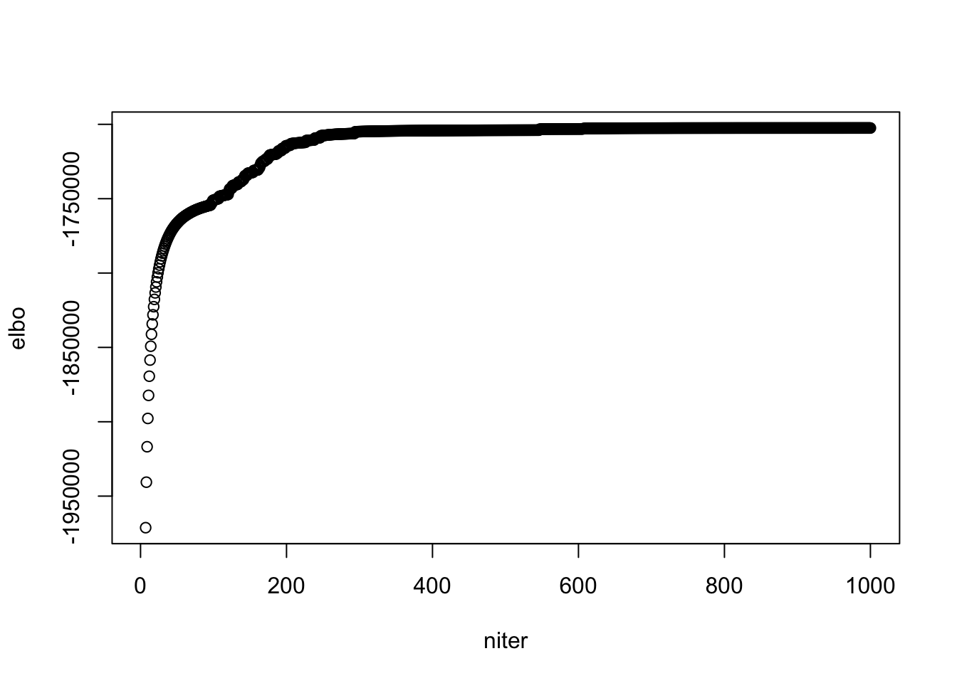
| Version | Author | Date |
|---|---|---|
| 7928026 | zihao12 | 2020-05-16 |
## see when it "converges"
plot(model$ELBO[1:400], xlab = "niter", ylab = "elbo")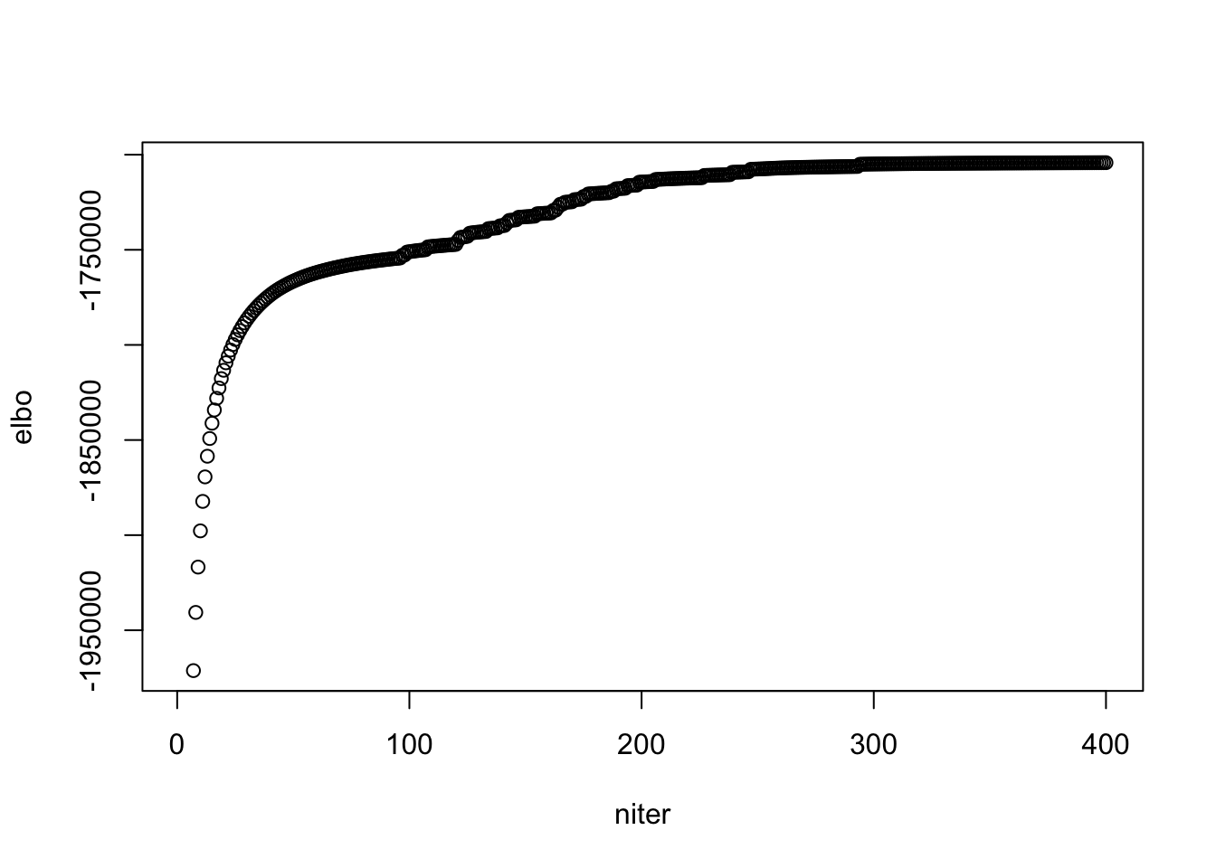
| Version | Author | Date |
|---|---|---|
| 7928026 | zihao12 | 2020-05-16 |
## ebpmf_bg runtime per iteration
model$runtime/length(model$ELBO)
user system elapsed
50.314172 0.136145 50.470211 ## pmf runtime per iteration
model_pmf$runtime/length(model_pmf$log_liks) user system elapsed
23.371322 0.057601 23.437102 look at priors in ebpmf_bg
look at \(s_k\) (ebpmf_bg)
\(s_k := \sum_i l_i0 \bar{l}_{ik}\). I make \(\sum_j f_{j0} = 1\) for interpretability.
d = sum(model$f0)
s_k = colSums(d * model$l0 * model$qg$qls_mean)
names(s_k) <- paste("Topic", 1:K, sep = "")
step = 5
for(i in 1:round(K/step)){
  print(round(s_k[((i-1)*step + 1):(i*step)]))
}
Topic1 Topic2 Topic3 Topic4 Topic5
6100 7463 2527 9813 9611
Topic6 Topic7 Topic8 Topic9 Topic10
2451 5700 11695 7501 5056
Topic11 Topic12 Topic13 Topic14 Topic15
5547 4801 7764 9970 4393
Topic16 Topic17 Topic18 Topic19 Topic20
6855 11303 10004 4446 5743
Topic21 Topic22 Topic23 Topic24 Topic25
6862 2628 7187 7728 8059
Topic26 Topic27 Topic28 Topic29 Topic30
14796 11319 8344 8342 5926
Topic31 Topic32 Topic33 Topic34 Topic35
7371 5690 9397 7500 7162
Topic36 Topic37 Topic38 Topic39 Topic40
7983 6760 5926 4726 6605
Topic41 Topic42 Topic43 Topic44 Topic45
2866 6867 8744 4141 6490
Topic46 Topic47 Topic48 Topic49 Topic50
6272 6405 7473 5720 4669
Topic51 Topic52 Topic53 Topic54 Topic55
6904 6627 6137 8954 5042
Topic56 Topic57 Topic58 Topic59 Topic60
6803 9932 5795 5194 4467
Topic61 Topic62 Topic63 Topic64 Topic65
6985 6906 7221 5321 5497
Topic66 Topic67 Topic68 Topic69 Topic70
7086 6926 8036 6334 4695
Topic71 Topic72 Topic73 Topic74 Topic75
12059 3829 7234 13910 5799
Topic76 Topic77 Topic78 Topic79 Topic80
4038 11648 6461 10701 9003
Topic81 Topic82 Topic83 Topic84 Topic85
11363 13916 5486 5528 7190
Topic86 Topic87 Topic88 Topic89 Topic90
9447 7110 7491 3969 5587
Topic91 Topic92 Topic93 Topic94 Topic95
9672 9673 6689 8947 6647
Topic96 Topic97 Topic98 Topic99 Topic100
5256 14561 6790 7292 6443 look at top words for topics
show_topic <- function(k, other_var){
K = ncol(F)
n_top_word = other_var$n_top_word
F = other_var$F
word_idx = order(F[,k], decreasing = TRUE)[1:n_top_word]
F_sub = F[word_idx,]
rownames(F_sub) = dict[word_idx]
#colnames(F_sub) = paste("Topic", 1:K, sep = "")
colnames(F_sub) = NULL
pheatmap(F_sub,
cluster_rows=FALSE, cluster_cols=FALSE,
silent = TRUE,
main = sprintf("topic %d", k))[[4]]
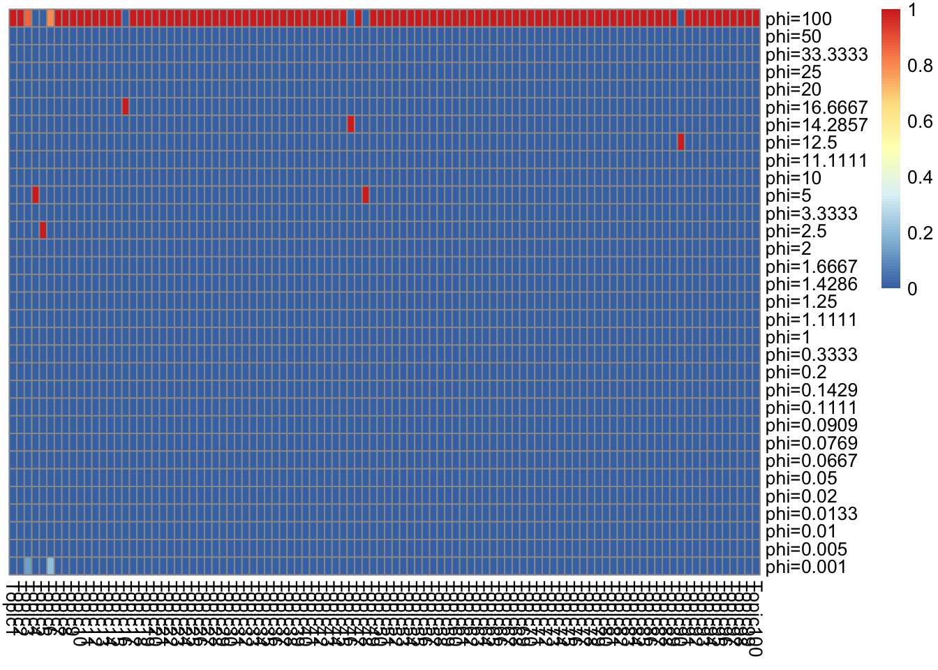
}top words in \(\bar{f}_{Jk}\) (ebpmf_bg)
K_sub = 1:K
p = length(model$l0)
n_top_word = round(0.002 * p)
F = model$qg$qfs_mean[, K_sub]
other_var = list(n_top_word = n_top_word,F = F)
gs = lapply(K_sub, FUN = show_topic, other_var = other_var)
grid.arrange(grobs = gs, ncol = 4)
| Version | Author | Date |
|---|---|---|
| 7928026 | zihao12 | 2020-05-16 |
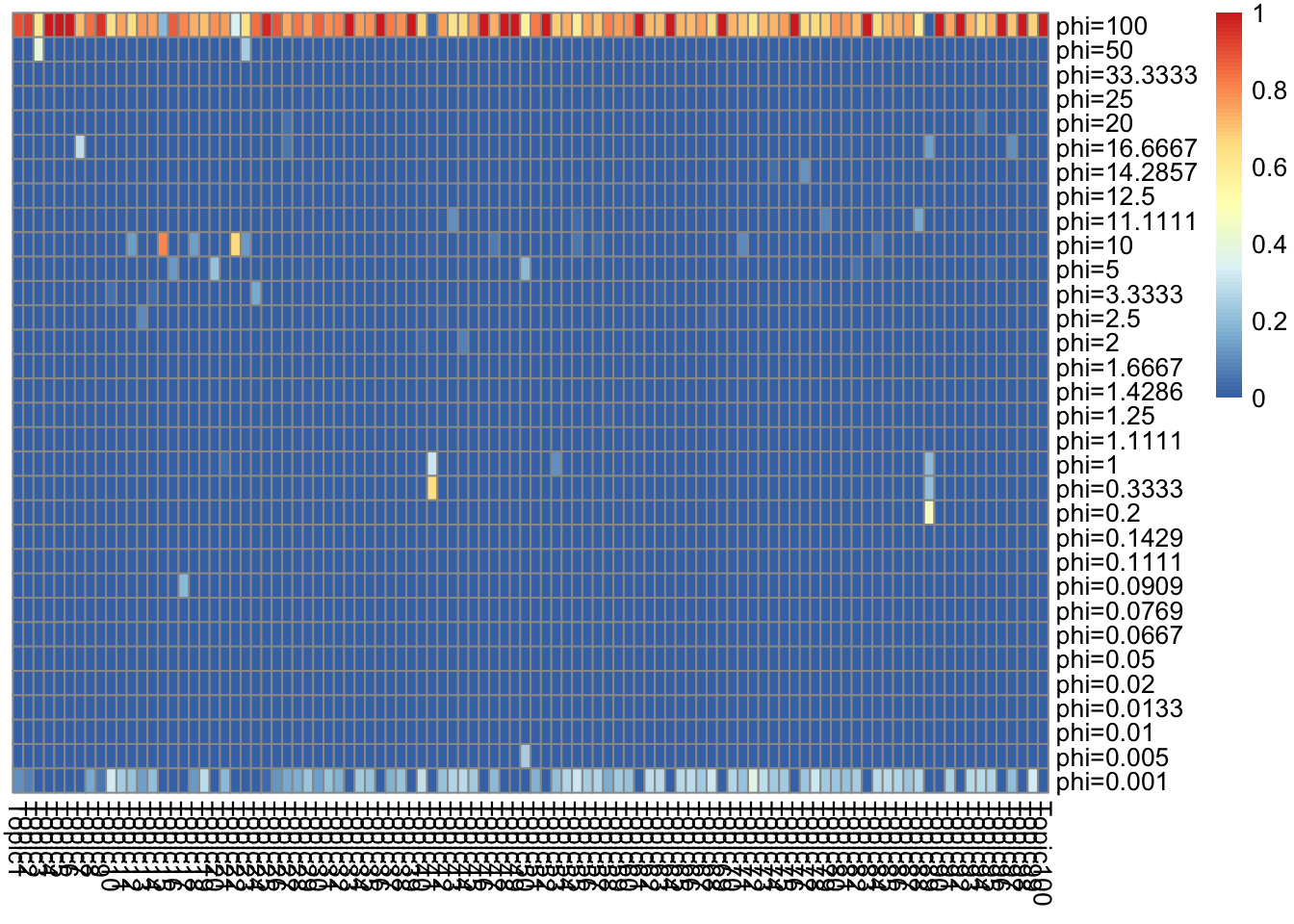
top words in \(f_{J0}\bar{f}_{Jk}\) (ebpmf_bg) (scaled to multinom).
F = lf$F[, K_sub]
other_var = list(n_top_word = n_top_word,F = F)
gs = lapply(K_sub, FUN = show_topic, other_var = other_var)
grid.arrange(grobs = gs, ncol = 4)
| Version | Author | Date |
|---|---|---|
| 7928026 | zihao12 | 2020-05-16 |
top words in \(f_{jk}\) (PMF) (scaled to multinom).
F = lf_pmf$F[, K_sub]

other_var = list(n_top_word = n_top_word,F = F)
gs = lapply(K_sub, FUN = show_topic, other_var = other_var)
grid.arrange(grobs = gs, ncol = 4)
Compare \(L, F\) (in the context of PMF model)
## scale L, F so that colSums(F) = 1
L_pmf = L_pmf %*% diag(colSums(F_pmf))
F_pmf = F_pmf %*% diag(1/colSums(F_pmf))

L_bg = L_bg %*% diag(colSums(F_bg))
F_bg = F_bg %*% diag(1/colSums(F_bg))
\(L\)
par(mfrow = c(25,4))
for(k in 1:K){
  plot(L_pmf[,k], L_bg[,k], pch = 18,
       xlab = "pmf", ylab = "bg", main = sprintf("loading %d", k))
  abline(0,1,lwd=1,col="blue")
}
| Version | Author | Date |
|---|---|---|
| 7928026 | zihao12 | 2020-05-16 |
\(F\)
par(mfrow = c(25,4))
for(k in 1:K){
  plot(F_pmf[,k], F_bg[,k], pch = 18,
       xlab = "pmf", ylab = "bg", main = sprintf("factor %d", k))
  abline(0,1,lwd=1,col="blue")
}
| Version | Author | Date |
|---|---|---|
| 7928026 | zihao12 | 2020-05-16 |
sessionInfo()R version 3.5.1 (2018-07-02)
Platform: x86_64-apple-darwin15.6.0 (64-bit)
Running under: macOS 10.14
Matrix products: default
BLAS: /Library/Frameworks/R.framework/Versions/3.5/Resources/lib/libRblas.0.dylib
LAPACK: /Library/Frameworks/R.framework/Versions/3.5/Resources/lib/libRlapack.dylib
locale:
[1] en_US.UTF-8/en_US.UTF-8/en_US.UTF-8/C/en_US.UTF-8/en_US.UTF-8
attached base packages:
[1] stats graphics grDevices utils datasets methods base
other attached packages:
[1] gridExtra_2.3 pheatmap_1.0.12
loaded via a namespace (and not attached):
[1] Rcpp_1.0.2 knitr_1.28 whisker_0.3-2 magrittr_1.5
[5] workflowr_1.6.2 munsell_0.5.0 colorspace_1.4-1 R6_2.4.0
[9] stringr_1.4.0 tools_3.5.1 grid_3.5.1 gtable_0.3.0
[13] xfun_0.8 git2r_0.26.1 htmltools_0.3.6 yaml_2.2.0
[17] digest_0.6.22 rprojroot_1.3-2 RColorBrewer_1.1-2 later_0.8.0
[21] promises_1.0.1 fs_1.3.1 glue_1.3.1 evaluate_0.14
[25] rmarkdown_2.1 stringi_1.4.3 compiler_3.5.1 scales_1.0.0
[29] backports_1.1.5 httpuv_1.5.1