applications_kos
zihao12
2020-04-29
Last updated: 2020-04-30
Checks: 7 0
Knit directory: ebpmf_demo/
This reproducible R Markdown analysis was created with workflowr (version 1.5.0). The Checks tab describes the reproducibility checks that were applied when the results were created. The Past versions tab lists the development history.
Great! Since the R Markdown file has been committed to the Git repository, you know the exact version of the code that produced these results.
Great job! The global environment was empty. Objects defined in the global environment can affect the analysis in your R Markdown file in unknown ways. For reproduciblity it’s best to always run the code in an empty environment.
The command set.seed(20190923) was run prior to running the code in the R Markdown file. Setting a seed ensures that any results that rely on randomness, e.g. subsampling or permutations, are reproducible.
Great job! Recording the operating system, R version, and package versions is critical for reproducibility.
Nice! There were no cached chunks for this analysis, so you can be confident that you successfully produced the results during this run.
Great job! Using relative paths to the files within your workflowr project makes it easier to run your code on other machines.
Great! You are using Git for version control. Tracking code development and connecting the code version to the results is critical for reproducibility. The version displayed above was the version of the Git repository at the time these results were generated.
Note that you need to be careful to ensure that all relevant files for the analysis have been committed to Git prior to generating the results (you can use wflow_publish or wflow_git_commit). workflowr only checks the R Markdown file, but you know if there are other scripts or data files that it depends on. Below is the status of the Git repository when the results were generated:
Ignored files:
    Ignored:    .RData
    Ignored:    .Rhistory
    Ignored:    .Rproj.user/
    Ignored:    analysis/anchor_word_model_swimmer_cache/
    Ignored:    analysis/compare_GH_cache/
    Ignored:    analysis/compare_speeds_ebpmf_cache/
    Ignored:    analysis/ebpm_two_gamma_debug2_cache/
    Ignored:    analysis/experiment_ebpm_bg2_cache/
    Ignored:    analysis/experiment_ebpm_bg3_cache/
    Ignored:    analysis/experiment_ebpm_bg4_cache/
    Ignored:    analysis/experiment_ebpm_bg5_cache/
    Ignored:    analysis/experiment_ebpm_bg_cache/
    Ignored:    analysis/experiment_ebpm_gammamix2_cache/
    Ignored:    analysis/experiment_ebpm_gammamix3_cache/
    Ignored:    analysis/experiment_ebpm_gammamix_cache/
    Ignored:    analysis/experiment_nb_means3_cache/
    Ignored:    analysis/fit_cytokines_data2_cache/
    Ignored:    analysis/fit_cytokines_data_cache/
    Ignored:    analysis/investigate_gamma_poisson_cache/
    Ignored:    analysis/nmf_anchor_word3_cache/
    Ignored:    analysis/nmf_anchor_word4_cache/
    Ignored:    analysis/nmf_sparse10_cache/
    Ignored:    analysis/nmf_sparse11_cache/
    Ignored:    analysis/nmf_sparse8_cache/
    Ignored:    analysis/nmf_sparse9_cache/
    Ignored:    analysis/test_ebpmf_two_gamma_fast_cache/

Untracked files:
    Untracked:  Rplot.png
    Untracked:  Untitled.Rmd
    Untracked:  Untitled.html
    Untracked:  analysis/.ipynb_checkpoints/
    Untracked:  analysis/Experiment_ebpmf_simple.Rmd
    Untracked:  analysis/anchor_word_model1.Rmd
    Untracked:  analysis/anchor_word_model2.Rmd
    Untracked:  analysis/anchor_word_model3.Rmd
    Untracked:  analysis/compare_speeds_ebpmf.Rmd
    Untracked:  analysis/debug_ebpmf_two_gamma.Rmd
    Untracked:  analysis/demo_ebpmf_beta_gamma.Rmd
    Untracked:  analysis/demo_ebpmf_two_gamma2.Rmd
    Untracked:  analysis/demo_ebpmf_two_gamma_cache_old/
    Untracked:  analysis/draft.Rmd
    Untracked:  analysis/ebpm_gamma_mixture_experiment.Rmd
    Untracked:  analysis/ebpm_gh_gamma.Rmd
    Untracked:  analysis/ebpm_two_gamma_test.R
    Untracked:  analysis/ebpm_two_gamma_test.Rmd
    Untracked:  analysis/ebpmf.Rmd
    Untracked:  analysis/ebpmf_demo.Rmd
    Untracked:  analysis/ebpmf_rank1_demo2.Rmd
    Untracked:  analysis/ebpmf_two_gamma_debug.Rmd
    Untracked:  analysis/experiment_ebpm_bg2.Rmd
    Untracked:  analysis/experiment_ebpm_bg5_cache_old/
    Untracked:  analysis/experiment_nb_means2_cache_0/
    Untracked:  analysis/experiment_nb_means3.Rmd
    Untracked:  analysis/experiment_nb_means4.Rmd
    Untracked:  analysis/experiment_nb_means_old.Rmd
    Untracked:  analysis/fit_cytokines_data2.Rmd
    Untracked:  analysis/fit_cytokines_data_old.Rmd
    Untracked:  analysis/investigate_ebpm_s.Rmd
    Untracked:  analysis/investigate_gamma_poisson.Rmd
    Untracked:  analysis/investigate_nmf_sparse.Rmd
    Untracked:  analysis/nmf_anchor_word4.Rmd
    Untracked:  analysis/nmf_sparse11.Rmd
    Untracked:  analysis/nmf_symm.Rmd
    Untracked:  analysis/play_prior.Rmd
    Untracked:  analysis/play_shrinkage_methods.Rmd
    Untracked:  analysis/plot_g.Rmd
    Untracked:  analysis/rebayes_vignette.Rmd
    Untracked:  analysis/simulate_nb_means.Rmd
    Untracked:  analysis/softmax_experiments.ipynb
    Untracked:  analysis/test_ebpmf_two_gamma_fast.Rmd
    Untracked:  analysis/try_CVXR.Rmd
    Untracked:  cache/
    Untracked:  code/anchor-word-recovery/
    Untracked:  data/anchor_word_model1.csv
    Untracked:  data/cytokines_data_bg_model.rds
    Untracked:  data/cytokines_data_fit.RData
    Untracked:  data/cytokines_fit_bg2.Rds
    Untracked:  data/genes_ranked.RDS
    Untracked:  data/nmf_anchor_word3_A.csv
    Untracked:  data/nmf_anchor_word3_W.csv
    Untracked:  data/nmf_anchor_word3_X.csv
    Untracked:  data/nmf_anchor_word4_A.csv
    Untracked:  data/nmf_anchor_word4_W.csv
    Untracked:  data/nmf_sparse8_fit_ebpmf_gm_mle.Rds
    Untracked:  data/nmf_sparse8_fit_ebpmf_gm_mlem.Rds
    Untracked:  data/nmf_sparse_ebpm_tg_slow.Rds
    Untracked:  data/scdata_hvg.RDS
    Untracked:  data/scdata_lvg.RDS
    Untracked:  data/swimmer.mat
    Untracked:  figure/
    Untracked:  script/ebpm_background.R
    Untracked:  script/nb_means_old.R
    Untracked:  script/nmf_sparse_ebpm_old.R
    Untracked:  script/sim_bg_model.R
    Untracked:  script/test_nb_means_cytokines.R
    Untracked:  verbose_log_1571583163.21966.txt
    Untracked:  verbose_log_1571583324.71036.txt
    Untracked:  verbose_log_1571583741.94199.txt
    Untracked:  verbose_log_1571588102.40356.txt

Unstaged changes:
    Modified:   analysis/experiment_ebpm_bg.Rmd
    Modified:   analysis/experiment_ebpm_bg5.Rmd
    Modified:   analysis/experiment_nb_means.Rmd
    Deleted:    analysis/experiment_nb_means_cache/html/__globals
    Deleted:    analysis/experiment_nb_means_cache/html/__objects
    Deleted:    analysis/experiment_nb_means_cache/html/__packages
    Deleted:    analysis/experiment_nb_means_cache/html/unnamed-chunk-3_ac840b1b9f49c0bc24b3f3b2ad41215e.RData
    Deleted:    analysis/experiment_nb_means_cache/html/unnamed-chunk-3_ac840b1b9f49c0bc24b3f3b2ad41215e.rdb
    Deleted:    analysis/experiment_nb_means_cache/html/unnamed-chunk-3_ac840b1b9f49c0bc24b3f3b2ad41215e.rdx
    Modified:   script/test_nb_means.R
    Modified:   script/test_nb_means2.R
Note that any generated files, e.g. HTML, png, CSS, etc., are not included in this status report because it is ok for generated content to have uncommitted changes.
These are the previous versions of the R Markdown and HTML files. If you’ve configured a remote Git repository (see ?wflow_git_remote), click on the hyperlinks in the table below to view them.
| File | Version | Author | Date | Message |
|---|---|---|---|---|
| Rmd | 70b3375 | zihao12 | 2020-04-30 | update applications_kos |
| html | e29a1ee | zihao12 | 2020-04-30 | Build site. |
| Rmd | 5eba64a | zihao12 | 2020-04-30 | applications_kos.Rmd |
Introduction
- I applied Poisson Matrix Factorization to analyze a corpus of Daily Kos Blog dataset.
- The data is downloaded from Bag of Words. I run
NNLM::nnmffor \(1000\) iterations with \(20\) topics, usingscdalgorithm.
- I mainly look at \(f_{jK}\) of the fitted model.
- Note that, I use \(s_k f_{jk}\) in place of \(f_{jk}\) for fear that some small non-zero numbers will be read as 0.
rm(list = ls())
library(Matrix)
Warning: package 'Matrix' was built under R version 3.5.2source("code/misc.R")
set.seed(123)
data_dir = "~/Desktop/data/text"
data_name = "docword.kos.mtx"
model_name = "docword.kos_nnmf_K20_maxiter1000.Rds"
dict_name = "vocab.kos.txt"
Y = readMM(file= sprintf("%s/%s", data_dir, data_name))
Y = as.matrix(Y)
dict = read.csv(sprintf("%s/%s", data_dir, dict_name), header = FALSE)
dict = as.vector(dict[,1])
model = readRDS(sprintf("%s/%s", data_dir, model_name))
L = model$W
F = t(model$H)
## scale F
s_k = colSums(L)
F = t(t(F) * s_k)
dim(Y)[1] 3430 6906dim(L)[1] 3430 20dim(F)[1] 6906 20n = nrow(Y)
p = ncol(Y)
K = ncol(L)
## scale l,f into multinomial model
lf = poisson2multinom(F = F, L = L)look at the meaning of each topic
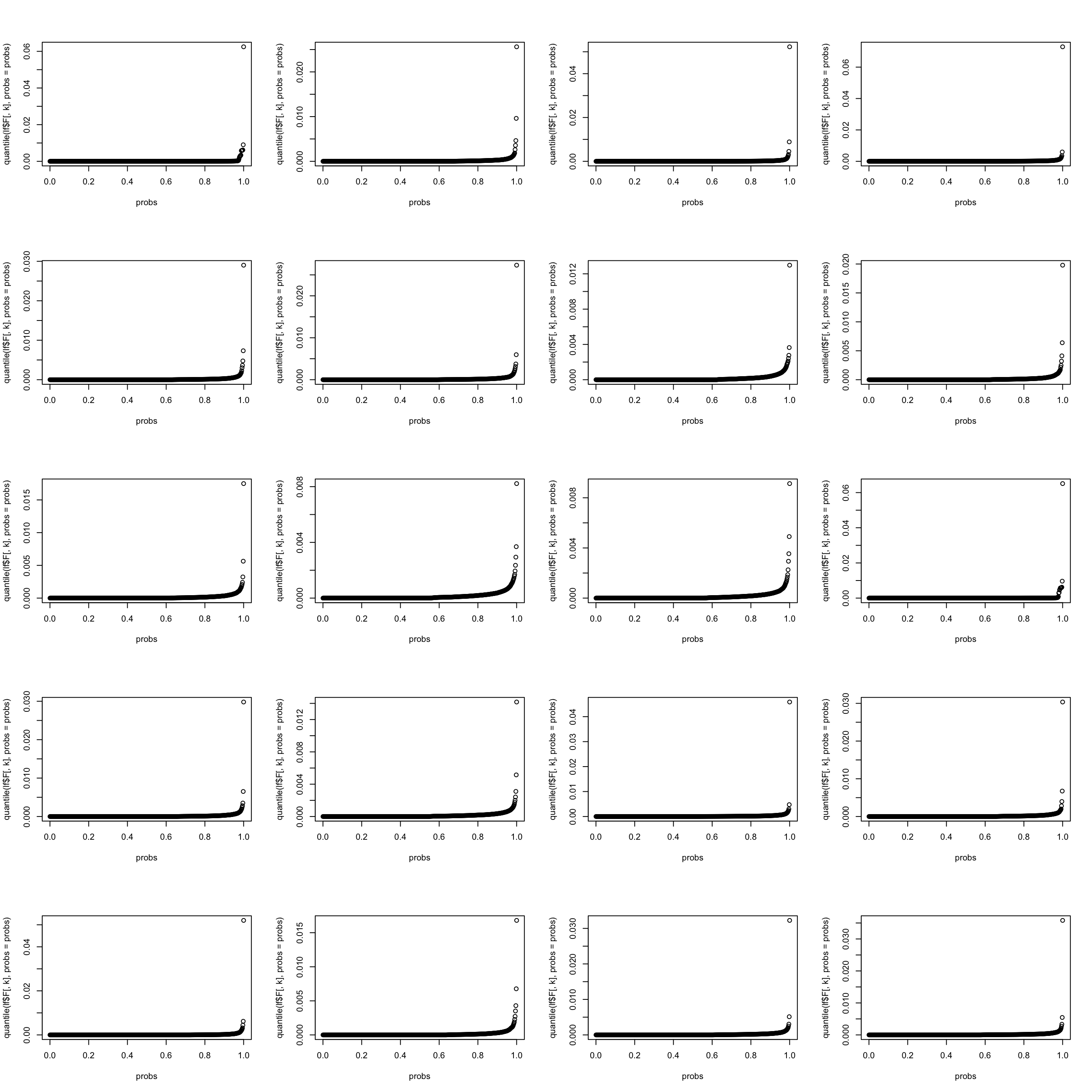
let’s look at the weight distribution in each topic (multinomial model). It seems that the top \(0.002\) words take up most weight.
par(mfrow = c(5,4))
for(k in 1:K){
  probs = seq(0, 1, 0.002)
  #top_words = order(lf$F[,1], decreasing = TRUE)[1:13]
  plot(probs, quantile(lf$F[,k], probs = probs))
}
| Version | Author | Date |
|---|---|---|
| e29a1ee | zihao12 | 2020-04-30 |
Below I show the top \(0.002\) words in each topic (per column)
n_word = round(0.002 * p)
topic_df <- matrix(,nrow = n_word, ncol = K)
for(k in 1:K){
  topic_df[,k] = dict[order(lf$F[,k], decreasing = TRUE)[1:n_word]]
}
colnames(topic_df) <- 1:K
topic_df
1 2 3 4 5
[1,] "november" "states" "dean" "bush" "senate"
[2,] "voting" "state" "edwards" "kerry" "race"
[3,] "kerry" "election" "kerry" "president" "house"
[4,] "account" "nader" "clark" "john" "republican"
[5,] "republicans" "vote" "primary" "general" "elections"
[6,] "house" "party" "democratic" "bushs" "democrats"
[7,] "vote" "ballot" "lieberman" "campaign" "seat"
[8,] "senate" "general" "poll" "cheney" "state"
[9,] "electoral" "florida" "gephardt" "debate" "gop"
[10,] "governor" "voters" "iowa" "kerrys" "democratic"
[11,] "poll" "republican" "kucinich" "george" "carson"
[12,] "polls" "votes" "results" "war" "primary"
[13,] "bush" "ohio" "sharpton" "iraq" "democrat"
[14,] "election" "democratic" "numbers" "speech" "south"
6 7 8 9
[1,] "bush" "time" "bush" "delay"
[2,] "administration" "people" "tax" "republicans"
[3,] "intelligence" "ive" "jobs" "house"
[4,] "house" "ill" "health" "committee"
[5,] "white" "meteor" "economy" "court"
[6,] "president" "blades" "administration" "republican"
[7,] "commission" "oct" "billion" "texas"
[8,] "report" "general" "year" "bill"
[9,] "iraq" "youre" "budget" "senate"
[10,] "terrorism" "dkos" "economic" "democrats"
[11,] "cia" "night" "cuts" "law"
[12,] "security" "live" "million" "federal"
[13,] "officials" "heres" "care" "ethics"
[14,] "weapons" "lot" "job" "investigation"
10 11 12 13 14
[1,] "bush" "rights" "november" "campaign" "war"
[2,] "years" "marriage" "poll" "party" "military"
[3,] "oil" "gay" "house" "million" "iraq"
[4,] "administration" "people" "polls" "money" "abu"
[5,] "energy" "amendment" "electoral" "democratic" "rumsfeld"
[6,] "space" "issue" "governor" "ads" "ghraib"
[7,] "science" "women" "account" "democrats" "american"
[8,] "blades" "political" "republicans" "dnc" "general"
[9,] "meteor" "reagan" "senate" "candidates" "people"
[10,] "research" "party" "trouble" "political" "defense"
[11,] "policy" "american" "ground" "bush" "iraqi"
[12,] "environmental" "conservative" "turnout" "national" "soldiers"
[13,] "cell" "president" "contact" "republicans" "pentagon"
[14,] "gas" "vote" "duderino" "election" "prisoners"
15 16 17 18 19
[1,] "iraq" "bush" "bush" "district" "media"
[2,] "war" "service" "poll" "race" "news"
[3,] "iraqi" "kerry" "kerry" "senate" "bloggers"
[4,] "troops" "military" "percent" "house" "internet"
[5,] "american" "bushs" "polls" "elections" "press"
[6,] "forces" "war" "voters" "candidates" "fox"
[7,] "killed" "national" "polling" "campaign" "book"
[8,] "military" "guard" "results" "races" "conservative"
[9,] "baghdad" "vietnam" "general" "candidate" "blogs"
[10,] "soldiers" "draft" "numbers" "dkos" "radio"
[11,] "saddam" "veterans" "lead" "money" "coverage"
[12,] "bush" "records" "race" "republican" "political"
[13,] "country" "texas" "vote" "obama" "blog"
[14,] "attacks" "duty" "undecided" "dozen" "tom"
20
[1,] "dean"
[2,] "iowa"
[3,] "democratic"
[4,] "campaign"
[5,] "primary"
[6,] "endorsement"
[7,] "howard"
[8,] "gephardt"
[9,] "people"
[10,] "deans"
[11,] "unions"
[12,] "union"
[13,] "candidate"
[14,] "edwards" Let’s look at the structure of \(f_{jk}\).
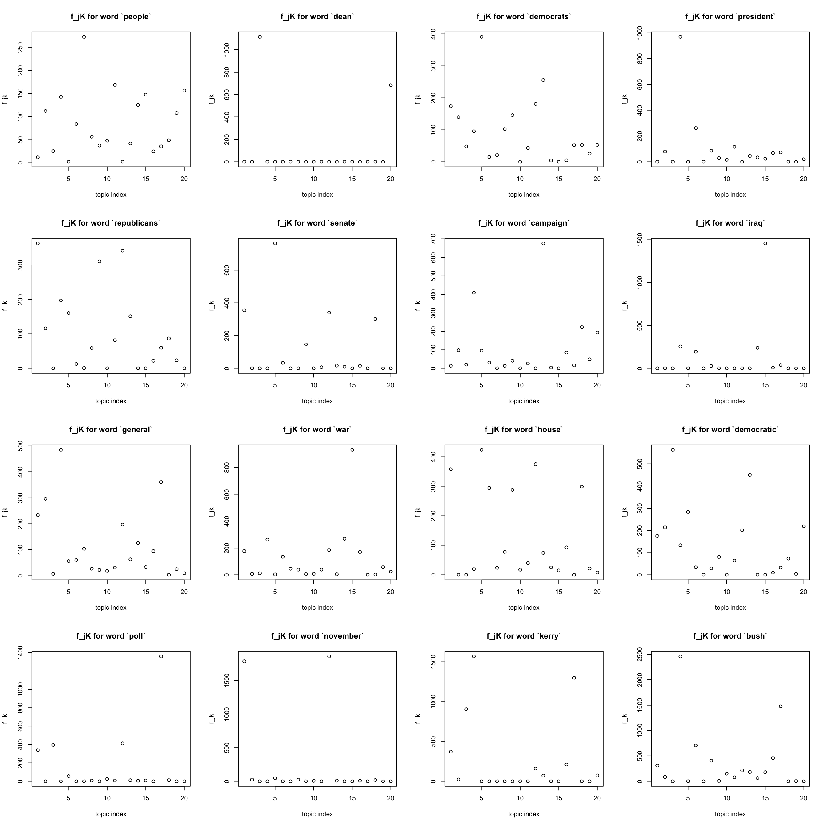
most frequent words
Note that the most frequent words (like “a”, “the”)seem to have been eliminated …
freq_order = order(colSums(Y)) ## increasing order

#idx = sample(x = 1:p, size = 9, replace = FALSE)
idx = freq_order[(p-15):p]
par(mfrow = c(4,4))
for(j in idx){
  plot(F[j,], xlab = "topic index", ylab = "f_jk",
       main = sprintf("f_jK for word `%s`", dict[j]))
}
| Version | Author | Date |
|---|---|---|
| e29a1ee | zihao12 | 2020-04-30 |
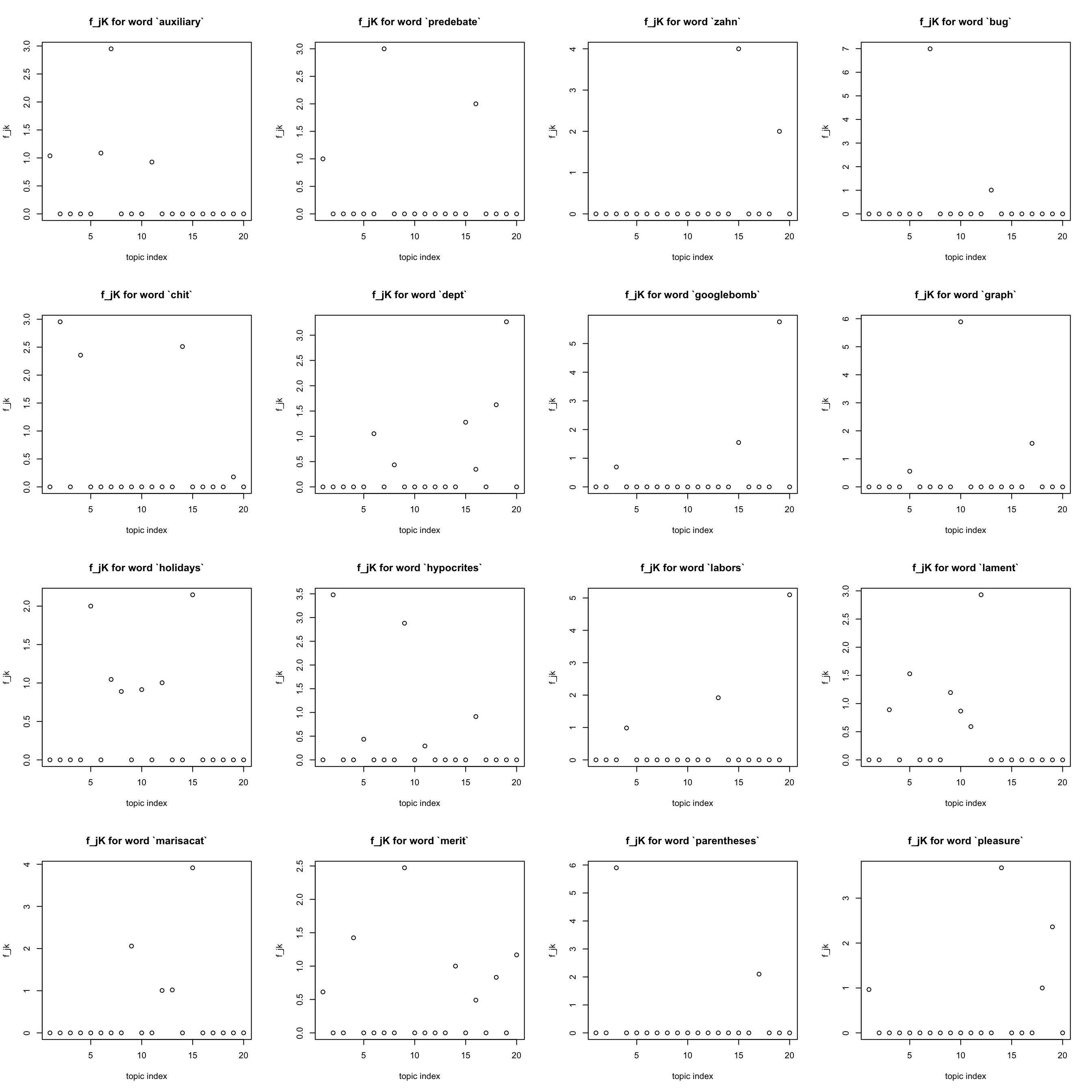
rarest words
Also note that words that occurred less than ten times are also eliminated
idx = freq_order[1:16]
par(mfrow = c(4,4))
for(j in idx){
  plot(F[j,], xlab = "topic index", ylab = "f_jk",
       main = sprintf("f_jK for word `%s`", dict[j]))
}
| Version | Author | Date |
|---|---|---|
| e29a1ee | zihao12 | 2020-04-30 |
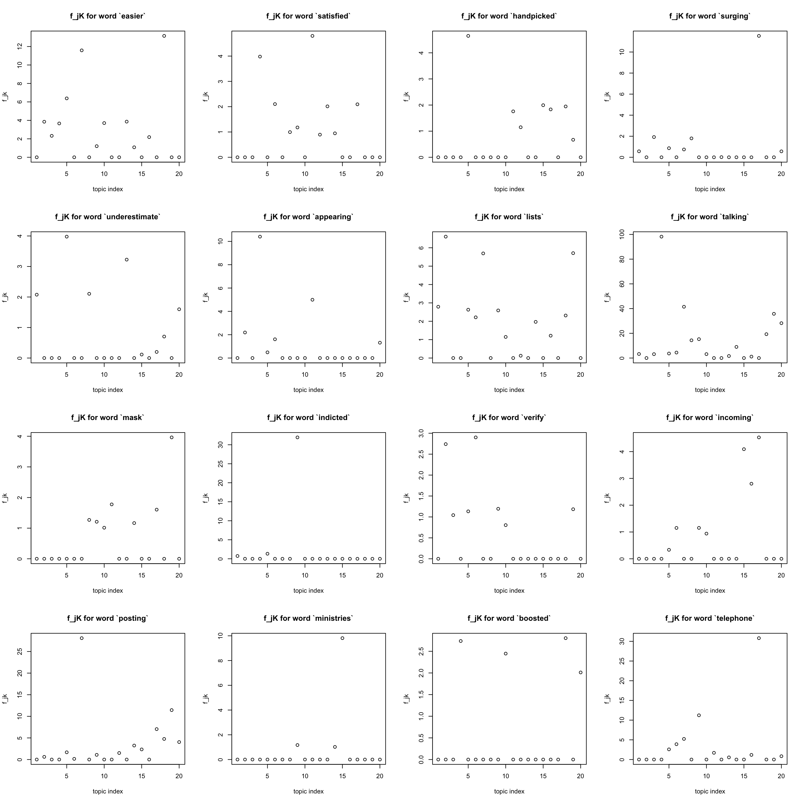
other words
get some words that are neither most often nor rare
idx = sample(x = 1:p, size = 16, replace = FALSE) ## hope it won't coincide with previous choices
par(mfrow = c(4,4))
for(j in idx){
  plot(F[j,], xlab = "topic index", ylab = "f_jk",
       main = sprintf("f_jK for word `%s`", dict[j]))
}
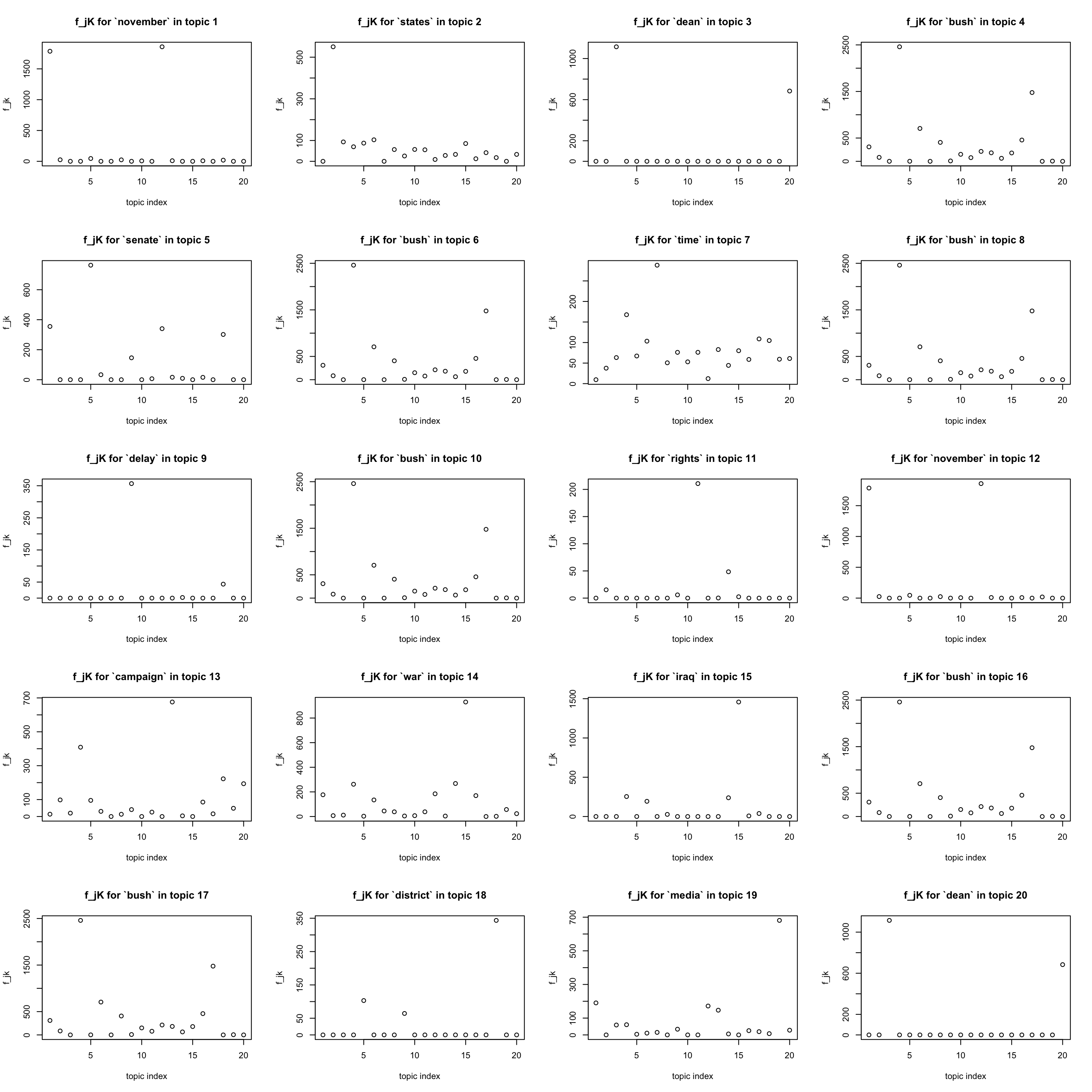
most important words in a topic
par(mfrow = c(5,4))
for(k in 1:K){
  j = which.max(lf$F[,k])
  plot(F[j,], xlab = "topic index", ylab = "f_jk",
       main = sprintf("f_jK for `%s` in topic %d", dict[j], k))
}
sessionInfo()R version 3.5.1 (2018-07-02)
Platform: x86_64-apple-darwin15.6.0 (64-bit)
Running under: macOS 10.14
Matrix products: default
BLAS: /Library/Frameworks/R.framework/Versions/3.5/Resources/lib/libRblas.0.dylib
LAPACK: /Library/Frameworks/R.framework/Versions/3.5/Resources/lib/libRlapack.dylib
locale:
[1] en_US.UTF-8/en_US.UTF-8/en_US.UTF-8/C/en_US.UTF-8/en_US.UTF-8
attached base packages:
[1] stats graphics grDevices utils datasets methods base
other attached packages:
[1] Matrix_1.2-17
loaded via a namespace (and not attached):
[1] workflowr_1.5.0 Rcpp_1.0.2 lattice_0.20-38 rprojroot_1.3-2
[5] digest_0.6.22 later_0.8.0 grid_3.5.1 R6_2.4.0
[9] backports_1.1.5 git2r_0.26.1 magrittr_1.5 evaluate_0.14
[13] stringi_1.4.3 fs_1.3.1 promises_1.0.1 whisker_0.3-2
[17] rmarkdown_2.1 tools_3.5.1 stringr_1.4.0 glue_1.3.1
[21] httpuv_1.5.1 xfun_0.8 yaml_2.2.0 compiler_3.5.1
[25] htmltools_0.3.6 knitr_1.28