ebpm_demo
zihao12
2019-09-23
Last updated: 2019-09-24
Checks: 7 0
Knit directory: ebpmf/
This reproducible R Markdown analysis was created with workflowr (version 1.4.0). The Checks tab describes the reproducibility checks that were applied when the results were created. The Past versions tab lists the development history.
Great! Since the R Markdown file has been committed to the Git repository, you know the exact version of the code that produced these results.
Great job! The global environment was empty. Objects defined in the global environment can affect the analysis in your R Markdown file in unknown ways. For reproduciblity it’s best to always run the code in an empty environment.
The command set.seed(20190923) was run prior to running the code in the R Markdown file. Setting a seed ensures that any results that rely on randomness, e.g. subsampling or permutations, are reproducible.
Great job! Recording the operating system, R version, and package versions is critical for reproducibility.
Nice! There were no cached chunks for this analysis, so you can be confident that you successfully produced the results during this run.
Great job! Using relative paths to the files within your workflowr project makes it easier to run your code on other machines.
Great! You are using Git for version control. Tracking code development and connecting the code version to the results is critical for reproducibility. The version displayed above was the version of the Git repository at the time these results were generated.
Note that you need to be careful to ensure that all relevant files for the analysis have been committed to Git prior to generating the results (you can use wflow_publish or wflow_git_commit). workflowr only checks the R Markdown file, but you know if there are other scripts or data files that it depends on. Below is the status of the Git repository when the results were generated:
Ignored files:
    Ignored:    .Rhistory
    Ignored:    .Rproj.user/

Untracked files:
    Untracked:  analysis/ebpmf_demo.Rmd
Note that any generated files, e.g. HTML, png, CSS, etc., are not included in this status report because it is ok for generated content to have uncommitted changes.
These are the previous versions of the R Markdown and HTML files. If you’ve configured a remote Git repository (see ?wflow_git_remote), click on the hyperlinks in the table below to view them.
| File | Version | Author | Date | Message |
|---|---|---|---|---|
| Rmd | 731df2d | zihao12 | 2019-09-24 | update deno |
| html | aa84714 | zihao12 | 2019-09-24 | Build site. |
| Rmd | c1164b4 | zihao12 | 2019-09-24 | demo ebpm update grid range |
| html | 25f8b5a | zihao12 | 2019-09-24 | Build site. |
| Rmd | a92d9ab | zihao12 | 2019-09-24 | demo ebpm update grid range |
| html | 06d1f33 | zihao12 | 2019-09-24 | Build site. |
| Rmd | 5e5f539 | zihao12 | 2019-09-24 | demo ebpm update |
| html | 9e28fe2 | zihao12 | 2019-09-23 | Build site. |
| Rmd | fdb63ad | zihao12 | 2019-09-23 | demo ebpm |
EBPM problem
see detail in …
library(mixsqp)
library(ggplot2)
Warning: package 'ggplot2' was built under R version 3.5.2library(gtools)
#library(bsts)EBPM-gamma
- For now, I use mixture of exponential as prior family.
- Under the exponential case, we discuss how to select the range of the grid (of \(\mu\)). For convenience we use \(exp(\mu)\) to denote exponential distribution with mean \(\mu\):
The goal is: for each observation, we want to include the range of \(\lambda\) “of interest” (i.e. \(log \ p(x | \lambda)\) is close to that of the MLE, like within \(log(0.1)\)). If \(x = 0\), \(\ell(\lambda) = - \lambda s\), in order to have a good likelihood, we want the model to be able to choose \(\lambda \sim o(\frac{1}{s})\). Therefore, we want the smallest \(\mu\) to be in the order of \(o(\frac{1}{s})\) if there is 0 count.
If \(x > 0\), the MLE would be \(\frac{x}{s}\), and \(\lambda\) too small would have bad likelihood. So we want the biggest \(\mu\) to be of order \(O(max(\frac{x}{s}))\)
compute_L <- function(x, s,a, b){
  M1 = (s^x)/gamma(x + 1)
  M2 = (b^a)/gamma(a)
  ak_add_xi = outer(x,a, "+")
  M3 = gamma(ak_add_xi)/outer(s,b, "+")^ak_add_xi
  out = outer(M1, M2, "*") * M3
  return(out)
}

## generate a geometric sequence: x_n = low*m^{n-1} up to x_n < up
geom_seq <- function(low, up, m){
  N =  ceiling(log(up/low)/log(m)) + 1
  out  = low*m^(seq(1,N, by = 1)-1)
  return(out)
}

select_grid <- function(x, s, m = 2){
  ## mu_grid: mu =  1/b
  x_d_s = x/s
  xprime = x
  xprime[x == 0] = xprime[x == 0] + 1
  xprime_d_s = xprime/s
  #mu_grid = seq(0.1*min(xprime_d_s),2*max(x_d_s), length.out = nv)
  mu_grid_min =  0.1*min(xprime_d_s)
  mu_grid_max = 2*max(x_d_s)
  mu_grid = geom_seq(mu_grid_min, mu_grid_max, m)

  a = rep(1,length(mu_grid))
  b = 1/mu_grid
  return(list(a = a, b  = b))
}

ebpm <- function(x,s,nv = 100, grid = NULL, seed = 123){
  set.seed(seed)
  if(is.null(grid)){grid <- select_grid(x,s,nv)}
  a = grid$a
  b =  grid$b
  L <-  compute_L(x,s,a,b)
  fit <- mixsqp(L, control = list(verbose = FALSE))
  pi = fit$x
  cpm = outer(x,a)/outer(s, b)
  pm = cpm %*% pi
  return(list(pi = pi, pm = pm, L = L, a  = a, b = b))
}
## simulate from a mixture of gamma, with weight generated from a dirichlet
sim_mgamma <- function(grid, pi){
a = grid$a
b = grid$b
idx = which(rmultinom(1,1, pi) == 1)
return(rgamma(n = 1,shape = a[idx], rate = b[idx]))
}
simulate_pm <- function(grid = NULL, seed = 123){
set.seed(seed)
if(is.null(grid)){lam_true <- c(rep(0,199),seq(0,10,0.05)); pi = NULL}
else{
n_component = length(grid$a)
pi <- rdirichlet(1,rep(1/n_component, n_component))
lam_true <- rep(sim_mgamma(grid, pi), 400)
}
#s = runif(length(lam_true))
s = rep(1, length(lam_true))
x = rpois(length(lam_true),s*lam_true)
return(list(x = x, s = s, lam_true = lam_true, pi = pi))
}lam_true from 0 and linspace
sim = simulate_pm()
x = sim$x
s = sim$s
lam_true = sim$lam_true
fit = ebpm(x, s)

df = data.frame(n = 1:length(x), x = x, lam_true = lam_true, lam_hat = fit$pm)

ggplot(df)  + geom_point(aes(x = n, y = log10(lam_true+1), color = "true"), cex = 0.5) +
               geom_point(aes(x = n, y = log10(x+1), color = "x"), cex = 0.5) +
               geom_point(aes(x = n, y = log10(lam_hat+1), color = "lam_hat"), cex = 0.5) +
               labs(x = "index", y = "log10(lam + 1)", title = "EBPM") +
               guides(fill = "color")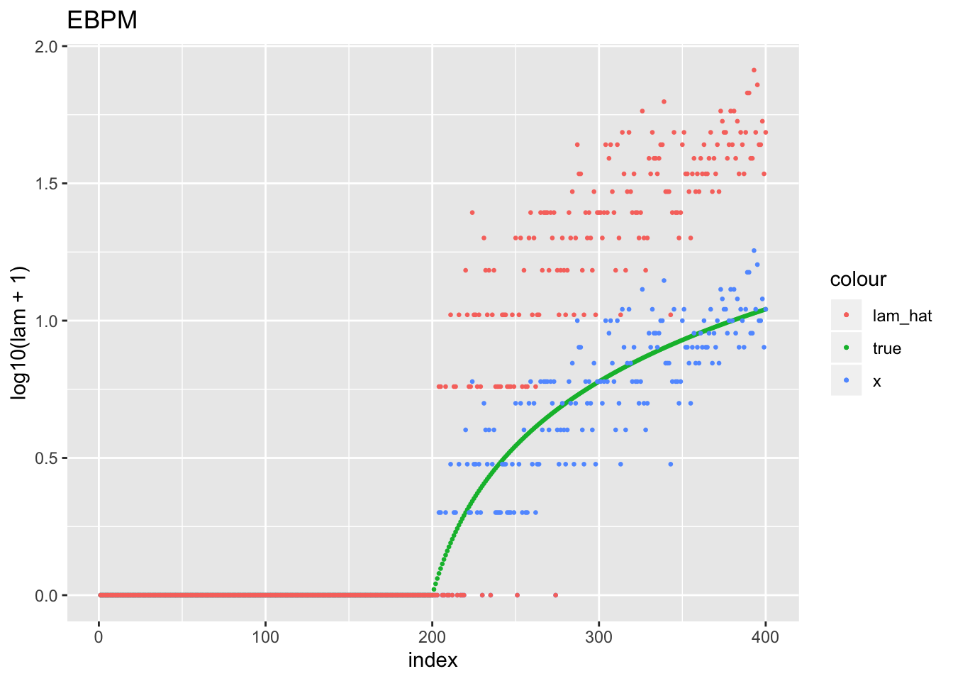
ggplot(df)  + geom_point(aes(x = x, y = lam_hat, color = "blue"), cex = 0.5) +
               labs(x = "x", y = "lam_hat", title = "EBPM") +
               guides(fill = "color")+
                geom_abline(slope = 1)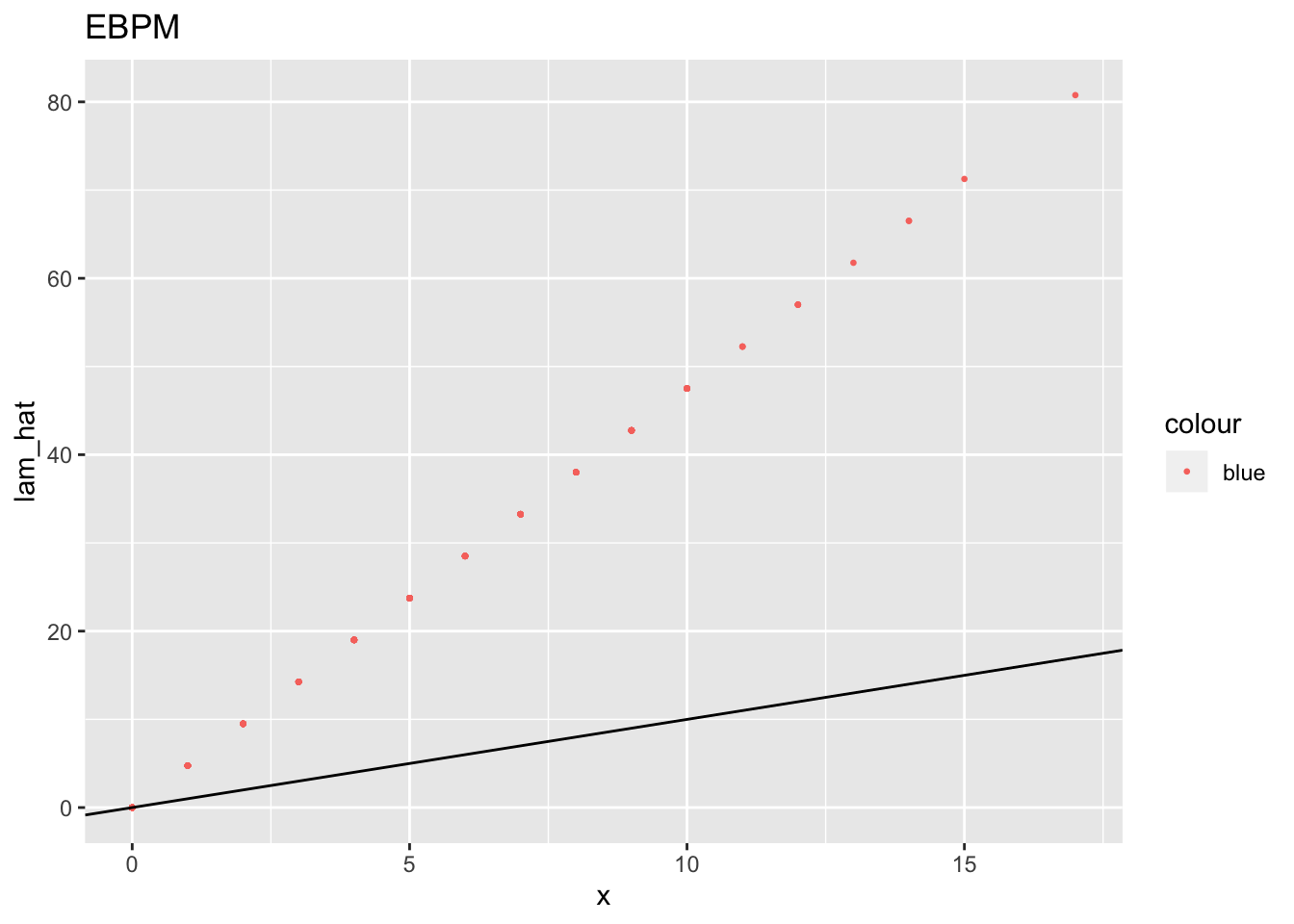
| Version | Author | Date |
|---|---|---|
| 25f8b5a | zihao12 | 2019-09-24 |
lam_true from mixture of gamma (same as grids chosen by the model)
I generate “lam_true” from a mixture of gamma. Then I give the gamma components (grids) to the model. So we can see if the model estimates mixture weights properly
sessionInfo()R version 3.5.1 (2018-07-02)
Platform: x86_64-apple-darwin15.6.0 (64-bit)
Running under: macOS 10.14
Matrix products: default
BLAS: /Library/Frameworks/R.framework/Versions/3.5/Resources/lib/libRblas.0.dylib
LAPACK: /Library/Frameworks/R.framework/Versions/3.5/Resources/lib/libRlapack.dylib
locale:
[1] en_US.UTF-8/en_US.UTF-8/en_US.UTF-8/C/en_US.UTF-8/en_US.UTF-8
attached base packages:
[1] stats graphics grDevices utils datasets methods base
other attached packages:
[1] gtools_3.8.1 ggplot2_3.2.0 mixsqp_0.1-120
loaded via a namespace (and not attached):
[1] Rcpp_1.0.2 compiler_3.5.1 pillar_1.4.1 git2r_0.25.2
[5] workflowr_1.4.0 tools_3.5.1 digest_0.6.19 evaluate_0.14
[9] tibble_2.1.3 gtable_0.3.0 pkgconfig_2.0.2 rlang_0.4.0
[13] yaml_2.2.0 xfun_0.8 withr_2.1.2 stringr_1.4.0
[17] dplyr_0.8.1 knitr_1.23 fs_1.3.1 rprojroot_1.3-2
[21] grid_3.5.1 tidyselect_0.2.5 glue_1.3.1 R6_2.4.0
[25] rmarkdown_1.13 purrr_0.3.2 magrittr_1.5 whisker_0.3-2
[29] backports_1.1.4 scales_1.0.0 htmltools_0.3.6 assertthat_0.2.1
[33] colorspace_1.4-1 labeling_0.3 stringi_1.4.3 lazyeval_0.2.2
[37] munsell_0.5.0 crayon_1.3.4