This reproducible R Markdown analysis was created with workflowr (version 1.2.0). The Report tab describes the reproducibility checks that were applied when the results were created. The Past versions tab lists the development history.
The R Markdown file has unstaged changes. To know which version of the R Markdown file created these results, you’ll want to first commit it to the Git repo. If you’re still working on the analysis, you can ignore this warning. When you’re finished, you can run wflow_publish to commit the R Markdown file and build the HTML.
Great job! The global environment was empty. Objects defined in the global environment can affect the analysis in your R Markdown file in unknown ways. For reproduciblity it’s best to always run the code in an empty environment.
The command set.seed(20181214) was run prior to running the code in the R Markdown file. Setting a seed ensures that any results that rely on randomness, e.g. subsampling or permutations, are reproducible.
Great! You are using Git for version control. Tracking code development and connecting the code version to the results is critical for reproducibility. The version displayed above was the version of the Git repository at the time these results were generated.
Note that you need to be careful to ensure that all relevant files for the analysis have been committed to Git prior to generating the results (you can use wflow_publish or wflow_git_commit). workflowr only checks the R Markdown file, but you know if there are other scripts or data files that it depends on. Below is the status of the Git repository when the results were generated:
Note that any generated files, e.g. HTML, png, CSS, etc., are not included in this status report because it is ok for generated content to have uncommitted changes.
These are the previous versions of the R Markdown and HTML files. If you’ve configured a remote Git repository (see ?wflow_git_remote), click on the hyperlinks in the table below to view them.
In this vignette, we process fastq data from scRNA-seq (10x v2 chemistry) with to make a sparse matrix that can be used in downstream analysis. Then we will start that standard downstream analysis with Seurat.
Setup
First, if you want to run this notebook, please make sure you have git installed, go to the terminal and
This will download a directory called BUS_notebooks_R in the directory you are in when running the git command. Inside the BUS_notebooks_R directory, this notebook is in the analysis directory. Then create an R project in the BUS_notebooks_R directory. Also, in RStudio, go to Tools -> Global Options -> R Markdown, and set “Evaluate chunks in directory” to “Project”. The reason why is that this website was built with workflowr, which renders the notebooks in the project directory rather than the document directory.
Alternatively, you can directly download this notebook here and open it in RStudio, but make sure to adjust the paths where files are downloaded and where output files are stored to match those in your environment.
Install packages
The primary analysis section of this notebook demonstrates the use of command line tools kallisto and bustools. Please use kallisto 0.45, whose binary can be downloaded here. The binary of bustools can be found here.
After you download the binary, you should decompress the file (if it is tar.gz) with tar -xzvf file.tar.gz in the bash terminal, and add the directory containing the binary to PATH by export PATH=$PATH:/foo/bar, where /foo/bar here is the directory of interest. Then you can directly invoke the binary on the command line as we will do in this notebook.
Note for Windows users: bustools does not have a Windows binary, but you can use a Linux subsystem in Windows 10. If you use earlier version of Windows, then unfortunately you need to either use Linux dual boot or virtual machine or find a Linux or Mac computer such as a server.
We will be using the R packages below. BUSpaRse is not yet on CRAN or Bioconductor. For Mac users, see the installation note for BUSpaRse. We will also use Seurat 3.0, which is not yet on CRAN (the CRAN version is 2.3.4), for the standard downstream analysis. Seurat 3.0 has some cool new features such as getting batch corrected gene count matrix and cell label transfer across datasets. See this paper for more detail. Though we will not get into those new features here, it’s worthwhile to check them out.
# Install devtools if it's not already installed
if (!require(devtools)) {
  install.packages("devtools")
}
# Install from GitHub
devtools::install_github("BUStools/BUSpaRse")
devtools::install_github("satijalab/seurat", ref = "release/3.0")
The package DropletUtils will be used to estimate the number of real cells as opposed to empty droplets. It’s on Bioconductor, and here is how it should be installed:
if (!require(BiocManager)) {
  install.packages("BiocManager")
}
BiocManager::install("DropletUtils")
The other R packages below are on CRAN, and can be installed with install.packages.
The data set we are using here is 1k 1:1 Mixture of Fresh Frozen Human (HEK293T) and Mouse (NIH3T3) Cells from the 10x website. First, we download the fastq files (6.34 GB).
Here we use kallisto to pseudoalign the reads to the transcriptome and then to create the bus file to be converted to a sparse matrix. The first step is to build an index of the transcriptome. This data set has both human and mouse cells, so we need both human and mouse transcriptomes. The transcriptomes downloaded here are from Ensembl version 95, released in January 2019. As of the writing of this notebook, this is the most recent Ensembl release.
# Human transcriptome
if (!file.exists("./data/hs_cdna.fa.gz")) {
  download.file("ftp://ftp.ensembl.org/pub/release-95/fasta/homo_sapiens/cdna/Homo_sapiens.GRCh38.cdna.all.fa.gz", "./data/hs_cdna.fa.gz", method = "wget", quiet = TRUE)
}
# Mouse transcriptome
if (!file.exists("./data/mm_cdna.fa.gz")) {
  download.file("ftp://ftp.ensembl.org/pub/release-95/fasta/mus_musculus/cdna/Mus_musculus.GRCm38.cdna.all.fa.gz", "./data/mm_cdna.fa.gz", method = "wget", quiet = TRUE)
}
kallisto version
#> kallisto, version 0.45.0
Actually, we don’t need to unzip the fasta files
kallisto index -i ./output/hs_mm_tr_index.idx ./data/hs_cdna.fa.gz ./data/mm_cdna.fa.gz
#>
#> [build] loading fasta file ./data/hs_cdna.fa.gz
#> [build] loading fasta file ./data/mm_cdna.fa.gz
#> [build] k-mer length: 31
#> [build] warning: clipped off poly-A tail (longer than 10)
#>         from 2083 target sequences
#> [build] warning: replaced 8 non-ACGUT characters in the input sequence
#>         with pseudorandom nucleotides
#> [build] counting k-mers ... done.
#> [build] building target de Bruijn graph ...  done
#> [build] creating equivalence classes ...  done
#> [build] target de Bruijn graph has 2145397 contigs and contains 206575877 k-mers
Run kallisto bus
Here we will generate the bus file. Here bus stands for Barbode, UMI, Set (i.e. equivalent class). In text form, it is a table whose first column is the barcode. The second column is the UMI that are associated with the barcode. The third column is the index of the equivalence class reads with the UMI maps to (equivalence class will be explained later). The fourth column is count of reads with this barcode, UMI, and equivalence class combination, which is ignored as one UMI should stand for one molecule. See this paper for more detail.
These are the technologies supported by kallisto bus:
system("kallisto bus --list", intern = TRUE)
#> Warning in system("kallisto bus --list", intern = TRUE): running command
#> 'kallisto bus --list' had status 1
Here we have 8 samples. Each sample has 3 files: I1 means sample index, R1 means barcode and UMI, and R2 means the piece of cDNA. The -i argument specifies the index file we just built. The -o argument specifies the output directory. The -x argument specifies the sequencing technology used to generate this data set. The -t argument specifies the number of threads used. I ran this on a server and used 8 threads.
#>
#> [index] k-mer length: 31
#> [index] number of targets: 303,693
#> [index] number of k-mers: 206,575,877
#> [index] number of equivalence classes: 1,256,267
#> [quant] will process sample 1: ./fastqs/hgmm_1k_S1_L001_R1_001.fastq.gz
#>                                ./fastqs/hgmm_1k_S1_L001_R2_001.fastq.gz
#> [quant] will process sample 2: ./fastqs/hgmm_1k_S1_L002_R1_001.fastq.gz
#>                                ./fastqs/hgmm_1k_S1_L002_R2_001.fastq.gz
#> [quant] will process sample 3: ./fastqs/hgmm_1k_S1_L003_R1_001.fastq.gz
#>                                ./fastqs/hgmm_1k_S1_L003_R2_001.fastq.gz
#> [quant] will process sample 4: ./fastqs/hgmm_1k_S1_L004_R1_001.fastq.gz
#>                                ./fastqs/hgmm_1k_S1_L004_R2_001.fastq.gz
#> [quant] will process sample 5: ./fastqs/hgmm_1k_S1_L005_R1_001.fastq.gz
#>                                ./fastqs/hgmm_1k_S1_L005_R2_001.fastq.gz
#> [quant] will process sample 6: ./fastqs/hgmm_1k_S1_L006_R1_001.fastq.gz
#>                                ./fastqs/hgmm_1k_S1_L006_R2_001.fastq.gz
#> [quant] will process sample 7: ./fastqs/hgmm_1k_S1_L007_R1_001.fastq.gz
#>                                ./fastqs/hgmm_1k_S1_L007_R2_001.fastq.gz
#> [quant] will process sample 8: ./fastqs/hgmm_1k_S1_L008_R1_001.fastq.gz
#>                                ./fastqs/hgmm_1k_S1_L008_R2_001.fastq.gz
#> [quant] finding pseudoalignments for the reads ... done
#> [quant] processed 63,252,296 reads, 52,231,469 reads pseudoaligned
The output.bus file is a binary. In order to make R parse it, we need to convert it into a sorted text file. There’s a command line tool bustools for this. The reason why kallisto bus outputs this binary rather than the sorted text file directly is that the binary can be very compressed to save disk space. The such compression is achieved, a future version of R package BUSpaRse may support directly reading the binary to convert to sparse matrix. At present, as bustools is still under development, such compression has not been achieved, and as a result, the binary is slightly larger than the text file.
# Add where I installed bustools to PATH
export PATH=$PATH:/home/lambda/mylibs/bin/
# Sort, with 8 threads
bustools sort -o ./output/out_hgmm1k/output.sorted -t8 ./output/out_hgmm1k/output.bus
# Convert sorted file to text
bustools text -o ./output/out_hgmm1k/output.sorted.txt ./output/out_hgmm1k/output.sorted
#> Read in 52231469 number of busrecords
#> All sorted
#> Read in 43778790 number of busrecords
This is what the bus file looks like:
First column is barcode, second column is UMI, 3rd column is equivalence class index, and 4th column is count, which is ignored. This has already been sorted according to barcode.
For the sparse matrix, most people are interested in how many UMIs per gene per cell, we here we will quantify this from the bus output, and to do so, we need to find which gene corresponds to each transcript. Remember in the output of kallisto bus, there’s the file transcripts.txt. Those are the transcripts in the transcriptome index. Now we’ll only keep the transcripts present there and make sure that the transcripts in tr2g are in the same order as those in the index. You will soon see why the order is important.
Remember that we downloaded transcriptome FASTA files from Ensembl just now. In FASTA files, each entry is a sequence with a name. In Ensembl FASTA files, the sequence name has genome annotation of the corresponding sequence, so we can extract transcript IDs and corresponding gene IDs and gene names from there.
Alternative ways of getting tr2g have been implemented in the BUSpaRse package. You may use tr2g_ensembl to query Ensembl with biomart to get transcript and gene IDs. If you use this method, then please make sure that the Ensembl version used in the query matches that of the transcriptome. This method is convenient for the user since you only need to input species names, but it can be slow since biomart database query can be slow. You may also use tr2g_gtf for GTF files and tr2g_gff3 for GFF3 files, which are more useful for non-model organisms absent from Ensemble. After calling the tr2g_* family of functions, you should sort the transcripts from those functions with sort_tr2g so the transcripts are in the same order as those in the kallisto index. The FASTA way is the fastest, as reading FASTA files is faster than reading GTF and GFF files. Whichever way you choose, this shouldn’t take much more than half a minute per species.
The function transcript2gene not only gets the transcript and gene IDs but also sorts the transcripts. This function only supports Ensembl biomart query and Ensembl fasta files as the source of transcript and gene IDs, as the attribute field of GTF and GFF3 files can differ between sources and further cleanup may be needed.
Make the sparse matrix
For 10x, we do have a file with all valid cell barcodes that comes with CellRanger. You need to install CellRanger to get this file, though you do not need to run CellRanger for this notebook. The whitelist is optional, so if you don’t have one, you may skip the whitelist step and the whitelist argument in the makr_sparse_matrix function.
# Copy v2 chemistry whitelist to working directory
cp ~/cellranger-3.0.1/cellranger-cs/3.0.1/lib/python/cellranger/barcodes/737K-august-2016.txt \
./data/whitelist_v2.txt
# Read in the whitelist
whitelist_v2 <- fread("./data/whitelist_v2.txt", header = FALSE)$V1
length(whitelist_v2)
#> [1] 737280
There about 737K valid cell barcodes.
Now we have everything we need to make the sparse matrix. This function reads in output.sorted.txt line by line and processes them. It does not do barcode correction for now, so the barcode must exactly match those in the whitelist if one is provided. It took 5 to 6 minutes to construct the sparse matrix in the hgmm6k dataset, which has over 280 million lines in output.sorted.txt, which is over 9GB. Here the data set is smaller, and it takes less than a minute. A future version of BUSpaRse will parallelize this process to make it more scalable for huge datasets. For now, it’s single threaded.
Note that the arguments est_ncells (estimated number of cells) and est_ngenes (estimated number of genes) are important. With the estimate, this function reserves memory for the data to be added into, reducing the need of reallocation, which will slow the function down. Since the vast majority of “cells” you get in this sparse matrix are empty droplets rather than cells, please put at least 200 times more “cells” than you actually expect in est_ncells.
If you do not have a whitelist of barcodes, then it’s fine; the whitelist argument is optional.
The function make_sparse_matrix can make the gene count matrix and the transcript compatibility count (TCC) matrix at the same time. For the purpose of this notebook, we only generate the gene count matrix. An upcoming notebook will demonstrate some more detailed analysis with a TCC matrix. See Ntranos et al. 2016 for more information about TCC matrices.
#> Reading matrix.ec
#> Processing ECs
#> Matching genes to ECs
#> Reading data
#> Read 5 million reads
#> Read 10 million reads
#> Read 15 million reads
#> Read 20 million reads
#> Read 25 million reads
#> Read 30 million reads
#> Read 35 million reads
#> Read 40 million reads
#> Constructing gene count matrix
The matrix we get has genes in rows and barcode in columns. The row names are the gene IDs (not using human readable gene names since they’re not guaranteed to be unique), and the column names are cell barcodes.
For Ensembl transcriptomes, you may call busparse_matrix to bypass the separate step of getting the tr2g data frame here to directly get the matrix.
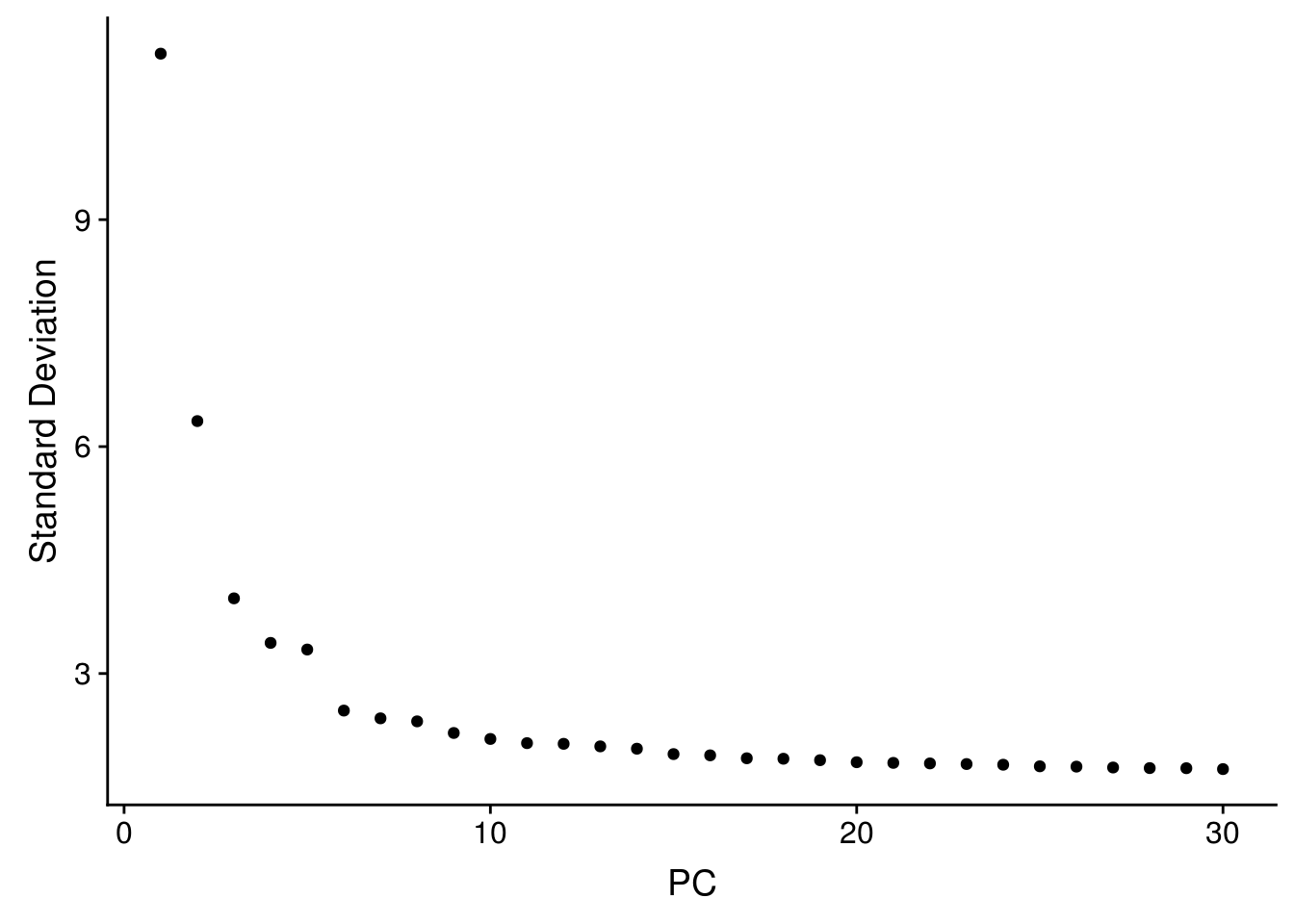
Explore the data
Remove empty droplets
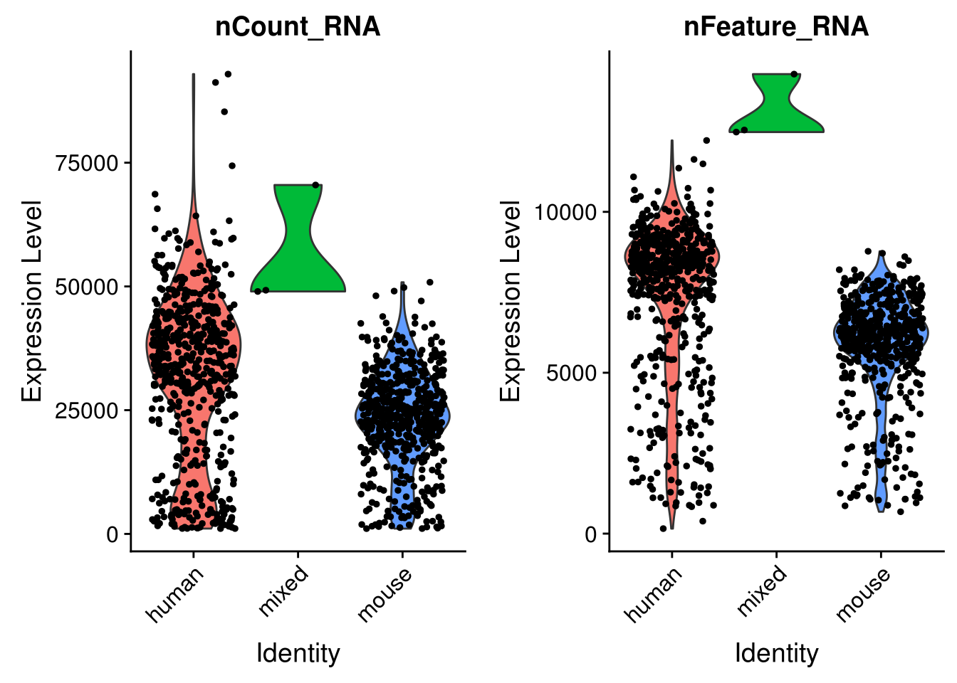
Cool, so now we have the sparse matrix. What does it look like?
dim(res_mat)
#> [1] 47367 353961
That’s way more cells than we expect, which is about 1000. So what’s going on?
#>    Min. 1st Qu.  Median    Mean 3rd Qu.    Max.
#>     1.0     1.0     2.0   101.8    11.0 92917.0
The vast majority of “cells” have only a few UMI detected. Those are empty droplets. 10x claims to have cell capture rate of up to 65%, but in practice, depending on how many cells are in fact loaded, the rate can be much lower. A commonly used method to estimate the number of empty droplets is barcode ranking knee and inflection points, as those are often assumed to represent transition between two components of a distribution. While more sophisticated method exist (e.g. see emptyDrops in DropletUtils), for simplicity, we will use the barcode ranking method here. However, whichever way we go, we don’t have the ground truth.
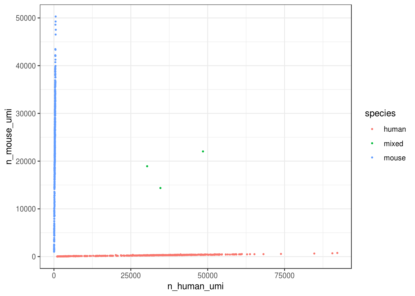
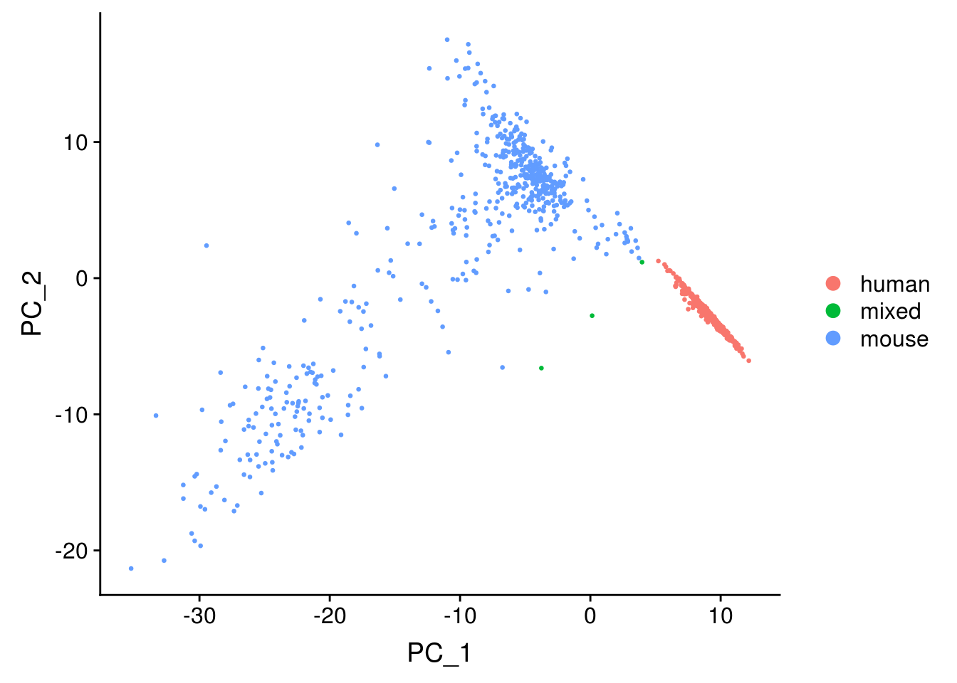
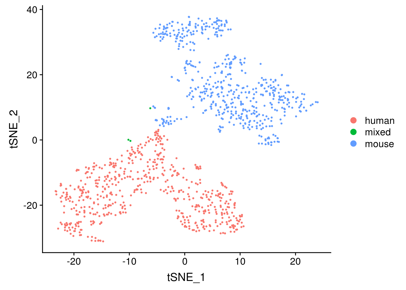
Great, looks like the vast majority of cells are not mixed.
cell_species %>%
  dplyr::count(species) %>%
  mutate(proportion = n / ncol(res_mat))
#> # A tibble: 3 x 3
#>   species     n proportion
#>   <chr>   <int>      <dbl>
#> 1 human     579    0.516
#> 2 mixed       3    0.00267
#> 3 mouse     541    0.482
Great, only about 0.3% of cells here are doublets, which is lower than the ~1% 10x lists. Doublet rate tends to be lower when cell concentration is lower. However, doublets can still be formed with cells from the same species, so the number of mixed species “cells” is only a lower bound of doublet rate.