Figure 3
Nils Eling and Nicolas Damond
2020-07-10
Last updated: 2020-07-10
Checks: 6 1
Knit directory: cytomapper_publication/
This reproducible R Markdown analysis was created with workflowr (version 1.6.2). The Checks tab describes the reproducibility checks that were applied when the results were created. The Past versions tab lists the development history.
The R Markdown file has unstaged changes. To know which version of the R Markdown file created these results, you’ll want to first commit it to the Git repo. If you’re still working on the analysis, you can ignore this warning. When you’re finished, you can run wflow_publish to commit the R Markdown file and build the HTML.
Great job! The global environment was empty. Objects defined in the global environment can affect the analysis in your R Markdown file in unknown ways. For reproduciblity it’s best to always run the code in an empty environment.
The command set.seed(20200602) was run prior to running the code in the R Markdown file. Setting a seed ensures that any results that rely on randomness, e.g. subsampling or permutations, are reproducible.
Great job! Recording the operating system, R version, and package versions is critical for reproducibility.
Nice! There were no cached chunks for this analysis, so you can be confident that you successfully produced the results during this run.
Great job! Using relative paths to the files within your workflowr project makes it easier to run your code on other machines.
Great! You are using Git for version control. Tracking code development and connecting the code version to the results is critical for reproducibility.
The results in this page were generated with repository version 75c032f. See the Past versions tab to see a history of the changes made to the R Markdown and HTML files.
Note that you need to be careful to ensure that all relevant files for the analysis have been committed to Git prior to generating the results (you can use wflow_publish or wflow_git_commit). workflowr only checks the R Markdown file, but you know if there are other scripts or data files that it depends on. Below is the status of the Git repository when the results were generated:
Ignored files:
    Ignored:    .DS_Store
    Ignored:    .Rhistory
    Ignored:    .Rproj.user/
    Ignored:    analysis/.DS_Store
    Ignored:    data/PancreasData/.DS_Store
    Ignored:    data/PancreasData/pancreas_images.rds
    Ignored:    data/PancreasData/pancreas_masks.rds
    Ignored:    data/PancreasData/pancreas_sce.rds

Unstaged changes:
    Modified:   analysis/03-Figure_3.Rmd
    Modified:   analysis/03-Figure_4.Rmd
Note that any generated files, e.g. HTML, png, CSS, etc., are not included in this status report because it is ok for generated content to have uncommitted changes.
These are the previous versions of the repository in which changes were made to the R Markdown (analysis/03-Figure_3.Rmd) and HTML (docs/03-Figure_3.html) files. If you’ve configured a remote Git repository (see ?wflow_git_remote), click on the hyperlinks in the table below to view the files as they were in that past version.
| File | Version | Author | Date | Message |
|---|---|---|---|---|
| html | a100544 | nilseling | 2020-07-10 | Recompiled htmls |
| html | 2e3df83 | nilseling | 2020-07-09 | Added Github icon and recompiled |
| html | 69f1501 | nilseling | 2020-07-09 | Small fixes and recompilation |
| Rmd | 86ddc2d | nilseling | 2020-07-09 | Increased figure size for reporting |
| html | 86ddc2d | nilseling | 2020-07-09 | Increased figure size for reporting |
| html | 5476a61 | nilseling | 2020-07-08 | Recompiled files |
| Rmd | cb92024 | nilseling | 2020-07-03 | Finalized Figure 4 |
| html | cb92024 | nilseling | 2020-07-03 | Finalized Figure 4 |
| Rmd | 9b40183 | nilseling | 2020-07-03 | Finalized Figure 3 |
This script reproduces the analysis performed in Figure 3. Here, we will load the libraries and data for this figure:
library(cytomapper)
library(dplyr)

sce <- readRDS("data/PancreasData/pancreas_sce.rds")
masks <- readRDS("data/PancreasData/pancreas_masks.rds")
We will now order the images based on the percentage of beta cells out of all islet cells. In that way, we can visualize the decline of beta cells across all sample images.
cur_summary <- as_tibble(colData(sce)) %>%
  # Calculate for each image the area and beta cell density
  group_by(ImageNumber) %>%
  summarise(ImageName = unique(ImageName),
            Stage = unique(stage),
            betaCellCount = sum(CellType == "beta"),
            isletCellCount = sum(CellCat == "islet")) %>%
  mutate(betaCellFraction = betaCellCount / isletCellCount) %>%
  arrange(desc(betaCellFraction))
`summarise()` ungrouping output (override with `.groups` argument)Next, we will plot the cell-types on images after reordering them by beta cell fraction. We will further subset the SingleCellExperiment object to only contain iselt cells.
cur_sce <- sce[,sce$CellCat == "islet"]
cur_order <- match(cur_summary$ImageName, mcols(masks)$ImageName)

# Define the colors for the different cell types
ct_colours <- vector(mode = "character", length = length(unique(cur_sce$CellType)))
names(ct_colours) <- unique(cur_sce$CellType)
ct_colours["beta"] <- "yellow"
ct_colours["alpha"] <- "firebrick1"
ct_colours["delta"] <- "firebrick3"
ct_colours["gamma"] <- "deeppink4"

plotCells(mask = masks[cur_order],
          object = cur_sce,
          img_id = "ImageName",
          cell_id = "CellNumber",
          colour_by = "CellType",
          scale_bar = list(length = 100,
                           label = "",
                           colour = "black"),
          legend = list(margin = 100),
          colour = list(CellType = ct_colours),
          missing_colour = "white",
          background_colour = "gray",
          image_title = list(text = paste(cur_summary$ImageName, "-",
                                          cur_summary$Stage),
                             colour = "black"))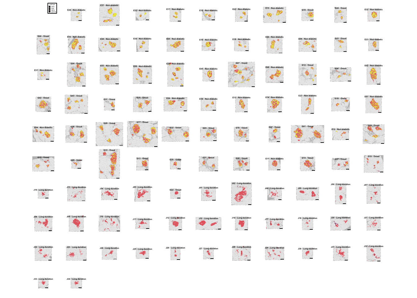
# Save plot
plotCells(mask = masks[cur_order],
          object = cur_sce,
          img_id = "ImageName",
          cell_id = "CellNumber",
          colour_by = "CellType",
          scale_bar = list(length = 100,
                           label = "",
                           colour = "black"),
          legend = list(colour_by.legend.cex = 9,
                        margin = 100),
          colour = list(CellType = ct_colours),
          missing_colour = "white",
          background_colour = "gray",
          image_title = list(text = paste(cur_summary$ImageName, "-",
                                          cur_summary$Stage),
                             colour = "black"),
          save_plot = list(filename = "docs/final_figures/main/Fig_3.png"))
Here, we see the progressive decline in beta cell fractions. The images are ordered based on T1D stage: Non-diabetic, Onset and Long-Duration, as expected. We further see an increased morphological irregularity in Long-Duration islets.
sessionInfo()R version 4.0.0 (2020-04-24)
Platform: x86_64-apple-darwin17.0 (64-bit)
Running under: macOS Catalina 10.15.5
Matrix products: default
BLAS: /Library/Frameworks/R.framework/Versions/4.0/Resources/lib/libRblas.dylib
LAPACK: /Library/Frameworks/R.framework/Versions/4.0/Resources/lib/libRlapack.dylib
locale:
[1] en_US.UTF-8/en_US.UTF-8/en_US.UTF-8/C/en_US.UTF-8/en_US.UTF-8
attached base packages:
[1] parallel stats4 stats graphics grDevices utils datasets
[8] methods base
other attached packages:
[1] dplyr_1.0.0 cytomapper_1.1.1
[3] SingleCellExperiment_1.10.1 SummarizedExperiment_1.18.1
[5] DelayedArray_0.14.0 matrixStats_0.56.0
[7] Biobase_2.48.0 GenomicRanges_1.40.0
[9] GenomeInfoDb_1.24.2 IRanges_2.22.2
[11] S4Vectors_0.26.1 BiocGenerics_0.34.0
[13] EBImage_4.30.0 workflowr_1.6.2
loaded via a namespace (and not attached):
[1] Rcpp_1.0.4.6 locfit_1.5-9.4 lattice_0.20-41
[4] fftwtools_0.9-8 png_0.1-7 rprojroot_1.3-2
[7] digest_0.6.25 R6_2.4.1 tiff_0.1-5
[10] backports_1.1.7 evaluate_0.14 ggplot2_3.3.1
[13] pillar_1.4.4 zlibbioc_1.34.0 rlang_0.4.6
[16] whisker_0.4 raster_3.1-5 Matrix_1.2-18
[19] rmarkdown_2.2 stringr_1.4.0 htmlwidgets_1.5.1
[22] RCurl_1.98-1.2 munsell_0.5.0 compiler_4.0.0
[25] httpuv_1.5.4 xfun_0.14 pkgconfig_2.0.3
[28] htmltools_0.4.0 tidyselect_1.1.0 gridExtra_2.3
[31] tibble_3.0.1 GenomeInfoDbData_1.2.3 codetools_0.2-16
[34] viridisLite_0.3.0 crayon_1.3.4 later_1.1.0.1
[37] bitops_1.0-6 grid_4.0.0 gtable_0.3.0
[40] lifecycle_0.2.0 git2r_0.27.1 magrittr_1.5
[43] scales_1.1.1 stringi_1.4.6 XVector_0.28.0
[46] viridis_0.5.1 fs_1.4.1 promises_1.1.1
[49] sp_1.4-2 generics_0.0.2 ellipsis_0.3.1
[52] vctrs_0.3.1 RColorBrewer_1.1-2 tools_4.0.0
[55] glue_1.4.1 purrr_0.3.4 jpeg_0.1-8.1
[58] abind_1.4-5 yaml_2.2.1 colorspace_1.4-1
[61] knitr_1.28