This reproducible R Markdown analysis was created with workflowr (version 1.6.2). The Checks tab describes the reproducibility checks that were applied when the results were created. The Past versions tab lists the development history.
Great job! The global environment was empty. Objects defined in the global environment can affect the analysis in your R Markdown file in unknown ways. For reproduciblity it’s best to always run the code in an empty environment.
The command set.seed(20200930) was run prior to running the code in the R Markdown file. Setting a seed ensures that any results that rely on randomness, e.g. subsampling or permutations, are reproducible.
Great! You are using Git for version control. Tracking code development and connecting the code version to the results is critical for reproducibility.
The results in this page were generated with repository version 154ffc2. See the Past versions tab to see a history of the changes made to the R Markdown and HTML files.
Note that you need to be careful to ensure that all relevant files for the analysis have been committed to Git prior to generating the results (you can use wflow_publish or wflow_git_commit). workflowr only checks the R Markdown file, but you know if there are other scripts or data files that it depends on. Below is the status of the Git repository when the results were generated:
Note that any generated files, e.g. HTML, png, CSS, etc., are not included in this status report because it is ok for generated content to have uncommitted changes.
These are the previous versions of the repository in which changes were made to the R Markdown (analysis/dge_analysis.Rmd) and HTML (docs/dge_analysis.html) files. If you’ve configured a remote Git repository (see ?wflow_git_remote), click on the hyperlinks in the table below to view the files as they were in that past version.
Annotation data was loaded as an EnsDb object, using Ensembl release 101. Transcript level gene lengths and GC content was converted to gene level values using:
GC Content: The total GC content divided by the total length of transcripts
pander(
  mergedSamples,
  caption = "*Summary of sequencing total runs for all samples*"
)
Summary of sequencing total runs for all samples
name
rep
treat
n
MFM1-D
1
DHT
8
MFM1-V
1
Vehicle
8
MFM2-D
2
DHT
8
MFM3-D
3
DHT
8
MFM3-V
3
Vehicle
8
MFM4-D
4
DHT
8
MFM4-V
4
Vehicle
8
MFM5-D
5
DHT
8
MFM5-V
5
Vehicle
8
MFM6-D
6
DHT
8
MFM6-V
6
Vehicle
8
This data set is slightly unique in that samples were sequenced across multiple lanes and flowcells. Metadata was re-organised to enable summarising of counts across the multiple sequencing runs obtained for every sample. The initial PCA showed that variability between replicates and flowcells was dwarfed by variability between samples. As such, all counts were able to be merged to give a single set of counts for each individual sample.
Importantly, no control (Vehicle) sample was found for replicate 2 and if using a nested approach this treated sample may need to be omitted
The criteria for a gene to be considered as detected, \(>\) 1.5 counts per million (CPM) were required to observed in \(\geq\) 5.5 samples. This effectively ensured \(\geq\) 10 counts in at least 5.5 merged libraries.
Of the 60,671 genes contained in the annotation for this release, 45,019 genes were removed as failing this criteria for detection, leaving 15,652 genes for downstream analysis.
Distributions of logCPM values on merged counts, A) before and B) after filtering of undetectable genes. Some differences between replicates wre noted.
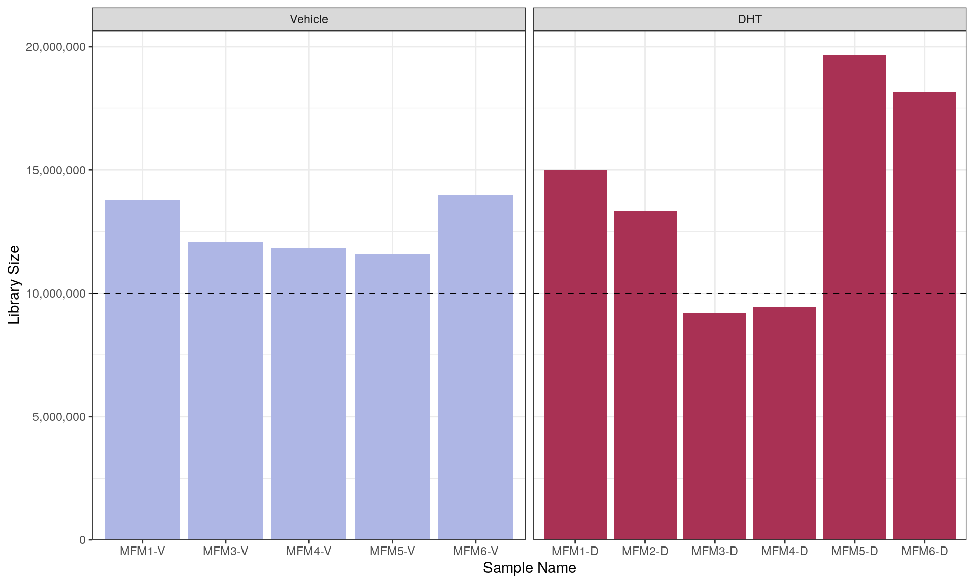
Given that previous work had only assessed the libraries prior to merging, the library sizes were checked after merging replicate sequencing runs. The median library size was found to be 13.3 million reads which is just above the common-use minimum recommendation of 10 million reads/sample.
However, samples MFM3-D and MFM4-D were both below the common-use minimum library size.
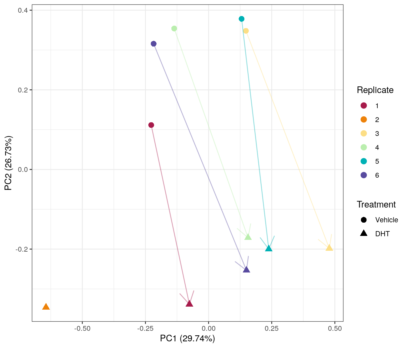
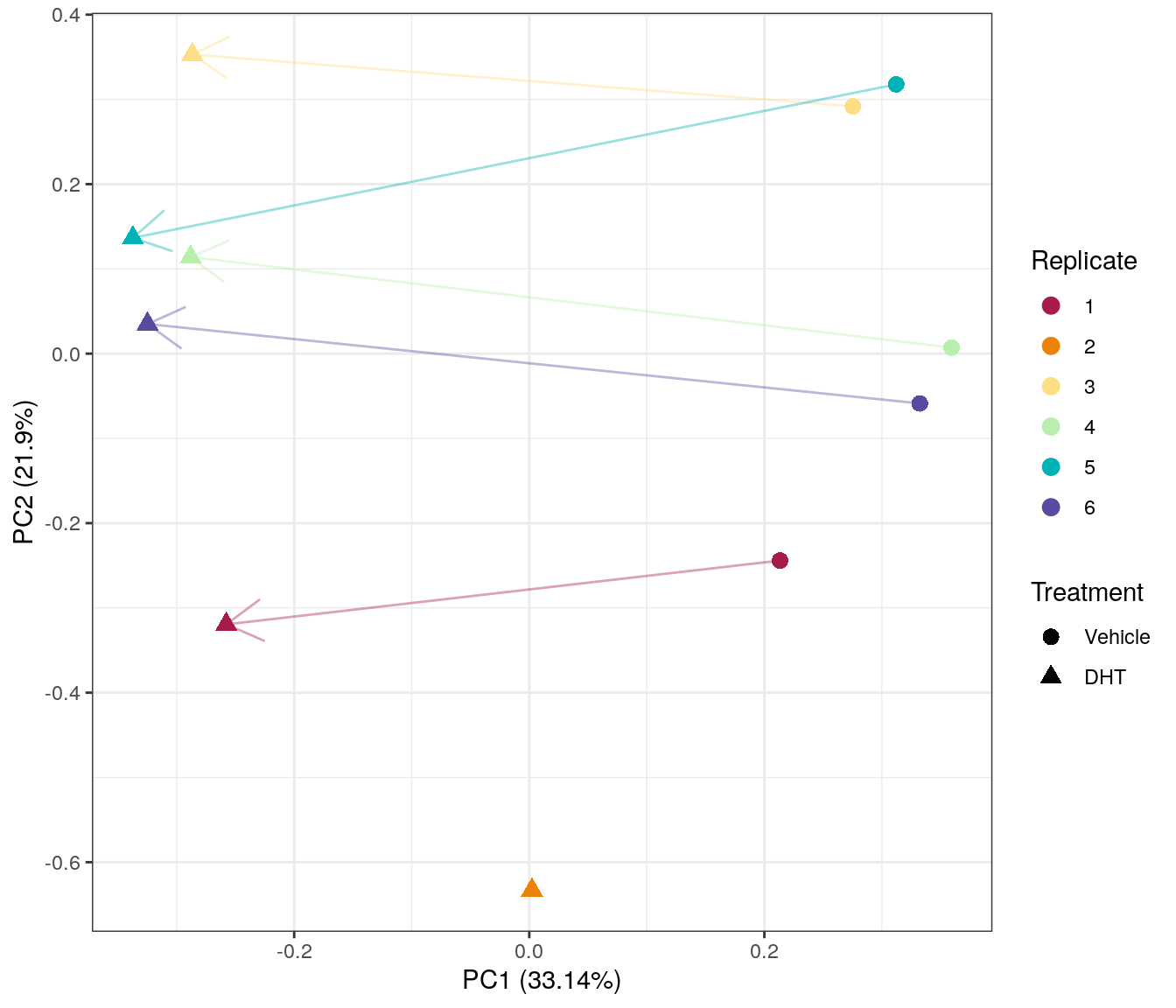
PCA on logCPM from merged counts. PC1 appears to capture the variability between replicates, whilst PC2 primarily captures the effect of DHT treatment. Replicate 2, whch is missing the control sample appears to be the most divergent from the remaining samples.
Despite concerns raised by the library sizes, replicates 3 and 4 appears to be relatively consistent with other samples of the same treatment group.
Checks for GC and Length bias
Given the clear unexpected variability captured by PC1, the impact of GC content or length bias was assessed as a possible source.
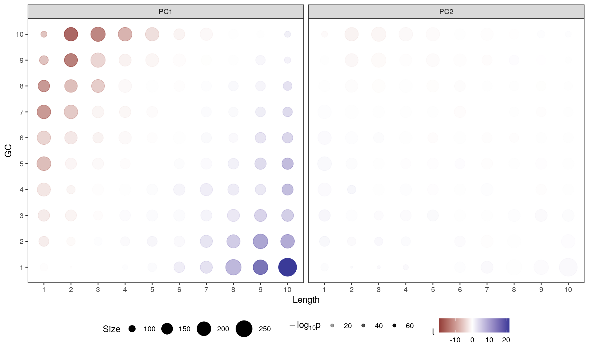
Genes were divided in 10 approximately equal sized bins based on increasing length, and 10 approximately equal sized bins based on increasing GC content, with the final GC/Length bins being the combination 100 bins using both sets. The contribution of each gene to PC1 and PC2 was assessed and a t-test performed on each bin. This tests
where \(\mu\) represents the true contribution to PC1 of all genes in that bin.
If any bin makes a contribution to PC1 the mean will be clearly non-zero, whilst if there is no contribution the mean will be near zero. In this way, the impact of gene length and GC content on variance within the dataset can be assessed. As seen below, the contribution of GC content and gene length to PC1 is very clear, with a smaller contribution being evident across PC2. As a result, Conditional Quantile Normalisation (CQN) is recommended in preference to the more common TMM normalisation.
Contribution of each GC/Length Bin to PC1 and PC2. Fill colours indicate the t-statistic, with tranparency denoting significance as -log10(p), using Bonferroni-adjusted p-values. The number of genes in each bin is indicated by the circle size. The clear pattern across PC1 is unambiguous.
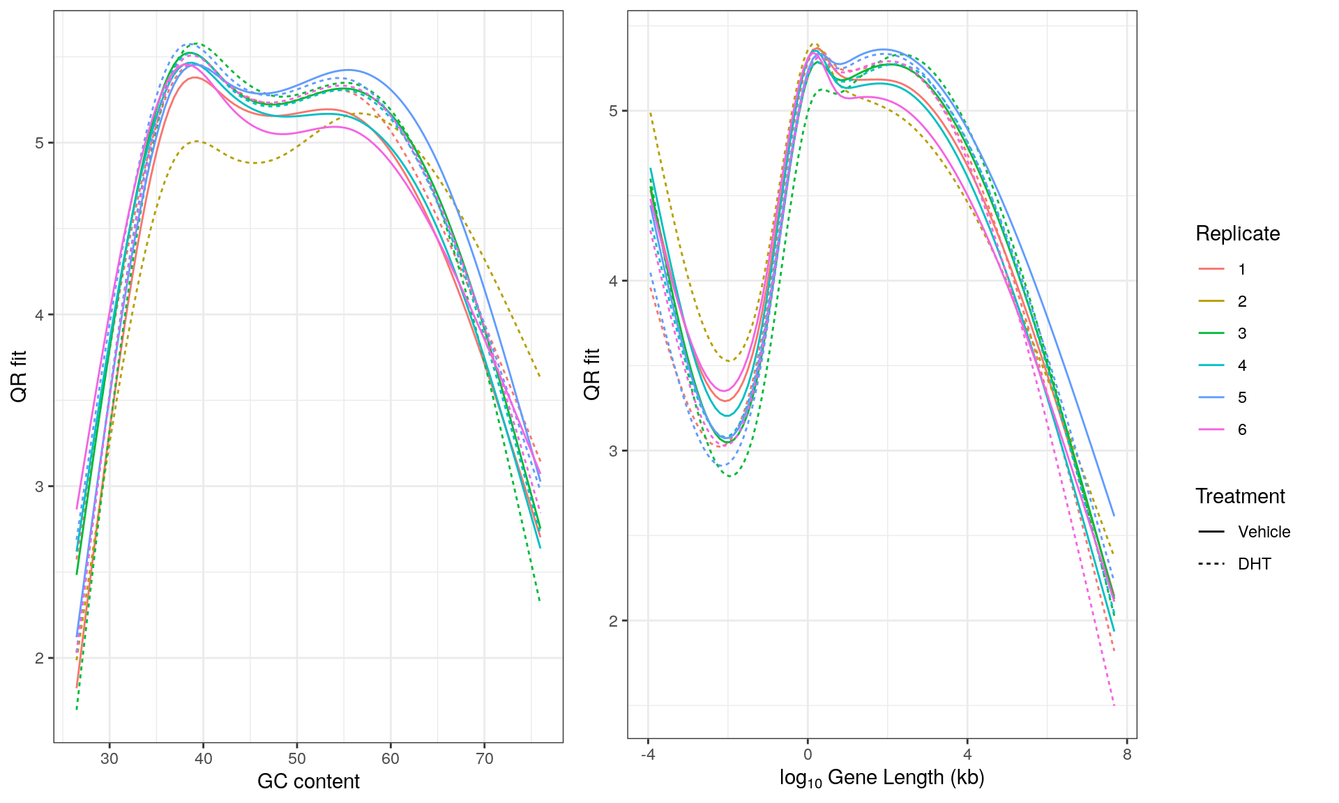
Model fits used when applying CQN. The divergent samples previously noted on the PCA are again quite divergent here. In particular, the long genes with low GC content appear to be where the primary differences are found, in keeping with the previous PCA analysis.
PCA on logCPM after performing CQN. It is immediately apparent the CQN has removed much of the previous PC1, leaving the post-normalised PC1 capturing the majority of the variability. However, replicate 2 appears to be a notable outlier and removal of this ‘orphaned’ treated sample may be required.
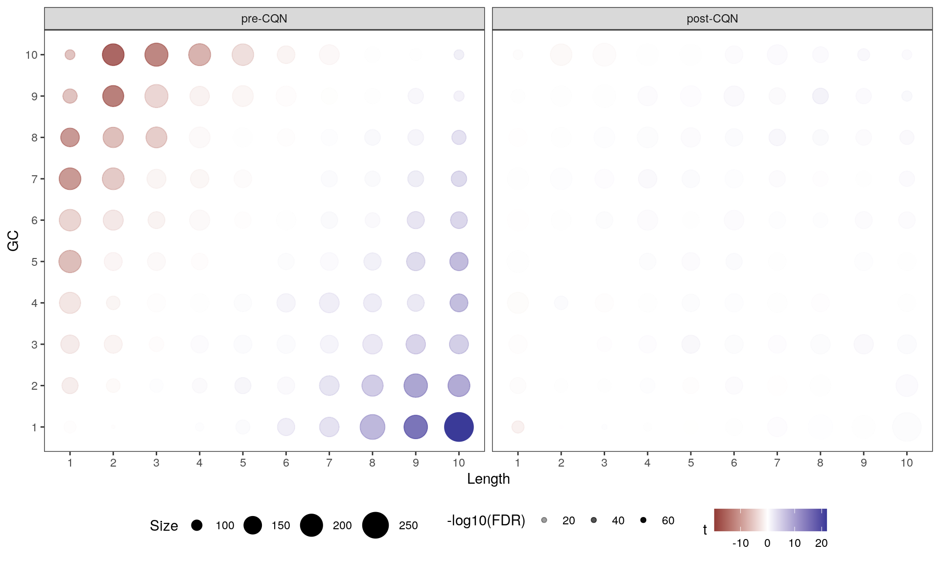
Contributions of gene length and GC content to PC1 shown both before and after CQN. The strong patterns seen before normalisation have clearly been reduced. Fill colours indicate the t-statistic, with tranparency denoting significance as -log10(p), using Bonferroni-adjusted p-values. The number of genes in each bin is indicated by the circle size. The clear pattern across PC1 is unambiguous.
CQN clearly had a positive impact on the data, however, replicate 2 was removed in order to allow the use of a blocking approach, where an individual baseline level is set for each untreated sample and the common difference between vehicle and DHT-treated is then found.
A design matrix was formed giving each replicate it’s own baseline and the common DHT response was then specified as the final column. Following this, dispersions were estimated for the main DGEList object and the model fitted using the Quasi-likelihood GLM.
X <- model.matrix(~0 + rep + treat, data = dge$samples) %>%
  set_colnames(str_remove(colnames(.), "treat"))
dge <- estimateDisp(dge, design = X, robust = TRUE)
fit <- glmQLFit(dge)
In order to detect genes which respond to DHT the Null Hypothesis (\(H_0\)) was specified to be a range around zero, instead of the conventional point-value.
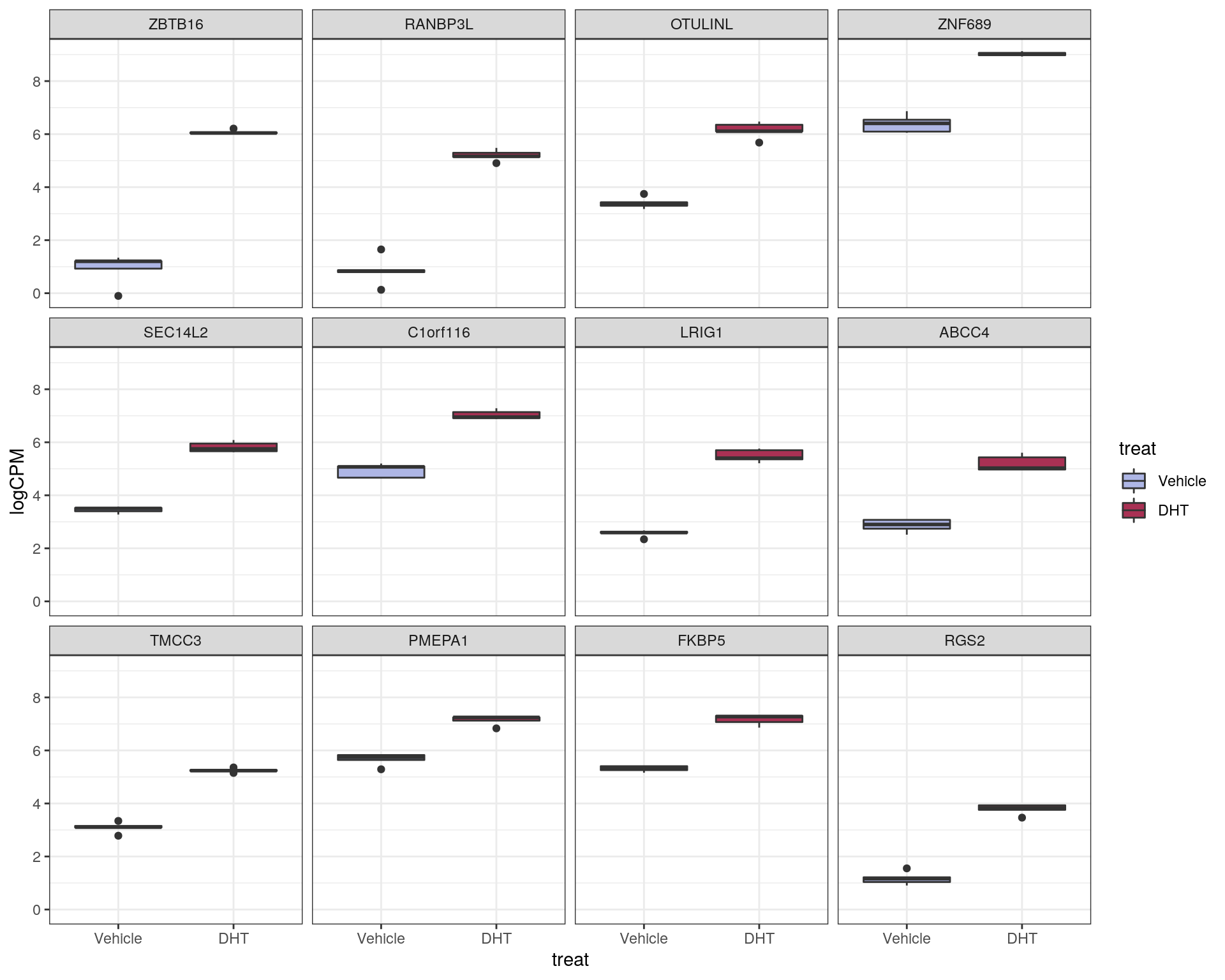
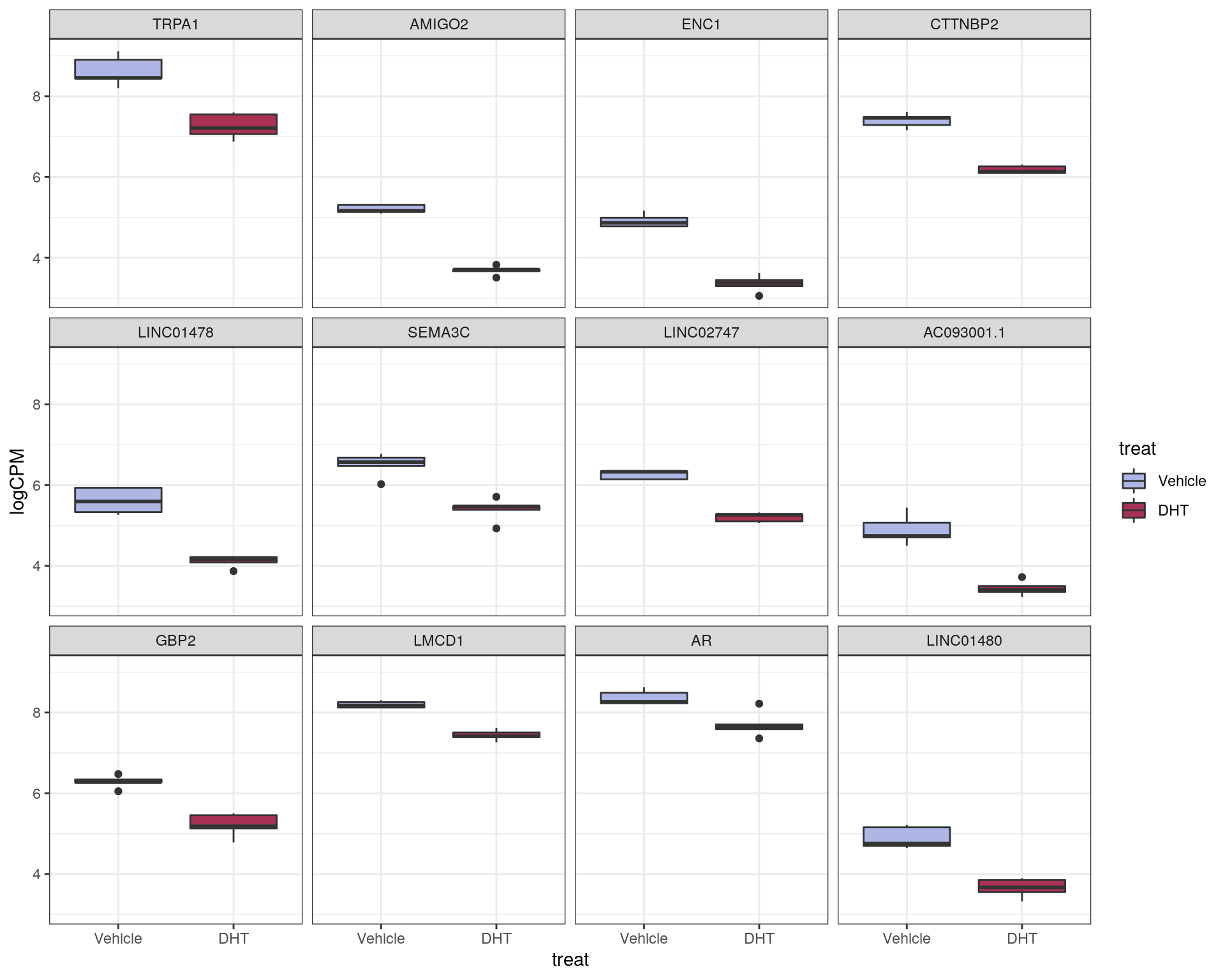
This characterises \(H_0\) as being a range instead of being the singularity 0, with \(\mu\) representing the true mean logFC. The default value of \(\lambda = \log_2 1.2 = 0.263\) was chosen. This removes any requirement for post hoc filtering based on logFC. Using this approach, 856 genes were considered as DE to an FDR of 0.05. Of these, 384 were up-regulated with the remaining 472 being down-regulated.
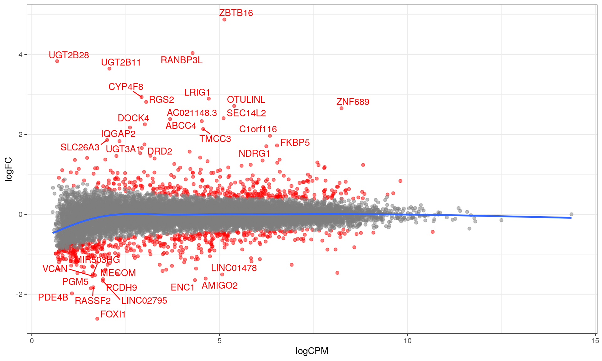
MA plot with blue curve through the data showing the GAM fit. The curve for low-expressed genes indicated a potential bias remains in the data, whilst this is not evident for highly expressed genes. DE genes are highlighted in red.
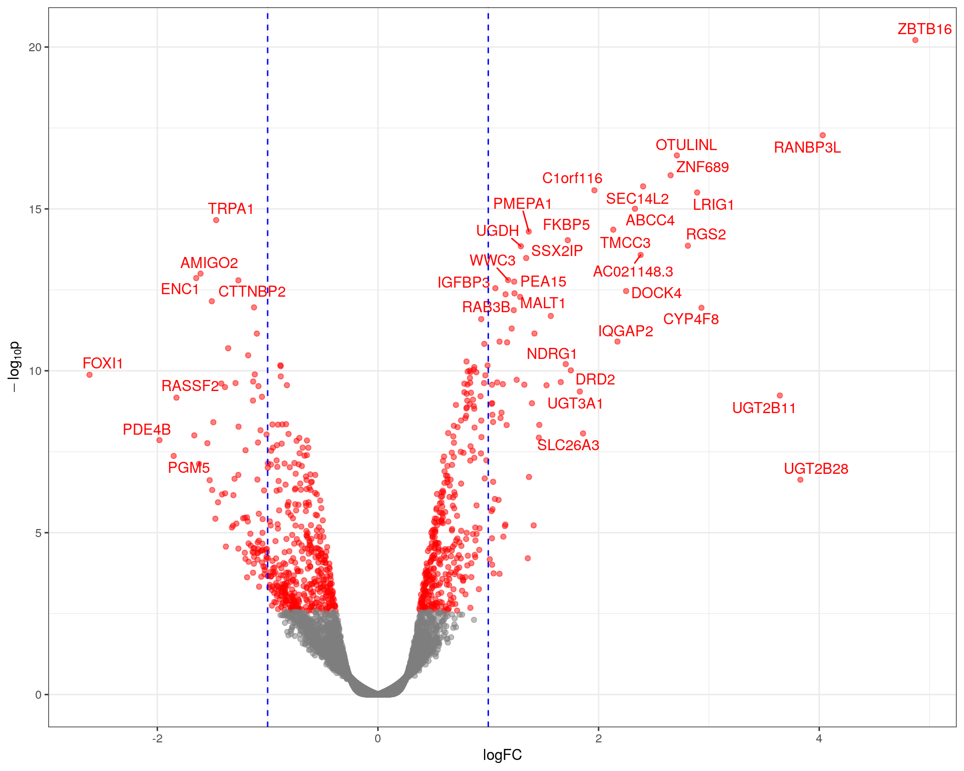
Volcano plot showing significance against log fold-change. The common-use cutoff values for considering a gene as DE (|logFC| > 1) are shown in blue as a guide only as these were not used for this analysis.
Using the sign of logFC to indicate direction, and -\(\log_{10} p\) as the ranking statistic, bias was also checked within the set of results, using GC content and gene length as potential sources of bias amongst the set of DE genes.
_Genes ranked for signed differential expression shown against A) GC Content, and B) Gene Length. Ranks were assigned based on the ranking statistic R = -sign(logFC)*log10p, such that genes at the left are most down-regulated, whilst those at the right are the most up-regulated. Horizontal black lines indicate the overall average value, whilst blue curves indicate the localised GAM fit. A small positive bias was noted at both extremes for both GC content and Gene Length._