Motif Analysis
Steve Pederson
2022-05-25
Last updated: 2022-05-26
Checks: 5 2
Knit directory:
apocrine_signature_mdamb453/
This reproducible R Markdown analysis was created with workflowr (version 1.7.0). The Checks tab describes the reproducibility checks that were applied when the results were created. The Past versions tab lists the development history.
The R Markdown is untracked by Git. To know which version of the R
Markdown file created these results, you’ll want to first commit it to
the Git repo. If you’re still working on the analysis, you can ignore
this warning. When you’re finished, you can run
wflow_publish to commit the R Markdown file and build the
HTML.
Great job! The global environment was empty. Objects defined in the global environment can affect the analysis in your R Markdown file in unknown ways. For reproduciblity it’s best to always run the code in an empty environment.
The command set.seed(20220427) was run prior to running
the code in the R Markdown file. Setting a seed ensures that any results
that rely on randomness, e.g. subsampling or permutations, are
reproducible.
Great job! Recording the operating system, R version, and package versions is critical for reproducibility.
- ame-by-targets
To ensure reproducibility of the results, delete the cache directory
motif_analysis_cache and re-run the analysis. To have
workflowr automatically delete the cache directory prior to building the
file, set delete_cache = TRUE when running
wflow_build() or wflow_publish().
Great job! Using relative paths to the files within your workflowr project makes it easier to run your code on other machines.
Great! You are using Git for version control. Tracking code development and connecting the code version to the results is critical for reproducibility.
The results in this page were generated with repository version 718e311. See the Past versions tab to see a history of the changes made to the R Markdown and HTML files.
Note that you need to be careful to ensure that all relevant files for
the analysis have been committed to Git prior to generating the results
(you can use wflow_publish or
wflow_git_commit). workflowr only checks the R Markdown
file, but you know if there are other scripts or data files that it
depends on. Below is the status of the Git repository when the results
were generated:
Ignored files:
    Ignored:    .Rhistory
    Ignored:    .Rproj.user/
    Ignored:    analysis/motif_analysis_cache/
    Ignored:    data/bigwig/

Untracked files:
    Untracked:  20220523054104_JASPAR2022_combined_matrices_30543_meme.txt
    Untracked:  analysis/motif_analysis.Rmd
    Untracked:  code/check_fimo.R
    Untracked:  code/memes_tutorial.R
    Untracked:  code/seq_comparison.sh
    Untracked:  data/external/HOCOMOCO.v11.meme
    Untracked:  data/external/JASPAR2022_CORE_Hsapiens.meme
    Untracked:  data/external/all4.meme
    Untracked:  output/all4_h3k27ac.fa
    Untracked:  output/all4_no_h3k27ac.fa
    Untracked:  output/ar_foxa1_gata3_no_tfap2b.fa
    Untracked:  output/ar_foxa1_gata3_tfap2b.fa
    Untracked:  output/meme/

Unstaged changes:
    Modified:   analysis/_site.yml
    Modified:   analysis/comparison.Rmd
    Modified:   output/CLCA2.pdf
    Modified:   output/DUSP6.pdf
    Modified:   output/FGFR4.pdf
    Modified:   output/FOXA1.pdf
    Modified:   output/GATA3.pdf
    Modified:   output/GREB1.pdf
    Modified:   output/KYNU.pdf
    Modified:   output/MYB.pdf
    Modified:   output/MYC.pdf
    Modified:   output/PGAP3.pdf
    Modified:   output/TFAP2B.pdf
    Modified:   output/XBP1.pdf
Note that any generated files, e.g. HTML, png, CSS, etc., are not included in this status report because it is ok for generated content to have uncommitted changes.
There are no past versions. Publish this analysis with
wflow_publish() to start tracking its development.
Introduction
This step takes the peaks defined previously and
- Assesses motif enrichment for all ChIP targets within the peaks
- Detect additional binding motifs
As AR is only found bound in the presence of DHT, all peaks are taken using DHT-treatment as the reference condition.
library(memes)
library(universalmotif)
library(tidyverse)
library(plyranges)
library(extraChIPs)
library(rtracklayer)
library(magrittr)
library(BSgenome.Hsapiens.UCSC.hg19)
library(scales)
library(pander)
library(glue)
library(cowplot)
library(parallel)
options(meme_bin = "/opt/meme/bin/")
check_meme_install()
theme_set(theme_bw())
panderOptions("big.mark", ",")stringSetToViews <- function(x) {
stopifnot(is(x, "XStringSet"))
w <- unique(width(x))
stopifnot(length(w) == 1)
n <- length(x)
starts <- (seq_along(x) - 1) * w + 1
seq <- unlist(x)
Views(subject = seq, start = starts, width = w)
}
getBestMatch <- function(x, subject, min.score = "80%", rc = TRUE, ...) {
pwm <- NULL
if (is.matrix(x)) pwm <- x
if (is(x, "universalmotif")) pwm <- x@motif
stopifnot(!is.null(pwm))
stopifnot(is(subject, "XStringViews"))
w <- unique(width(subject))
stopifnot(length(w) == 1)
matches <- matchPWM(
pwm, subject, min.score = min.score, with.score = TRUE, ...
)
df <- as.data.frame(matches)
df$score <- mcols(matches)$score
df$id <- ceiling(df$start/ w)
df$pos <- df$start - (df$id - 1) * w
if (rc) {
rc_matches <- matchPWM(
pwm, subject = reverseComplement(subject),
min.score = min.score, with.score = TRUE,
...
)
rc_df <- as.data.frame(rc_matches)
rc_df$score <- mcols(rc_matches)$score
rc_df$start <- max(end(subject)) - end(rc_matches)
rc_df$end <- max(end(subject)) - start(rc_matches)
rc_df$id <- ceiling(rc_df$start/ w)
rc_df$pos <- rc_df$start - (rc_df$id - 1) * w + 1
df <- bind_rows(df, rc_df)
}
df <- arrange(df, id, desc(score))
df <- distinct(df, id, .keep_all = TRUE)
df <- dplyr::select(df, id, pos, seq)
as_tibble(df)
}hg19 <- BSgenome.Hsapiens.UCSC.hg19
sq19 <- seqinfo(hg19)all_gr <- here::here("data", "annotations", "all_gr.rds") %>%
read_rds() %>%
lapply(
function(x) {
seqinfo(x) <- sq19
x
}
)
counts <- here::here("data", "rnaseq", "counts.out.gz") %>%
read_tsv(skip = 1) %>%
dplyr::select(Geneid, ends_with("bam")) %>%
dplyr::rename(gene_id = Geneid)
detected <- all_gr$gene %>%
as_tibble() %>%
distinct(gene_id, gene_name) %>%
left_join(counts) %>%
pivot_longer(
cols = ends_with("bam"), names_to = "sample", values_to = "counts"
) %>%
mutate(detected = counts > 0) %>%
group_by(gene_id, gene_name) %>%
summarise(detected = mean(detected) > 0.25, .groups = "drop") %>%
dplyr::filter(detected) %>%
dplyr::select(starts_with("gene"))Pre-existing RNA-seq data was again loaded and the set of 21,173 detected genes was defined as those with \(\geq 1\) aligned read in at least 25% of samples. This dataset represented the DHT response in MDA-MB-453 cells, however, given the existence of both Vehicle and DHT conditions, represents a good representative measure of the polyadenylated components of the transcriptome.
features <- here::here("data", "h3k27ac") %>%
  list.files(full.names = TRUE, pattern = "bed$") %>%
  sapply(import.bed, seqinfo = sq19) %>%
  lapply(granges) %>%
  setNames(basename(names(.))) %>%
  setNames(str_remove_all(names(.), "s.bed")) %>%
  GRangesList() %>%
  unlist() %>%
  names_to_column("feature") %>%
  sort()
The set of H3K27ac-defined features was again used as a marker of regulatory activity, with 16,544 and 15,286 regions defined as enhancers or promoters respectively.
meme_db <- here::here("data", "external", "JASPAR2022_CORE_Hsapiens.meme") %>%
  read_meme() %>%
  to_df() %>%
  as_tibble() %>%
  mutate(
    across(everything(), vctrs::vec_proxy),
    altname = str_remove(altname, "MA[0-9]+\\.[0-9]*\\."),
    organism = "Homo sapiens"
  )
meme_db_detected <- meme_db %>%
  mutate(
    gene_name = str_split(altname, pattern = "::", n = 2)
  ) %>%
  dplyr::filter(
    vapply(
      gene_name,
      function(x) all(x %in% detected$gene_name),
      logical(1)
    )
  )
The motif database was initially defined as all 727 CORE motifs found in Homo sapiens, as contained in JASPAR2022. In order to minimise irrelevant results, only the 465 motifs associated with a detected gene were then retained.
dht_peaks <- here::here("data", "peaks") %>%
  list.files(recursive = TRUE, pattern = "oracle", full.names = TRUE) %>%
  sapply(read_rds, simplify = FALSE) %>%
  lapply(function(x) x[["DHT"]]) %>%
  lapply(setNames, nm = c()) %>%
  setNames(str_extract_all(names(.), "AR|FOXA1|GATA3|TFAP2B")) %>%
  lapply(
    function(x) {
      seqinfo(x) <- sq19
      x
    }
  )
targets <- names(dht_peaks)
dht_consensus <- dht_peaks %>%
  lapply(granges) %>%
  GRangesList() %>%
  unlist() %>%
  reduce() %>%
  mutate(
    AR = overlapsAny(., dht_peaks$AR),
    FOXA1 = overlapsAny(., dht_peaks$FOXA1),
    GATA3 = overlapsAny(., dht_peaks$GATA3),
    TFAP2B = overlapsAny(., dht_peaks$TFAP2B),
    promoter = bestOverlap(., features, var = "feature", missing = "None") == "promoter",
    enhancer = bestOverlap(., features, var = "feature", missing = "None") == "enhancer",
    H3K27ac = promoter | enhancer
  )
a <- dht_peaks %>%
lapply(mutate, w = width) %>%
lapply(as_tibble) %>%
bind_rows(.id = "target") %>%
ggplot(aes(w, stat(density), colour = target)) +
geom_density() +
scale_x_log10(breaks = c(100, 300, 600, 1e3, 2e3, 3e3), labels = comma) +
labs(
x = "Peak Width (bp)", y = "Density", colour = "Target"
)
b <- dht_peaks %>%
lapply(mutate, w = width) %>%
lapply(as_tibble) %>%
bind_rows(.id = "target") %>%
mutate(skew = 0.5 - peak / w) %>%
ggplot(aes(skew, stat(density), colour = target)) +
geom_density() +
scale_x_continuous(labels = percent) +
labs(
x = "% Width Between Peak Summit and Peak Centre",
y = "Density",
colour = "ChIP Target"
)
plot_grid(
a + theme(legend.position = "none"),
b + theme(legend.position = "none"),
get_legend(b),
rel_widths = c(1, 1, 0.2), nrow = 1,
labels = c("A", "B")
)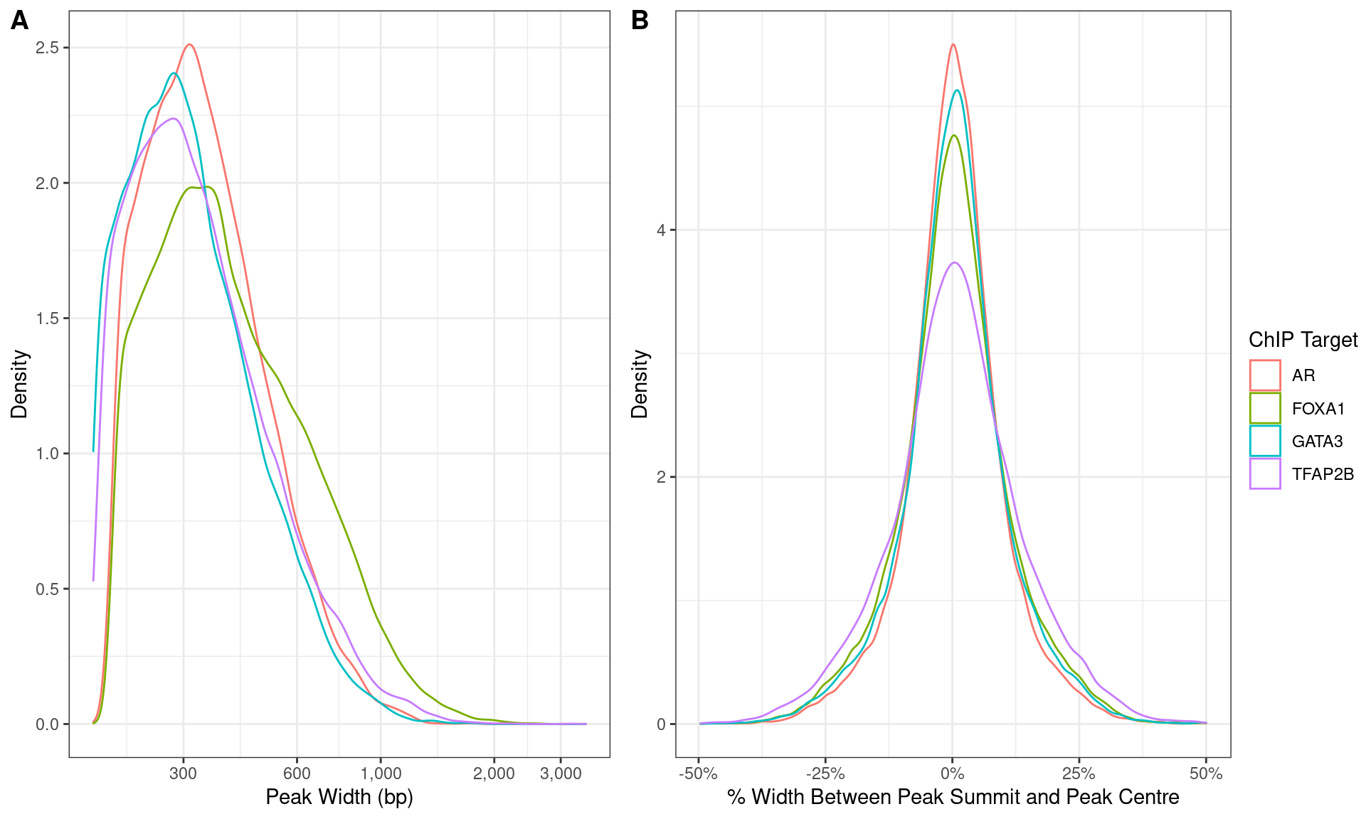
Distributions of A) peak width and B) summit location with peaks.
Enrichment of Expected Motifs
Analysis of Motif Enrichment (AME)
grl_by_targets <- dht_consensus %>%
  as_tibble() %>%
  pivot_longer(
    all_of(targets), names_to = "target", values_to = "detected"
  ) %>%
  dplyr::filter(detected) %>%
  group_by(range, H3K27ac) %>%
  summarise(
    targets = paste(sort(target), collapse = " "),
    .groups = "drop"
  ) %>%
  colToRanges(var = "range", seqinfo = sq19) %>%
  sort() %>%
  splitAsList(.$targets)
Union ranges were grouped by the combination of detected AR, FOXA1, GATA3 and TFAP2B binding, then sequences obtained corresponding to each union range.
grl_by_targets %>%
  lapply(
    function(x) {
      tibble(
        `N Sites` = length(x),
        `% H3K27ac` = mean(x$H3K27ac),
        `Median Width` = floor(median(width(x)))
      )
    }
  ) %>%
  bind_rows(.id = "Targets") %>%
  mutate(
    `N Targets` = str_count(Targets, " ") + 1,
    `% H3K27ac` = percent(`% H3K27ac`, 0.1)
  ) %>%
  dplyr::select(contains("Targets"), everything()) %>%
  arrange(`N Targets`, Targets) %>%
  pander(
    justify = "lrrrr",
    caption = "Summary of union ranges and which combinations of the targets were detected."
)| Targets | N Targets | N Sites | % H3K27ac | Median Width |
|---|---|---|---|---|
| AR | 1 | 395 | 13.9% | 241 |
| FOXA1 | 1 | 59,404 | 12.8% | 319 |
| GATA3 | 1 | 4,284 | 19.6% | 234 |
| TFAP2B | 1 | 6,655 | 80.1% | 301 |
| AR FOXA1 | 2 | 3,543 | 17.8% | 505 |
| AR GATA3 | 2 | 158 | 16.5% | 310 |
| AR TFAP2B | 2 | 135 | 55.6% | 414 |
| FOXA1 GATA3 | 2 | 9,760 | 18.1% | 479 |
| FOXA1 TFAP2B | 2 | 3,849 | 64.6% | 513 |
| GATA3 TFAP2B | 2 | 396 | 60.6% | 368 |
| AR FOXA1 GATA3 | 3 | 6,518 | 25.2% | 683 |
| AR FOXA1 TFAP2B | 3 | 1,786 | 62.9% | 639 |
| AR GATA3 TFAP2B | 3 | 61 | 55.7% | 419 |
| FOXA1 GATA3 TFAP2B | 3 | 1,441 | 52.0% | 575 |
| AR FOXA1 GATA3 TFAP2B | 4 | 6,336 | 58.2% | 814 |
meme_db_targets <- meme_db_detected %>%
  dplyr::filter(altname %in% targets) %>%
  to_list()
seq_by_targets <- grl_by_targets %>%
  get_sequence(hg19)
ame_by_targets <- seq_by_targets %>%
  runAme(database = meme_db_targets)
AME from the meme-suite was then run on each sequence to detect the presence of motifs associated with each target within each set of sequences.
ame_by_targets %>%
  bind_rows(.id = "targets") %>%
  mutate(
    motif_id = as.factor(motif_id),
    targets = as.factor(targets),
    TFAP2B = ifelse(
      str_detect(targets, "TFAP2B"), "TFAP2B", "No TFAP2B"
    )
  ) %>%
  dplyr::filter(adj.pvalue < 0.05) %>%
  plot_ame_heatmap(
    id = motif_id,
    value = tp_percent,
    group = targets
  ) +
  geom_label(
    aes(label = percent(tp_percent/100, 0.1)),
    size = 3,
    show.legend = FALSE
  ) +
  facet_grid(TFAP2B ~ motif_alt_id, scales = "free", space = "free") +
  scale_x_discrete(expand = expansion(c(0, 0))) +
  scale_y_discrete(expand = expansion(c(0, 0))) +
  labs(
    x = "Detected Motif",
    y = "Detected Targets",
    fill = expression(widehat("TP%"))
  ) +
  theme(
    axis.text.x = element_text(angle = 0, hjust = 0.5, size = 10),
    axis.text.y = element_text(angle = 0, hjust = 1, size = 10),
    panel.grid = element_blank()
  )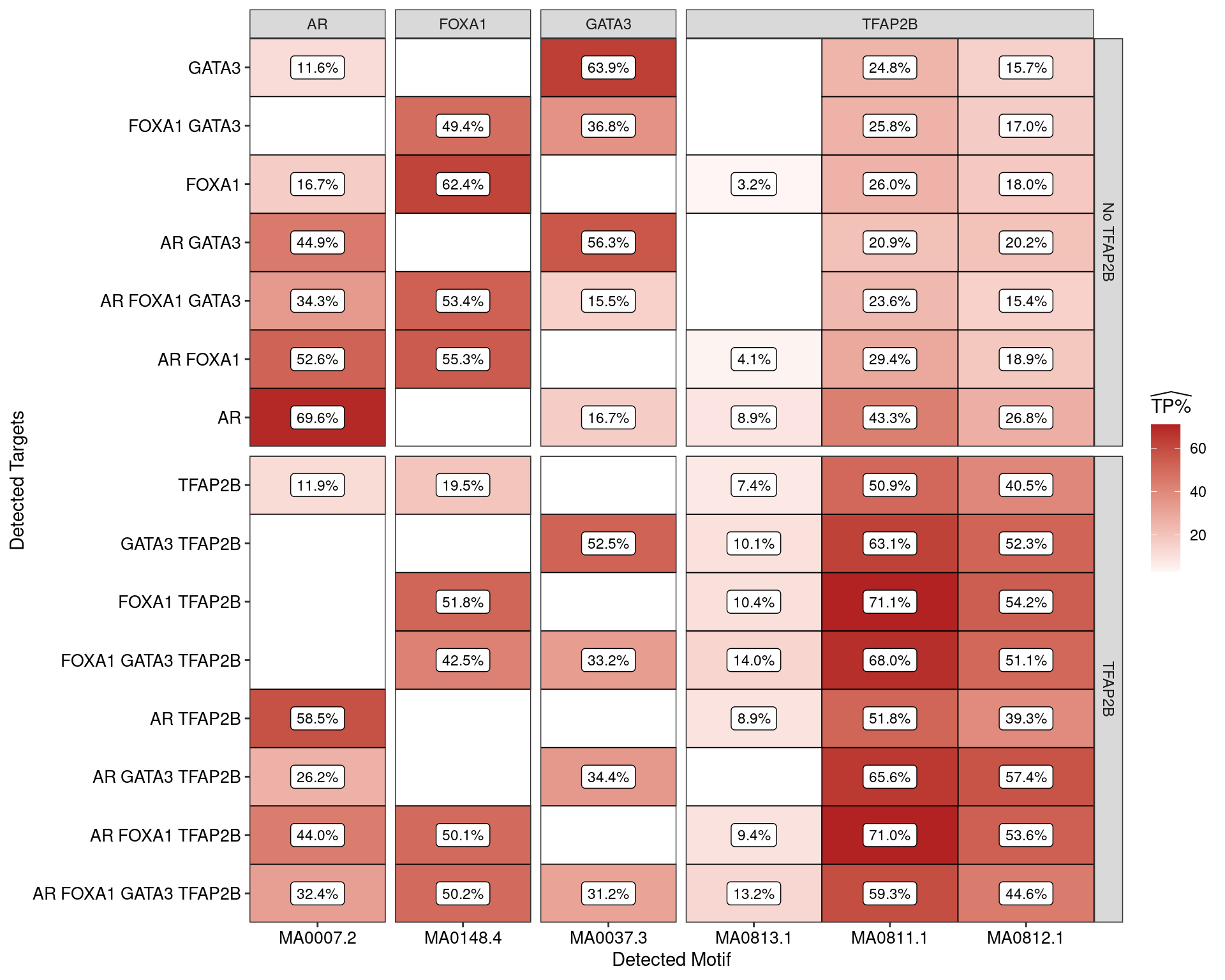
Estimated percentage of true positive matches to all binding motifs associated with each ChIP target. Only values with an enrichment adjusted p-value < 0.05 are shown, such that missing values are able to be confidently assumed as not enriched for the motif. With the possible exception of GATA3 binding in the presence of AR and FOXA1 only, all provide supporting evidence for direct binding of each target to it’s motif
Motif Centrality Relative to TFAP2B
seq_width <- 200
min_score <- percent(0.75, accuracy = 1)
tfap2b_summits <- dht_peaks$TFAP2B %>%
  resize(width = 1, fix = 'start') %>%
  shift(shift = .$peak) %>%
  resize(width = seq_width, fix = 'center') %>%
  granges() %>%
  mutate(
    AR = overlapsAny(., subset(dht_consensus, AR)),
    FOXA1 = overlapsAny(., subset(dht_consensus, FOXA1)),
    GATA3 = overlapsAny(., subset(dht_consensus, GATA3)),
    H3K27ac = overlapsAny(., features)
  )
seq_tfap2b_summits <- tfap2b_summits %>%
  get_sequence(hg19)
views_tfap2b_summits <- stringSetToViews(seq_tfap2b_summits)
matches_tfap2b_summits <- meme_db_targets %>%
  lapply(
    getBestMatch,
    subject = views_tfap2b_summits,
    min.score = min_score
  ) %>%
  setNames(
    vapply(meme_db_targets, function(x) x@name, character(1))
  ) %>%
  bind_rows(.id = "name") %>%
  left_join(
    dplyr::select(meme_db_detected, name, altname),
    by = "name"
  ) %>%
  left_join(
    tfap2b_summits %>%
      as_tibble() %>%
      mutate(id =seq_along(range)),
    by = "id"
  ) %>%
  arrange(id) %>%
  dplyr::select(range, any_of(targets), H3K27ac, name, altname, seq, pos)
Using the sites which only show detectable TFAP2B, the central 200bp region around the estimated TFAP2B peak summit were then assessed for binding of each of the motifs associated with the set of ChIP targets. Any matches with a match greater than 75% of the highest possible score were initially included, with the position of only the best scoring match being retained. The position of the best match, relative to the peak centre was then assessed.
matches_tfap2b_summits  %>%
  mutate(name = glue("{name}\n({altname})")) %>%
  ggplot(aes(pos, stat(density), colour = altname)) +
  geom_density(aes(linetype = H3K27ac)) +
  geom_text(
    aes(x = seq_width/2, y = 0.001, label = lab),
    data = . %>%
      group_by(name) %>%
      summarise(
        n = dplyr::n(), .groups = "drop") %>%
      mutate(lab = glue("n = {comma(n)}\n({percent(n/length(tfap2b_summits), 0.1)})")),
    colour = "black",
    inherit.aes = FALSE
  ) +
  facet_wrap(~name) +
  scale_linetype_manual(values = c(2, 1)) +
  labs(
    x = "Best Match Position In Sequence",
    y = "Density",
    colour = "Motif Target"
  )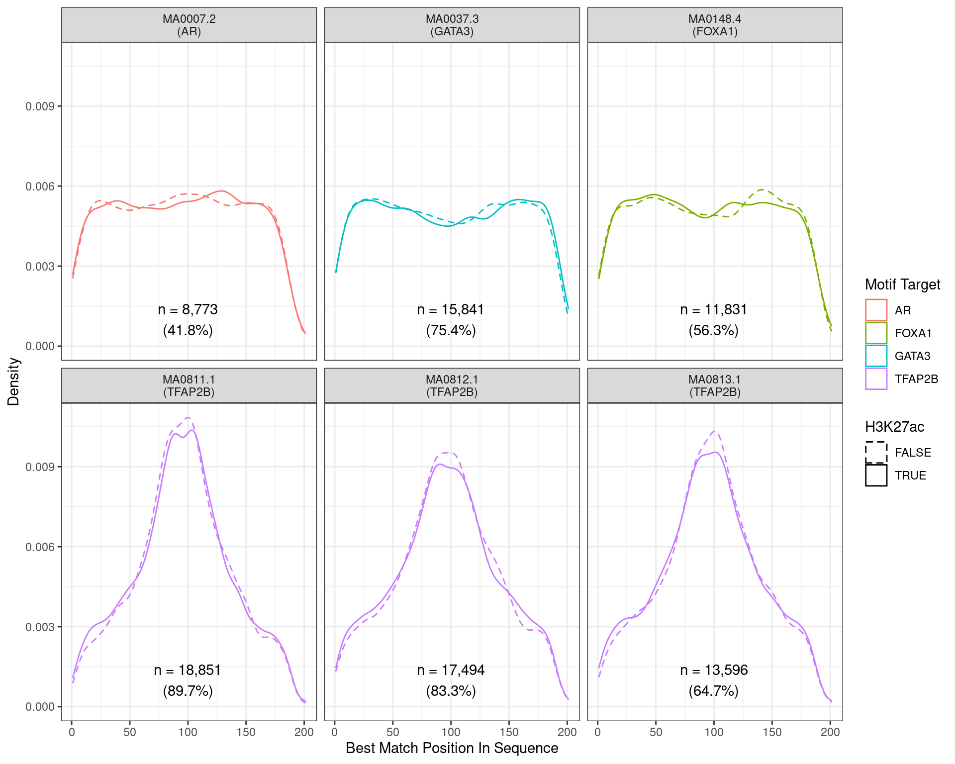
Position of the best match for each motif using sequences centred at the summits of TFAP2B binding sites. Sites where H3K27ac signal was not found are shown as dashed lines. No visual difference in TFAP2B motif centrality was detected. All other motifs appeared to be uniformly distributed amongst the sequences.
Across all motifs which were considered to represent possible matches to the binding site of TFAP2\(\beta\), matches to one or more of the motifs were found in 20,382 (97.0%) of the 21,008 queried sequences.
Motif Discovery
sessionInfo()R version 4.2.0 (2022-04-22)
Platform: x86_64-pc-linux-gnu (64-bit)
Running under: Ubuntu 20.04.4 LTS
Matrix products: default
BLAS: /usr/lib/x86_64-linux-gnu/blas/libblas.so.3.9.0
LAPACK: /usr/lib/x86_64-linux-gnu/lapack/liblapack.so.3.9.0
locale:
[1] LC_CTYPE=en_AU.UTF-8 LC_NUMERIC=C
[3] LC_TIME=en_AU.UTF-8 LC_COLLATE=en_AU.UTF-8
[5] LC_MONETARY=en_AU.UTF-8 LC_MESSAGES=en_AU.UTF-8
[7] LC_PAPER=en_AU.UTF-8 LC_NAME=C
[9] LC_ADDRESS=C LC_TELEPHONE=C
[11] LC_MEASUREMENT=en_AU.UTF-8 LC_IDENTIFICATION=C
attached base packages:
[1] parallel stats4 stats graphics grDevices utils datasets
[8] methods base
other attached packages:
[1] cowplot_1.1.1 glue_1.6.2
[3] pander_0.6.5 scales_1.2.0
[5] BSgenome.Hsapiens.UCSC.hg19_1.4.3 BSgenome_1.64.0
[7] Biostrings_2.64.0 XVector_0.36.0
[9] magrittr_2.0.3 rtracklayer_1.56.0
[11] extraChIPs_1.0.0 SummarizedExperiment_1.26.1
[13] Biobase_2.56.0 MatrixGenerics_1.8.0
[15] matrixStats_0.62.0 BiocParallel_1.30.2
[17] plyranges_1.16.0 GenomicRanges_1.48.0
[19] GenomeInfoDb_1.32.2 IRanges_2.30.0
[21] S4Vectors_0.34.0 BiocGenerics_0.42.0
[23] forcats_0.5.1 stringr_1.4.0
[25] dplyr_1.0.9 purrr_0.3.4
[27] readr_2.1.2 tidyr_1.2.0
[29] tibble_3.1.7 ggplot2_3.3.6
[31] tidyverse_1.3.1 universalmotif_1.14.0
[33] memes_1.4.1 workflowr_1.7.0
loaded via a namespace (and not attached):
[1] utf8_1.2.2 R.utils_2.11.0
[3] tidyselect_1.1.2 RSQLite_2.2.14
[5] AnnotationDbi_1.58.0 htmlwidgets_1.5.4
[7] grid_4.2.0 scatterpie_0.1.7
[9] munsell_0.5.0 codetools_0.2-18
[11] withr_2.5.0 colorspace_2.0-3
[13] filelock_1.0.2 highr_0.9
[15] knitr_1.39 rstudioapi_0.13
[17] ggside_0.2.0.9990 labeling_0.4.2
[19] git2r_0.30.1 GenomeInfoDbData_1.2.8
[21] polyclip_1.10-0 farver_2.1.0
[23] bit64_4.0.5 rprojroot_2.0.3
[25] vctrs_0.4.1 generics_0.1.2
[27] xfun_0.31 csaw_1.30.1
[29] biovizBase_1.44.0 BiocFileCache_2.4.0
[31] ggseqlogo_0.1 R6_2.5.1
[33] doParallel_1.0.17 clue_0.3-60
[35] locfit_1.5-9.5 AnnotationFilter_1.20.0
[37] bitops_1.0-7 cachem_1.0.6
[39] DelayedArray_0.22.0 assertthat_0.2.1
[41] vroom_1.5.7 promises_1.2.0.1
[43] BiocIO_1.6.0 nnet_7.3-17
[45] gtable_0.3.0 processx_3.5.3
[47] ensembldb_2.20.1 rlang_1.0.2
[49] GlobalOptions_0.1.2 splines_4.2.0
[51] lazyeval_0.2.2 dichromat_2.0-0.1
[53] broom_0.8.0 checkmate_2.1.0
[55] yaml_2.3.5 modelr_0.1.8
[57] GenomicFeatures_1.48.1 backports_1.4.1
[59] httpuv_1.6.5 Hmisc_4.7-0
[61] EnrichedHeatmap_1.26.0 usethis_2.1.5
[63] tools_4.2.0 ellipsis_0.3.2
[65] jquerylib_0.1.4 RColorBrewer_1.1-3
[67] Rcpp_1.0.8.3 base64enc_0.1-3
[69] progress_1.2.2 zlibbioc_1.42.0
[71] RCurl_1.98-1.6 ps_1.7.0
[73] prettyunits_1.1.1 rpart_4.1.16
[75] GetoptLong_1.0.5 ggrepel_0.9.1
[77] haven_2.5.0 cluster_2.1.3
[79] here_1.0.1 fs_1.5.2
[81] data.table_1.14.2 circlize_0.4.15
[83] reprex_2.0.1 whisker_0.4
[85] ProtGenerics_1.28.0 pkgload_1.2.4
[87] hms_1.1.1 evaluate_0.15
[89] XML_3.99-0.9 jpeg_0.1-9
[91] readxl_1.4.0 gridExtra_2.3
[93] shape_1.4.6 testthat_3.1.4
[95] compiler_4.2.0 biomaRt_2.52.0
[97] crayon_1.5.1 R.oo_1.24.0
[99] htmltools_0.5.2 ggfun_0.0.6
[101] later_1.3.0 tzdb_0.3.0
[103] Formula_1.2-4 lubridate_1.8.0
[105] DBI_1.1.2 tweenr_1.0.2
[107] dbplyr_2.1.1 ComplexHeatmap_2.12.0
[109] MASS_7.3-56 GenomicInteractions_1.30.0
[111] rappdirs_0.3.3 Matrix_1.4-1
[113] brio_1.1.3 cli_3.3.0
[115] R.methodsS3_1.8.1 metapod_1.4.0
[117] Gviz_1.40.1 igraph_1.3.1
[119] pkgconfig_2.0.3 getPass_0.2-2
[121] GenomicAlignments_1.32.0 foreign_0.8-82
[123] xml2_1.3.3 InteractionSet_1.24.0
[125] foreach_1.5.2 bslib_0.3.1
[127] rvest_1.0.2 VariantAnnotation_1.42.1
[129] callr_3.7.0 digest_0.6.29
[131] rmarkdown_2.14 cellranger_1.1.0
[133] htmlTable_2.4.0 edgeR_3.38.1
[135] restfulr_0.0.13 curl_4.3.2
[137] Rsamtools_2.12.0 rjson_0.2.21
[139] lifecycle_1.0.1 jsonlite_1.8.0
[141] desc_1.4.1 limma_3.52.1
[143] fansi_1.0.3 pillar_1.7.0
[145] lattice_0.20-45 KEGGREST_1.36.0
[147] fastmap_1.1.0 httr_1.4.3
[149] survival_3.2-13 png_0.1-7
[151] iterators_1.0.14 cmdfun_1.0.2
[153] bit_4.0.4 ggforce_0.3.3
[155] stringi_1.7.6 sass_0.4.1
[157] blob_1.2.3 latticeExtra_0.6-29
[159] memoise_2.0.1