Comparison of all ChIP Targets
Stephen Pederson
20 May, 2022
Last updated: 2022-05-20
Checks: 6 1
Knit directory:
apocrine_signature_mdamb453/
This reproducible R Markdown analysis was created with workflowr (version 1.7.0). The Checks tab describes the reproducibility checks that were applied when the results were created. The Past versions tab lists the development history.
The R Markdown file has unstaged changes. To know which version of
the R Markdown file created these results, you’ll want to first commit
it to the Git repo. If you’re still working on the analysis, you can
ignore this warning. When you’re finished, you can run
wflow_publish to commit the R Markdown file and build the
HTML.
Great job! The global environment was empty. Objects defined in the global environment can affect the analysis in your R Markdown file in unknown ways. For reproduciblity it’s best to always run the code in an empty environment.
The command set.seed(20220427) was run prior to running
the code in the R Markdown file. Setting a seed ensures that any results
that rely on randomness, e.g. subsampling or permutations, are
reproducible.
Great job! Recording the operating system, R version, and package versions is critical for reproducibility.
Nice! There were no cached chunks for this analysis, so you can be confident that you successfully produced the results during this run.
Great job! Using relative paths to the files within your workflowr project makes it easier to run your code on other machines.
Great! You are using Git for version control. Tracking code development and connecting the code version to the results is critical for reproducibility.
The results in this page were generated with repository version 5597186. See the Past versions tab to see a history of the changes made to the R Markdown and HTML files.
Note that you need to be careful to ensure that all relevant files for
the analysis have been committed to Git prior to generating the results
(you can use wflow_publish or
wflow_git_commit). workflowr only checks the R Markdown
file, but you know if there are other scripts or data files that it
depends on. Below is the status of the Git repository when the results
were generated:
Ignored files:
    Ignored:    .Rhistory
    Ignored:    .Rproj.user/
    Ignored:    data/bigwig/

Unstaged changes:
    Modified:   analysis/comparison.Rmd
    Modified:   output/MYC.pdf
Note that any generated files, e.g. HTML, png, CSS, etc., are not included in this status report because it is ok for generated content to have uncommitted changes.
These are the previous versions of the repository in which changes were
made to the R Markdown (analysis/comparison.Rmd) and HTML
(docs/comparison.html) files. If you’ve configured a remote
Git repository (see ?wflow_git_remote), click on the
hyperlinks in the table below to view the files as they were in that
past version.
| File | Version | Author | Date | Message |
|---|---|---|---|---|
| Rmd | 5597186 | Steve Pederson | 2022-05-19 | Added MYC plot |
| Rmd | 1ba686b | Steve Pederson | 2022-05-19 | EOD Wed |
| Rmd | e742af3 | Steve Pederson | 2022-05-16 | Started exploring mapped genes |
| html | e742af3 | Steve Pederson | 2022-05-16 | Started exploring mapped genes |
| Rmd | 792bb98 | Steve Pederson | 2022-05-13 | Added dist to TSS |
| html | 792bb98 | Steve Pederson | 2022-05-13 | Added dist to TSS |
| Rmd | e9956d4 | Steve Pederson | 2022-05-13 | Added 95% CIs for targets |
| html | e9956d4 | Steve Pederson | 2022-05-13 | Added 95% CIs for targets |
| Rmd | 1582607 | Steve Pederson | 2022-05-12 | Started looking at H3K27ac |
| Rmd | 8217e8a | Steve Pederson | 2022-05-10 | Started explorations |
| html | 8217e8a | Steve Pederson | 2022-05-10 | Started explorations |
Introduction
library(tidyverse)
library(magrittr)
library(extraChIPs)
library(plyranges)
library(pander)
library(scales)
library(reactable)
library(htmltools)
library(UpSetR)
library(rtracklayer)
library(GenomicInteractions)
library(multcomp)
library(glue)
library(nnet)
library(effects)
library(Gviz)
library(readxl)
library(corrplot)
library(goseq)
theme_set(theme_bw())
bar_chart <- function(label, width = "100%", height = "16px", fill = "#00bfc4", background = NULL) {
bar <- div(style = list(background = fill, width = width, height = height))
chart <- div(style = list(flexGrow = 1, marginLeft = "8px", background = background), bar)
div(style = list(display = "flex", alignItems = "center"), label, chart)
}
bar_style <- function(width = 1, fill = "#e6e6e6", height = "75%", align = c("left", "right"), color = NULL) {
align <- match.arg(align)
if (align == "left") {
position <- paste0(width * 100, "%")
image <- sprintf("linear-gradient(90deg, %1$s %2$s, transparent %2$s)", fill, position)
} else {
position <- paste0(100 - width * 100, "%")
image <- sprintf("linear-gradient(90deg, transparent %1$s, %2$s %1$s)", position, fill)
}
list(
backgroundImage = image,
backgroundSize = paste("100%", height),
backgroundRepeat = "no-repeat",
backgroundPosition = "center",
color = color
)
}dht_peaks <- here::here("data", "peaks") %>%
list.files(recursive = TRUE, pattern = "oracle", full.names = TRUE) %>%
sapply(read_rds, simplify = FALSE) %>%
lapply(function(x) x[["DHT"]]) %>%
lapply(setNames, nm = c()) %>%
setNames(str_extract_all(names(.), "AR|FOXA1|GATA3|TFAP2B"))
dht_consensus <- dht_peaks %>%
lapply(granges) %>%
GRangesList() %>%
unlist() %>%
reduce() %>%
mutate(
AR = overlapsAny(., dht_peaks$AR),
FOXA1 = overlapsAny(., dht_peaks$FOXA1),
GATA3 = overlapsAny(., dht_peaks$GATA3),
TFAP2B = overlapsAny(., dht_peaks$TFAP2B),
)
targets <- names(dht_peaks)
sq <- seqinfo(dht_consensus)Relationship Between Binding Regions
Oracle peaks from the DHT-treated samples in each ChIP target were obtained previously using the GRAVI workflow. AR and GATA3 peaks were derived from the same samples/passages, whilst FOXA1 and TFAP2B ChIP-Seq experiments were performed separately.
cp <- htmltools::tags$em(
  "Summary of all oracle peaks from DHT-treated samples. FOXA1 clearly showed the most binding activity."
)
tbl <- dht_peaks %>%
  lapply(
    function(x) {
      tibble(
        n = length(x),
        w = median(width(x)),
        kb = sum(width(x)) / 1e3
      )
    }
  ) %>%
  lapply(list) %>%
  as_tibble() %>%
  pivot_longer(cols = everything(), names_to = "target") %>%
  unnest(everything()) %>%
  reactable(
    filterable = FALSE, searchable = FALSE,
    columns = list(
      target = colDef(name = "ChIP Target"),
      n = colDef(name = "Total Peaks"),
      w = colDef(name = "Median Width"),
      kb = colDef(name = "Total Width (kb)", format = colFormat(digits = 1))
    ),
    defaultColDef = colDef(
      format = colFormat(separators = TRUE, digits = 0)
    )
  )
div(class = "table",
  div(class = "table-header",
      div(class = "caption", cp),
      tbl
  )
)A set of target-agnostic set of binding regions was then defined as the union of all DHT-treat peaks across all targets.
dht_consensus %>%
  as_tibble() %>%
  pivot_longer(cols = all_of(targets), names_to = "target", values_to = "bound") %>%
  dplyr::filter(bound) %>%
  split(.$target) %>%
  lapply(pull, "range") %>%
  fromList() %>%
  upset(
    sets = rev(targets), keep.order = TRUE,
    order.by = "freq",
    set_size.show = TRUE, set_size.scale_max = nrow(.)
  )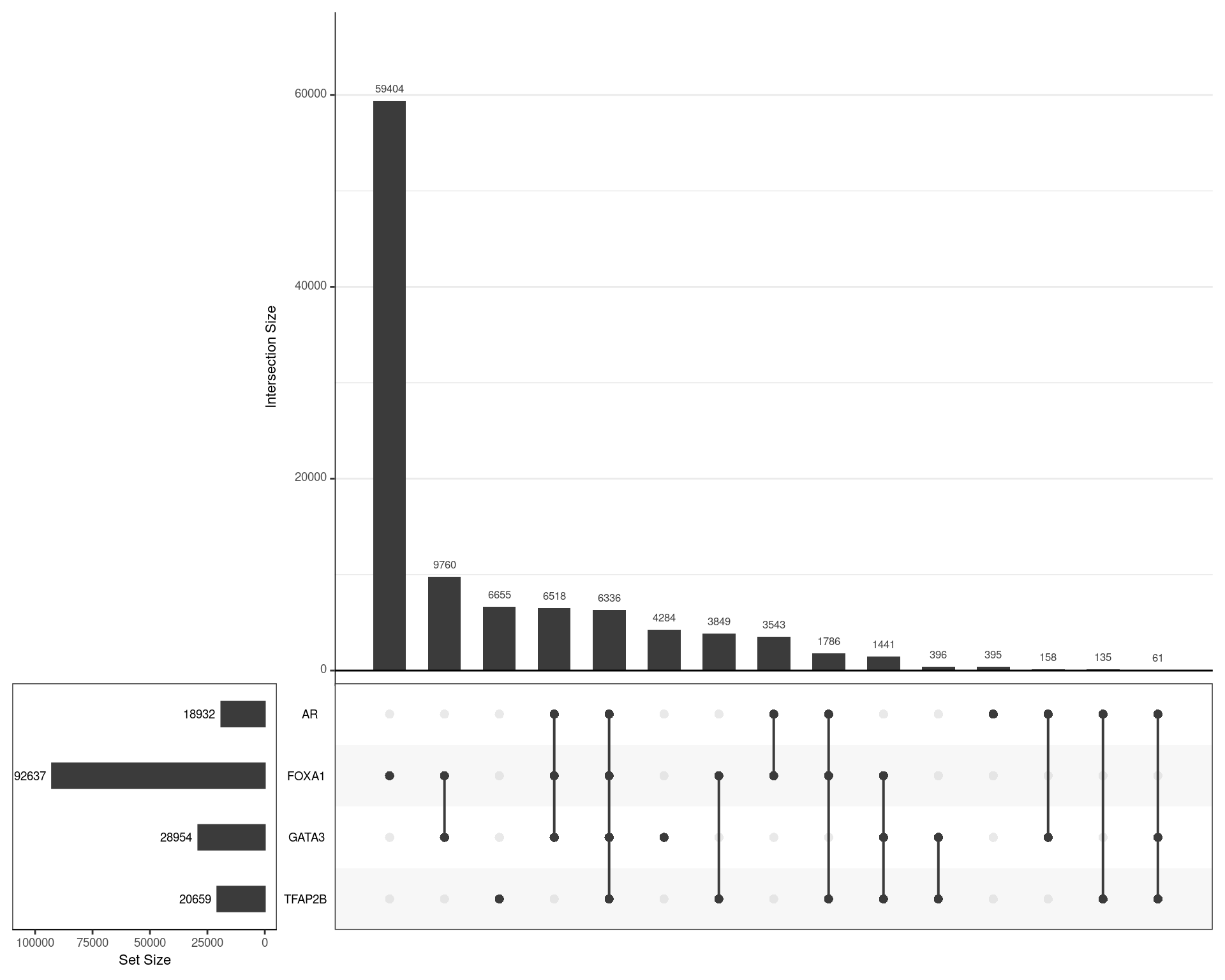
Using the union of all binding regions, those which overlapped an oracle peak from each ChIP target are shown
H3K27ac Signal
Given the hypothesis that the co-ocurrence of all 4 ChIP targets should be associated with increased transcriptional or regulatory activity, the set of all DHT peaks were then compared to promoters and enhancers derived H2K27ac binding, as detected in the existing GATA3/AR dataset produced by Leila Hosseinzadeh. Any H3K27ac peak detected in this dataset was classified either as a promoter or enhancer, and thus these features can be considered as the complete set of regions with detectable H3K27ac signal from this experiment.
all_gr <- here::here("data", "annotations", "all_gr.rds") %>%
  read_rds()
tss <- resize(all_gr$transcript, width = 1)
features <- here::here("data", "h3k27ac") %>%
  list.files(full.names = TRUE, pattern = "bed$") %>%
  sapply(import.bed, seqinfo = sq) %>%
  lapply(granges) %>%
  setNames(basename(names(.))) %>%
  setNames(str_remove_all(names(.), "s.bed")) %>%
  GRangesList() %>%
  unlist() %>%
  names_to_column("feature") %>%
  sort()
dht_consensus %<>%
  mutate(
    promoter = bestOverlap(., features, var = "feature", missing = "None") == "promoter",
    enhancer = bestOverlap(., features, var = "feature", missing = "None") == "enhancer",
    H3K27ac = promoter | enhancer,
    dist_to_tss = mcols(distanceToNearest(., tss, ignore.strand = TRUE))$distance
  )
fs <- 12
cp <- htmltools::tags$em(
glue(
"Summary of all sites, taking the union of all sites with any target bound. ",
"{comma(length(dht_consensus))} sites were found across all targets. ",
"Individual ChIP targets can be searched within this table using 't' or 'f' ",
"to denote True or False. Summaries regarding association with H3K27ac ",
"peaks and distance to the nearest TSS are also provided. ",
"The total numbers of sites overlapping H3K27ac-defined Promoters and ",
"Enhancers are shown with the % of sites being relative to to those ",
"overlapping H3K27ac-defined features"
)
)
tbl <- dht_consensus %>%
as_tibble() %>%
group_by(!!!syms(targets)) %>%
summarise(
n = dplyr::n(),
nH3K27ac = sum(H3K27ac),
H3K27ac = mean(H3K27ac),
promoter = sum(promoter),
enhancer = sum(enhancer),
d = median(dist_to_tss),
.groups = "drop"
) %>%
arrange(desc(n)) %>%
reactable(
filterable = TRUE,
pagination = FALSE,
columns = list(
AR = colDef(
cell = function(value) {
ifelse(value, "\u2714", "\u2716")
},
style = function(value) {
cl <- ifelse(value, "forestgreen", "red")
list(color = cl)
},
maxWidth = 60
),
FOXA1 = colDef(
cell = function(value) {
ifelse(value, "\u2714", "\u2716")
},
style = function(value) {
cl <- ifelse(value, "forestgreen", "red")
list(color = cl)
},
maxWidth = 60
),
GATA3 = colDef(
cell = function(value) {
ifelse(value, "\u2714", "\u2716")
},
style = function(value) {
cl <- ifelse(value, "forestgreen", "red")
list(color = cl)
},
maxWidth = 60
),
TFAP2B = colDef(
cell = function(value) {
ifelse(value, "\u2714", "\u2716")
},
style = function(value) {
cl <- ifelse(value, "forestgreen", "red")
list(color = cl)
},
maxWidth = 70
),
n = colDef(
name = "Nbr. Sites",
format = colFormat(separators = TRUE),
maxWidth = 75
),
nH3K27ac = colDef(
name = "Overlapping H3K27ac",
format = colFormat(separators = TRUE),
maxWidth = 85
),
H3K27ac = colDef(
name = "% H3K27ac Overlap",
format = colFormat(digits = 1, percent = TRUE),
style = function(value) {
bar_style(width = value, align = "right")
},
maxWidth = 80
),
promoter = colDef(
name = "Promoters",
style = function(value, index) {
bar_style(
width = 0.5*(value / .$nH3K27ac[[index]]), align = "right",
fill = rgb(1, 0.416, 0.416)
)
},
cell = function(value, index) {
lb <- glue("{value} ({percent(value / .$nH3K27ac[[index]], 1)})")
as.character(lb)
},
align = "left",
minWidth = 120
),
enhancer = colDef(
name = "Enhancers",
style = function(value, index) {
bar_style(
width = 0.5*(value / .$nH3K27ac[[index]]), align = "left",
fill = rgb(1, 0.65, 0.2)
)
},
cell = function(value, index) {
lb <- glue("{value} ({percent(value / .$nH3K27ac[[index]], 1)})")
as.character(lb)
},
align = "right",
minWidth = 120
),
d = colDef(
name = "Median Distance to TSS (bp)",
format = colFormat(digits = 0, separators = TRUE)
)
),
style = list(fontSize = fs)
)
div(class = "table",
div(class = "table-header",
div(class = "caption", cp),
tbl
)
)All H3K27ac Peaks
grp_h3k27ac <- dht_consensus %>%
  as_tibble() %>%
  dplyr::select(range, all_of(targets), H3K27ac) %>%
  pivot_longer(cols = all_of(targets), names_to = "targets") %>%
  dplyr::filter(value) %>%
  group_by(range, H3K27ac) %>%
  summarise(targets = paste(targets, collapse = "+"), .groups = "drop")
glm_h3k27ac <- glm(H3K27ac ~ 0 + targets, family = "binomial", data = grp_h3k27ac)
A simple logistic regression model was then run to estimate the probability of overlapping a peak associated with the histone mark H3K27ac for each combination of ChIP targets. Binding of TFAP2\(\beta\) in isolation clearly had the strongest association with H3K27ac peaks, whilst the absence of TFAP2\(\beta\) clearly reduced the likelihood of all other ChIP targets being associated with H3K27ac signal.
inv.logit <- binomial()$linkinv
glm_h3k27ac %>%
  glht() %>%
  confint() %>%
  .[["confint"]] %>%
  as_tibble(rownames = "targets") %>%
  mutate(
    n_targets = str_count(targets, "\\+") + 1
  ) %>%
  arrange(desc(n_targets), desc(targets)) %>%
  mutate(
    targets = fct_inorder(targets) %>%
      fct_relabel(str_remove_all, pattern = "targets"),
    p = inv.logit(Estimate),
    TFAP2B = ifelse(str_detect(targets, "TFAP2B"), "TFAP2B", "No TFAP2B"),
    across(all_of(c("upr", "lwr")), inv.logit)
  ) %>%
  ggplot(aes(p, targets)) +
  geom_point() +
  geom_errorbarh(aes(xmin = lwr, xmax = upr), height = 0.4, colour = "grey20") +
  facet_grid(TFAP2B ~ ., scales = "free_y") +
  scale_x_continuous(limits = c(0, 1)) +
  labs(x = "Probability of H3K27ac Peak Overlap", y = "Detected Targets")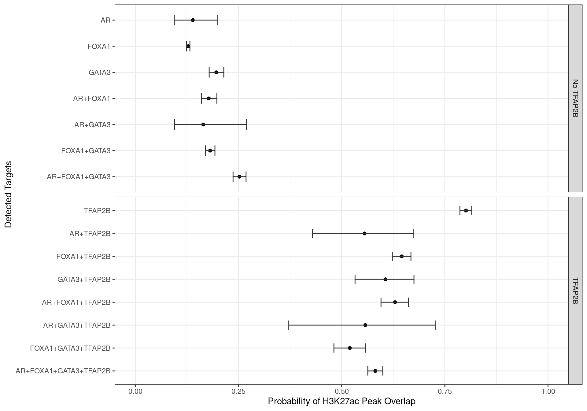
Family-wise 95% Confidence Intervals for the probability of overlapping an H3K27ac-derived feature, based on the combinations of detected ChIP targets.
Promoters Only
grp_prom <- dht_consensus %>%
  as_tibble() %>%
  dplyr::select(range, all_of(targets), promoter) %>%
  pivot_longer(cols = all_of(targets), names_to = "targets") %>%
  dplyr::filter(value) %>%
  group_by(range, promoter) %>%
  summarise(targets = paste(targets, collapse = "+"), .groups = "drop")
glm_prom <- glm(promoter ~ 0 + targets, family = "binomial", data = grp_prom)
glm_prom %>%
  glht() %>%
  confint() %>%
  .[["confint"]] %>%
  as_tibble(rownames = "targets") %>%
  mutate(
    n_targets = str_count(targets, "\\+") + 1
  ) %>%
  arrange(desc(n_targets), desc(targets)) %>%
  mutate(
    targets = fct_inorder(targets) %>%
      fct_relabel(str_remove_all, pattern = "targets"),
    p = inv.logit(Estimate),
    TFAP2B = ifelse(str_detect(targets, "TFAP2B"), "TFAP2B", "No TFAP2B"),
    across(all_of(c("upr", "lwr")), inv.logit)
  ) %>%
  ggplot(aes(p, targets)) +
  geom_point() +
  geom_errorbarh(aes(xmin = lwr, xmax = upr), height = 0.4, colour = "grey20") +
  facet_grid(TFAP2B ~ ., scales = "free_y") +
  scale_x_continuous(limits = c(0, 1)) +
  labs(x = "Probability of Promoter Overlap", y = "Detected Targets")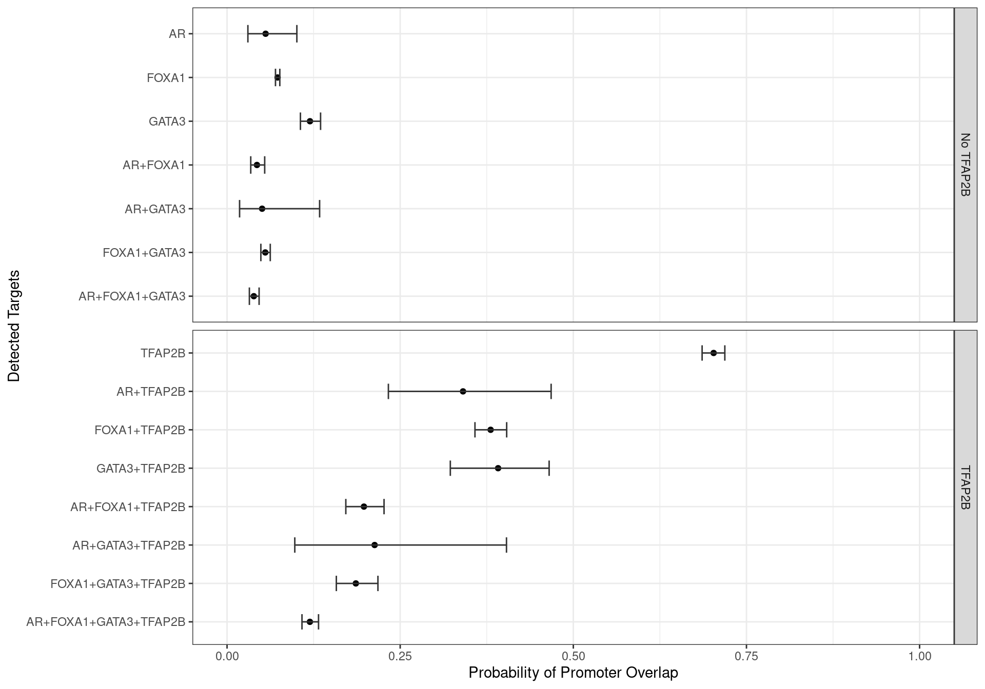
Family-wise 95% Confidence Intervals for the probability of overlapping an H3K27ac-derived promoter, based on the combinations of detected ChIP targets.
| Version | Author | Date |
|---|---|---|
| 1ba686b | Steve Pederson | 2022-05-19 |
Enhancers Only
grp_enh <- dht_consensus %>%
  as_tibble() %>%
  dplyr::select(range, all_of(targets), enhancer) %>%
  pivot_longer(cols = all_of(targets), names_to = "targets") %>%
  dplyr::filter(value) %>%
  group_by(range, enhancer) %>%
  summarise(targets = paste(targets, collapse = "+"), .groups = "drop")
glm_enh <- glm(enhancer ~ 0 + targets, family = "binomial", data = grp_enh)
glm_enh %>%
  glht() %>%
  confint() %>%
  .[["confint"]] %>%
  as_tibble(rownames = "targets") %>%
  mutate(
    n_targets = str_count(targets, "\\+") + 1
  ) %>%
  arrange(desc(n_targets), desc(targets)) %>%
  mutate(
    targets = fct_inorder(targets) %>%
      fct_relabel(str_remove_all, pattern = "targets"),
    p = inv.logit(Estimate),
    TFAP2B = ifelse(str_detect(targets, "TFAP2B"), "TFAP2B", "No TFAP2B"),
    across(all_of(c("upr", "lwr")), inv.logit)
  ) %>%
  ggplot(aes(p, targets)) +
  geom_point() +
  geom_errorbarh(aes(xmin = lwr, xmax = upr), height = 0.4, colour = "grey20") +
  facet_grid(TFAP2B ~ ., scales = "free_y") +
  scale_x_continuous(limits = c(0, 1)) +
  labs(x = "Probability of Enhancer Overlap", y = "Detected Targets")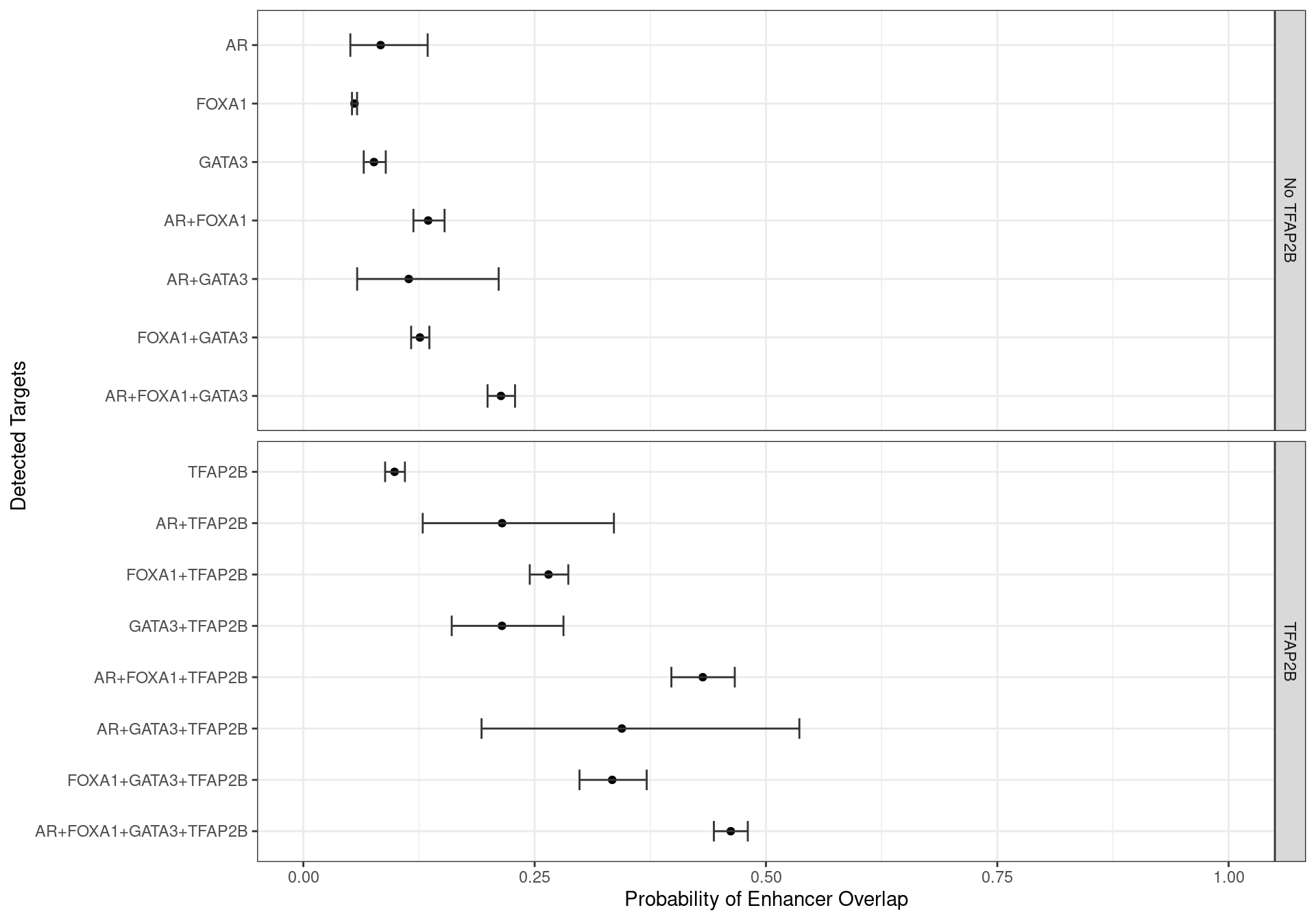
Family-wise 95% Confidence Intervals for the probability of overlapping an H3K27ac-derived enhancer, based on the combinations of detected ChIP targets.
| Version | Author | Date |
|---|---|---|
| 1ba686b | Steve Pederson | 2022-05-19 |
All Features
df <- dht_consensus %>%
  as_tibble() %>%
  mutate(
    ol = case_when(
      promoter ~ "Promoter",
      enhancer ~ "Enhancer",
      TRUE ~ "No H3K27ac"
    ) %>%
      fct_infreq()
  ) %>%
  pivot_longer(all_of(targets), names_to = "target") %>%
  dplyr::filter(value) %>%
  group_by(range, ol) %>%
  summarise(
    targets = paste(target, collapse = "+"),
    .groups = "drop"
  ) %>%
  mutate(n_targets = 1 + str_count(targets, "\\+")) %>%
  arrange(n_targets, targets) %>%
  mutate(targets = fct_inorder(targets))
glm_all <- multinom(ol~ 0 + targets, data = df)
ci_all <- Effect("targets", glm_all, confint = TRUE, confidence.level = 1 - 0.05/15)
list(
  tibble(targets = ci_all$variables$targets$levels) %>%
    bind_cols(ci_all$prob) %>%
    pivot_longer(starts_with("prob"), names_to = "ol") %>%
    mutate(ol = str_remove_all(ol, "prob."), type = "p"),
  tibble(targets = ci_all$variables$targets$levels) %>%
    bind_cols(ci_all$lower.prob) %>%
    pivot_longer(starts_with("L.prob"), names_to = "ol") %>%
    mutate(ol = str_remove_all(ol, "L.prob."), type = "lwr"),
  tibble(targets = ci_all$variables$targets$levels) %>%
    bind_cols(ci_all$upper.prob) %>%
    pivot_longer(starts_with("U.prob"), names_to = "ol") %>%
    mutate(ol = str_remove_all(ol, "U.prob."), type = "upr")
) %>%
  bind_rows() %>%
  pivot_wider(names_from = "type", values_from = value) %>%
  mutate(
    ol = str_replace_all(ol, "\\.", " ") %>% factor(levels = levels(df$ol)),
    TFAP2B = ifelse(str_detect(targets, "TFAP2B"), "TFAP2B", "No TFAP2B"),
    targets = factor(targets, levels = levels(df$targets)) %>%
      fct_relabel(str_remove_all, pattern = "\\+TFAP2B"),
    y = case_when(
      TFAP2B == "TFAP2B" ~ as.integer(targets) + 0.2,
      TFAP2B != "TFAP2B" ~ as.integer(targets) - 0.2
    )
  ) %>%
  # dplyr::filter(ol %in% c("Promoter", "Enhancer")) %>%
  ggplot(aes(p, y, colour = TFAP2B)) +
  geom_point() +
  geom_errorbarh(aes(xmin = lwr, xmax = upr), height = 0.25) +
  facet_grid(.~ol, scales = "free_y", space = "free") +
  scale_y_continuous(
    breaks = str_remove_all(levels(df$targets), "\\+TFAP2B") %>%
      unique() %>%
      seq_along(),
    labels = str_remove_all(levels(df$targets), "\\+TFAP2B") %>%
      unique()
  ) +
  scale_colour_manual(values = c("grey70", rgb(0.9, 0.1, 0.2))) +
  labs(
    x = expression(pi[i]),
    y = "Targets"
  )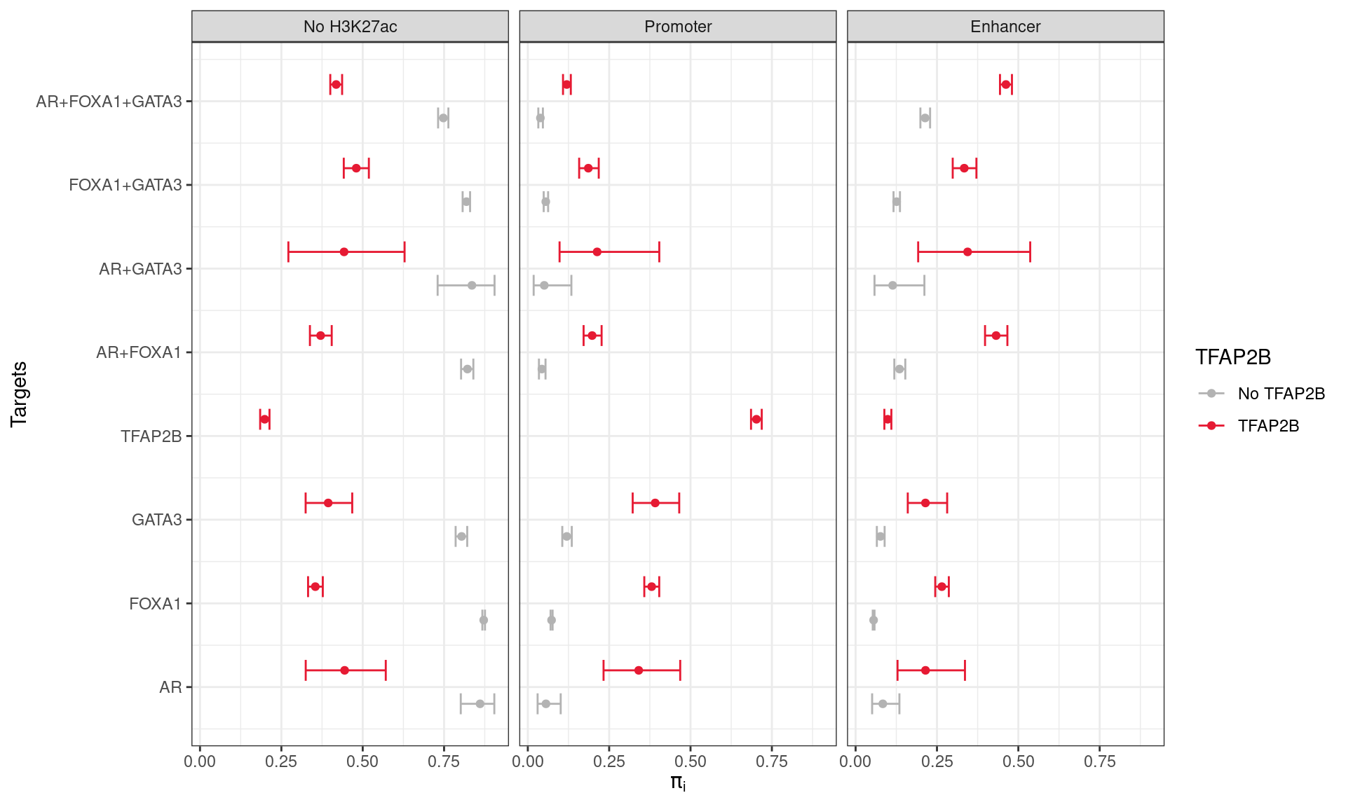
Probabilities of group membership for overlapping a promoter, enhancer, or having no H3K27ac overlap. Combinations of ChIP targets are shown based on coincident binding of TFAP2B. Intervals represent 1 - α Confidence Intervals, as described in the text. Co-binding of TFAP2β was strongly associated with an increased probability of a site being associated with H3K27ac peaks as defined previously.
| Version | Author | Date |
|---|---|---|
| 1ba686b | Steve Pederson | 2022-05-19 |
A simple multinomial model was then fit using the possible outcomes (or classes) for each site: 1) Promoter Overlap; 2) Enhancer Overlap, or 3) No H3K27ac overlap. \(1 - \alpha\) confidence intervals for the probability of class membership were then estimated using \(\alpha = 0.05/15\), given there were 15 combinations of transcription factors detected.
Distance to Nearest TSS
The distance to the nearest TSS was also checked for each of the union peaks, with the vast majority of TFAP2\(\beta\)-only peaks being with 1kb of a TSS, indicating a fundamental role for TFAP2\(\beta\) in transcriptional regulation. These were much further away when bound in combination with other ChIP targets, to the point that most sites where all four were found bound were >3kb from any TSS, suggesting that an alternative role for TFAP2\(\beta\) is enhancer-based gene regulation, when acting in concert with the remaining targets.
dht_consensus %>%
  as_tibble() %>%
  dplyr::select(range, all_of(targets), dist_to_tss, H3K27ac) %>%
  pivot_longer(cols = all_of(targets), names_to = "targets") %>%
  dplyr::filter(value) %>%
  group_by(range, dist_to_tss, H3K27ac) %>%
  arrange(range, targets) %>%
  summarise(targets = paste(targets, collapse = "+"), .groups = "drop") %>%
  mutate(
    n_targets = str_count(targets, "\\+") + 1,
    TFAP2B = ifelse(str_detect(targets, "TFAP2B"), "TFAP2B", "No TFAP2B")
  ) %>%
  arrange(desc(n_targets), desc(targets)) %>%
  mutate(targets = fct_inorder(targets)) %>%
  ggplot(aes(dist_to_tss + 1, targets, fill = H3K27ac)) +
  geom_boxplot() +
  facet_grid(TFAP2B ~ ., scales = "free_y") +
  # coord_cartesian(xlim = c(0, 5e4)) +
  scale_x_log10(labels = comma, breaks = 10^seq(0, 5)) +
  scale_fill_manual(values = c("grey70", rgb(0.9, 0.1, 0.2))) +
  labs(x = "Distance to Nearest TSS (bp+1)", y = "ChIP Targets")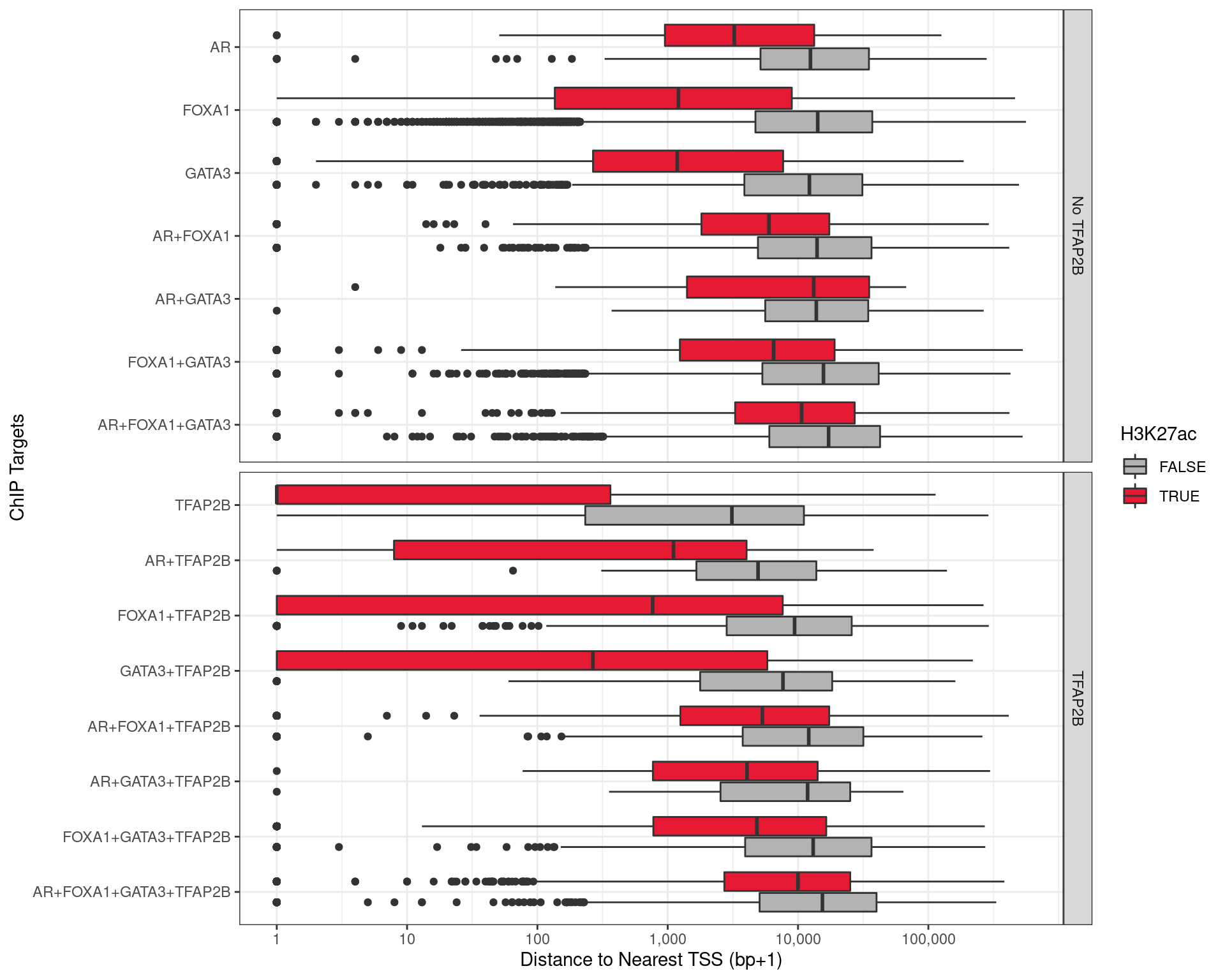
Distance to the nearest TSS for all peaks detected with one or more of the required ChIP targets.
dht_consensus %>%
  as_tibble() %>%
  # sample_n(10000) %>%
  dplyr::select(range, all_of(targets), dist_to_tss, H3K27ac) %>%
  pivot_longer(cols = all_of(targets), names_to = "targets") %>%
  dplyr::filter(value) %>%
  group_by(range, dist_to_tss, H3K27ac) %>%
  arrange(range, targets) %>%
  summarise(targets = paste(targets, collapse = "+"), .groups = "drop") %>%
  mutate(
    n_targets = str_count(targets, "\\+") + 1,
    TFAP2B = ifelse(str_detect(targets, "TFAP2B"), "TFAP2B", "No TFAP2B")
  ) %>%
  arrange(desc(n_targets), desc(targets)) %>%
  mutate(
    targets = str_remove_all(targets, "\\+TFAP2B"),
    targets = fct_inorder(targets)
  ) %>%
  ggplot(aes(dist_to_tss + 1, stat(density), colour = TFAP2B, linetype = H3K27ac)) +
  geom_density() +
  facet_wrap(.~targets) +
  scale_colour_manual(values = c("grey70", rgb(0.9, 0.1, 0.2))) +
  scale_linetype_manual(values = c(2, 1)) +
  scale_x_log10(labels = comma, breaks = 10^c(0:5))
Comparison With H3K27ac HiChIP Data
fl <- here::here("data", "hichip") %>%
  list.files(full.names = TRUE, pattern = "gi.+rds")
hic <- GInteractions()
for (f in fl) {
  hic <- c(hic, read_rds(f))
}
hic <- sort(hic)
H3K27ac-HiChIP obtained from SRA and analysed previously, was additionally included to improve mapping of peaks to genes. Whilst the previous H3K27ac-derived features were obtained from the same passages/experiments as GATA3 and AR, HiChIP data was obtained from a public dataset, not produced with the DRMCRL, and were defined using only the Vehicle controls from an Abemaciclib Vs. Vehicle experiment. Long range interactions were included for bin sizes of 5, 10, 20 and _40_kb. Before proceeding, the comparability of the H3K27ac-HiChIP and H3K27ac-derived features was checked. 93% of HiChIP long-range interactions overlapped a promoter or enhancer derived from H3K27ac ChIP-seq. Conversely, 86% or ChIP-Seq features mapped to a long-range interaction.
Comparison To Key Genes
data("grch37.cytobands")
tm <- read_rds(
  here::here("data", "annotations", "trans_models.rds")
)
bwfl <- list(
  AR = here::here("data", "bigwig", "AR") %>%
    list.files(pattern = "merged.+bw", full.names = TRUE) %>%
    BigWigFileList() %>%
    setNames(
      path(.) %>%
        basename() %>%
        str_remove_all("_merged_treat.+")
    ),
  FOXA1 = here::here("data", "bigwig", "FOXA1") %>%
    list.files(pattern = "merged.+bw", full.names = TRUE) %>%
    BigWigFileList() %>%
    setNames(
      path(.) %>%
        basename() %>%
        str_remove_all("_merged_treat.+")
    ),
  GATA3 = here::here("data", "bigwig", "GATA3") %>%
    list.files(pattern = "merged.+bw", full.names = TRUE) %>%
    BigWigFileList() %>%
    setNames(
      path(.) %>%
        basename() %>%
        str_remove_all("_merged_treat.+")
    ),
  TFAP2B = here::here("data", "bigwig", "TFAP2B") %>%
    list.files(pattern = "merged.+bw", full.names = TRUE) %>%
    BigWigFileList() %>%
    setNames(
      path(.) %>%
        basename() %>%
        str_remove_all("_merged_treat.+")
    ),
  H3K27ac = here::here("data", "bigwig", "H3K27ac") %>%
    list.files(pattern = "merged.+bw", full.names = TRUE) %>%
    BigWigFileList() %>%
    setNames(
      path(.) %>%
        basename() %>%
        str_extract("DHT|Veh")
    )
)
y_lim <- here::here("data", "bigwig", targets) %>%
  sapply(
    list.files, pattern = "merged.*summary", full.names= TRUE, simplify = FALSE
  ) %>%
  lapply(
    function(x) lapply(x, read_tsv)
  ) %>%
  lapply(bind_rows) %>%
  lapply(function(x) c(0, max(x$score))) %>%
  setNames(basename(names(.)))
y_lim$H3K27ac <- bwfl$H3K27ac %>%
  lapply(import.bw) %>%
  lapply(function(x) max(x$score)) %>%
  unlist() %>%
  max() %>%
  c(0) %>%
  range()
Mapping To Detected Genes
rnaseq <- here::here("data", "rnaseq", "dge.rds") %>%
  read_rds()
counts <- here::here("data", "rnaseq", "counts.out.gz") %>%
  read_tsv(skip = 1) %>%
  dplyr::select(Geneid, ends_with("bam"))
detected <- counts %>%
  pivot_longer(
    cols = ends_with("bam"), names_to = "sample", values_to = "counts"
  ) %>%
  mutate(detected = counts > 0) %>%
  group_by(Geneid) %>%
  summarise(detected = mean(detected) > 0.25, .groups = "drop") %>%
  dplyr::filter(detected) %>%
  pull("Geneid")
top_table <- here::here("data", "rnaseq", "MDA-MB-453_RNASeq.tsv") %>%
  read_tsv() # Not a DHT-treatment analysis though...
dht_consensus <- mapByFeature(
dht_consensus,
genes = subset(all_gr$gene, gene_id %in% detected),
prom = subset(features, feature == "promoter"),
## Given we have accuracte H3K27ac HiChIP, better mappings can be gained that way.
## Exclude any enhancers which overlap the HiChIP
enh = subset(features, feature == "enhancer") %>% filter_by_non_overlaps(hic),
gi = hic
) %>%
mutate(mapped = vapply(gene_id, function(x) length(x) > 0, logical(1)))
all_targets <- dht_consensus %>%
as_tibble() %>%
dplyr::filter(if_all(all_of(targets))) %>%
unnest(everything()) %>%
distinct(gene_id) %>%
pull("gene_id")In order to more accurately assign genes to actively transcribed genes, the RNA-Seq dataset generated in 2013 studying DHT Vs. Vehicle in MDA-MB-453 cells was used to define the set of genes able to be considered as detected. As this was a polyA dataset, some ncRNA which are not adenylated may be expressed, but will remain as undetected despite this technological limitation. All 21,328 genes with >1 read in at least 1/4 of the samples was considered to be detected, and peaks were only mapped to detected genes.
Mapping was performed using mapByFeature() from the
package extraChIP using:
- Promoters defined externally using H3K27ac
- Only the externally defined enhancers which contained no H3K27ac-HiChIP overlap
- H3K27ac HiChIP interactions for long range mapping
No separate enhancers were using in the mapping steps as the
H3K27ac-HiChIP interaction were considered to provide clear associations
between peaks and target genes. By contrast, the default mapping of
mapByFeature() would map all genes within 100kb to any peak
considered as an enhancer
90% of detected genes had one or more peaks mapped to them.
Looking specifically at the peaks for which all four targets directly overlapped, 10,250 of the 21,328 detected genes were mapped to at least one directly overlapping binding region.
MYC
As the gene MYC has been identified as a key target, the binding patterns within the gene were explored. The two binding sites with all four ChIP targets detected, within 100kb of MYC, and which were connected using HiChIP interactions were visualised and exported.
gr <- dht_consensus %>%
  filter(!!!syms(targets), mapped, enhancer) %>%
  filter(
    vapply(gene_name, function(x) "MYC" %in% x, logical(1))
  ) %>%
  mutate(d = distance(., subset(all_gr$gene, gene_name == "MYC"))) %>%
  arrange(d) %>%
  filter(d < 1e5)
fs <- 14
myc_plot <- plotHFGC(
  gr = gr,
  hic = hic %>%
    subsetByOverlaps(gr) %>%
    subsetByOverlaps(
      subset(all_gr$gene, gene_name == "MYC")
    ) %>%
    subset(as.integer(bin_size) <= 5e3),
  hicsize = 3,
  max = 5e7,
  genes = tm %>%
    mutate(detected = ifelse(gene %in% detected, "Detected", "Not-Detected")) %>%
    split(.$detected),
  genecol = c(
    Detected = "forestgreen", "Not-Detected" = rgb(0.2, 0.2, 0.7, 0.5)
  ),
  coverage = bwfl,
  linecol = c(targets, "H3K27ac") %>%
    sapply(function(x) {
      c(DHT = rgb(0.6, 0, 0), Veh = "grey60")
    },
    simplify = FALSE
    ),
  #ylim = lapply(y_lim, divide_by, e2 = 2),
  cytobands = grch37.cytobands,
  # collapseTranscripts = list(Detected = FALSE, `Not-Detected` = "meta"),
  zoom = 1.1,
  highlight = rgb(0, 0, 1, 0.5),
  title.width = 1,
  col.title = "black", background.title = "white",
  showAxis = FALSE,
  rotation.title = 90, fontsize = fs,
  fontface.title = 1,
  legend = FALSE,
  fontcolor.legend = "black"
)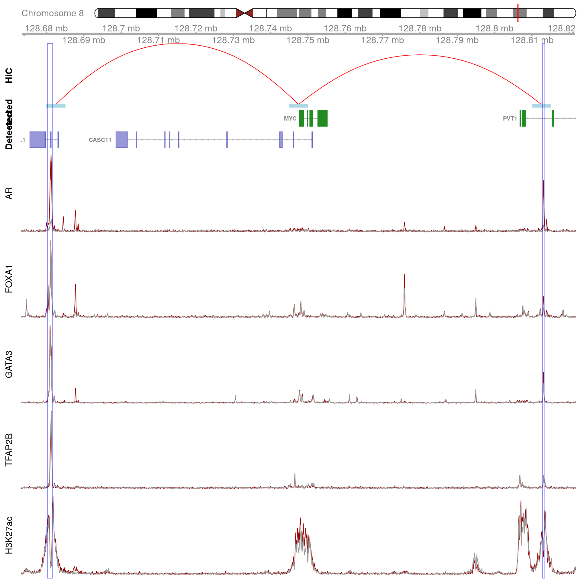
Two joint binding sites either side of MYC connected by HiChIP interactions to the promoter. HiChIP connections were detected at all bin sizes, however, only fine-resolutions 5kb interaction bins are shown.
myc_plot$chr8@dp@pars$fontcolor <- "black"
myc_plot$Axis@dp@pars$fontcolor <- "black"
myc_plot$Axis@dp@pars$col <- "grey30"
myc_plot$HiC@dp@pars$fontface.title <- 1
myc_plot$HiC@dp@pars$rotation.title <- 0
myc_plot$Detected@dp@pars$fontface.title <- 1
myc_plot$Detected@dp@pars$rotation.title <- 0
myc_plot$Detected@dp@pars$fontsize.group <- fs
myc_plot$Detected@dp@pars$cex.group <- 0.8
myc_plot$Detected@dp@pars$fontface.group <- 1
myc_plot$Detected@dp@pars$fontcolor.group <- "black"
myc_plot$`Not-Detected`@dp@pars$fontcolor.group <- "black"
myc_plot$`Not-Detected`@dp@pars$fontface.title <- 1
myc_plot$`Not-Detected`@dp@pars$rotation.title <- 0
myc_plot$`Not-Detected`@dp@pars$fontsize.group <- fs
myc_plot$`Not-Detected`@dp@pars$cex.group <- 0.8
myc_plot$`Not-Detected`@dp@pars$just.group <- "right"
myc_plot$`Not-Detected`@dp@pars$fontface.group <- 1
myc_plot$AR@dp@pars$rotation.title <- 0
myc_plot$FOXA1@dp@pars$rotation.title <- 0
myc_plot$GATA3@dp@pars$rotation.title <- 0
myc_plot$TFAP2B@dp@pars$rotation.title <- 0
myc_plot$H3K27ac@dp@pars$rotation.title <- 0
myc_plot$H3K27ac@dp@pars$legend <- TRUE
myc_plot$H3K27ac@dp@pars$size <- 5
ax <- myc_plot[1:2]
hl <- HighlightTrack(
  myc_plot[3:10],
  range = resize(gr, width = 2*width(gr), fix = 'center')
)
hl@dp@pars$fill <- rgb(1, 1, 1, 0)
hl@dp@pars$col <- "blue"
hl@dp@pars$lwd <- 0.5
pdf(here::here("output", "MYC.pdf"), width = 10, height = 10)
Gviz::plotTracks(
  c(ax, hl),
  myc_plot[1:10],
  from = min(start(gr)) - 0.1*width(range(gr)),
  to = max(end(gr)) + 0.1*width(range(gr)),
  title.width = 1,
  margin = 40,
  fontface.main = 1
  )
dev.off()
Apocrine Signature Enrichment
Subtype Gene Signatures
hgnc <- read_csv(
  here::here("data", "external", "hgnc-symbol-check.csv"), skip = 1
) %>%
  dplyr::select(Gene = Input, gene_name = `Approved symbol`)
apo_ranks <- here::here("data", "external", "ApoGenes.txt") %>%
  read_tsv() %>%
  left_join(hgnc) %>%
  left_join(
    as_tibble(all_gr$gene) %>%
      dplyr::select(gene_id, gene_name),
    by = "gene_name"
  ) %>%
  dplyr::select(starts_with("gene_"), ends_with("rank")) %>%
  dplyr::filter(!is.na(gene_id))
apo_full <- read_excel(
  here::here("data", "external", "Apocrine gene lists.xls"),
  col_names = c(
    "Gene",
    paste0("ESR1", c("_logFC", "_p")),
    paste0("CLCA2", c("_logFC", "_p")),
    paste0("DCN", c("_logFC", "_p")),
    paste0("GZMA", c("_logFC", "_p")),
    paste0("MX1", c("_logFC", "_p")),
    paste0("TPX2", c("_logFC", "_p")),
    paste0("FABP4", c("_logFC", "_p")),
    paste0("ADM", c("_logFC", "_p")),
    paste0("CD83", c("_logFC", "_p"))
    ),
  col_types = c("text", rep("numeric", 18)),
  skip = 1
) %>%
  left_join(hgnc) %>%
  left_join(
    as_tibble(all_gr$gene) %>%
      dplyr::select(gene_id, gene_name),
    by = "gene_name"
  ) %>%
  dplyr::select(starts_with("gene", FALSE), matches("_(logFC|p)"))
apo_genesets <- colnames(apo_full) %>%
  str_subset("_p$") %>%
  sapply(
    function(x) {
      dplyr::filter(apo_full, !!sym(x) < 0.05, !is.na(gene_name))$gene_name
    },
    simplify = FALSE
  ) %>%
  setNames(
    str_remove(names(.), pattern = "_p")
  )
genes_by_subtype <- apo_genesets %>%
  lapply(list) %>%
  as_tibble() %>%
  pivot_longer(everything(), names_to = "subtype", values_to = "gene_name") %>%
  unnest(everything()) %>%
  split(.$gene_name) %>%
  lapply(pull, "subtype")
The models for different subtypes, as previously published were loaded, with a signature from each subtype being derived from genes with an adjusted p-value < 0.05, as initially published. This gave 9 different gene-sets with key marker genes denoting the subtypes: ESR1, CLCA2, DCN, GZMA, MX1, TPX2, FABP4, ADM and CD83
apo_genesets %>%
  fromList() %>%
  upset(
    sets = rev(names(.)),
    # keep.order = TRUE,
    order.by = "freq",
    set_size.show = TRUE,
    set_size.scale_max = nrow(.) * 0.4
  )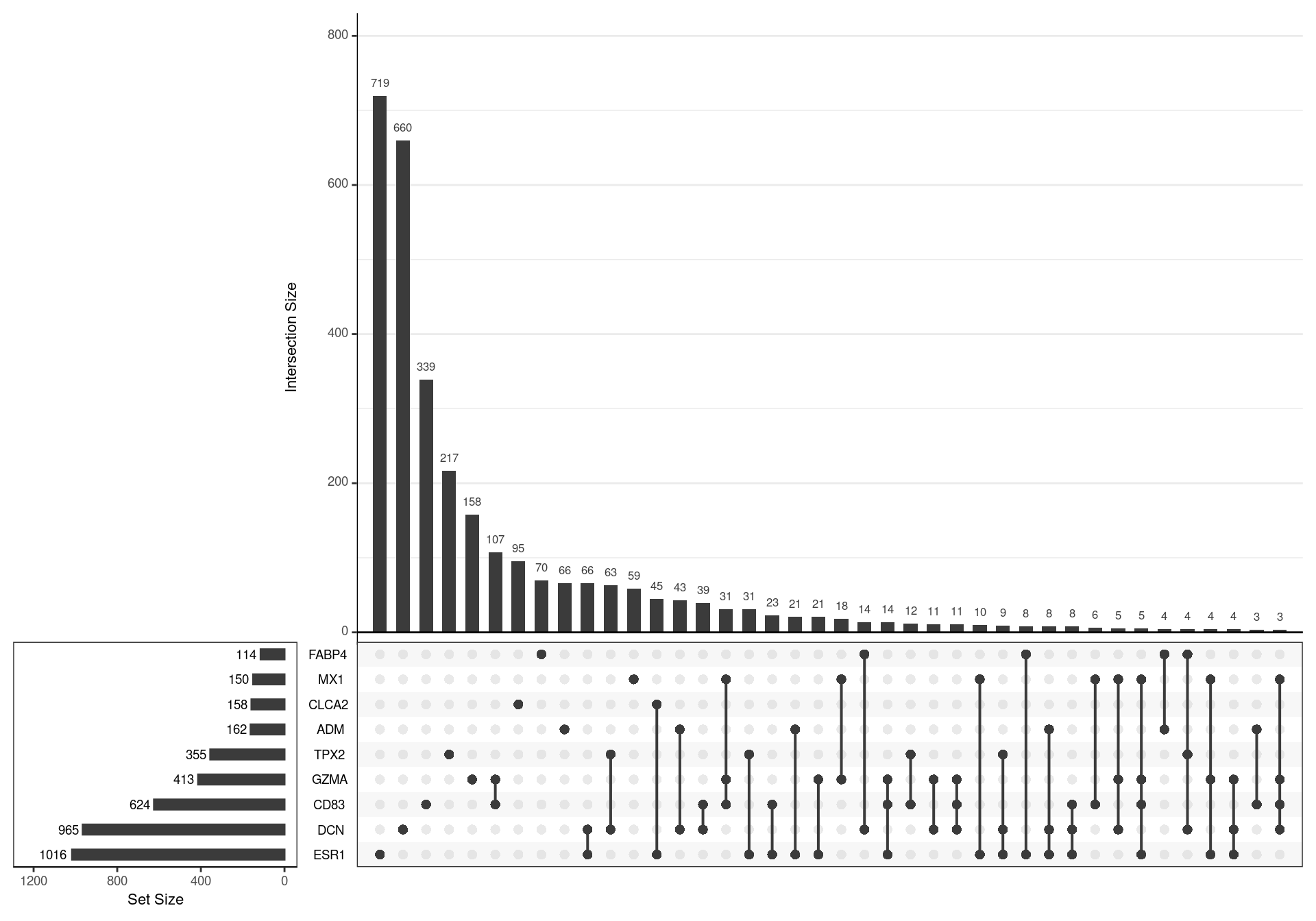
UpSet plot showing the association between genes contained in each signature. A relatively high degree of similarity was noted between some signature pairs, such as GZMA/CD83 and MX1/GZMA
apo_genesets %>%
  fromList() %>%
  cor() %>%
  corrplot(
    diag = FALSE,
    addCoef.col = "grey50",
    addCoefasPercent = TRUE
  )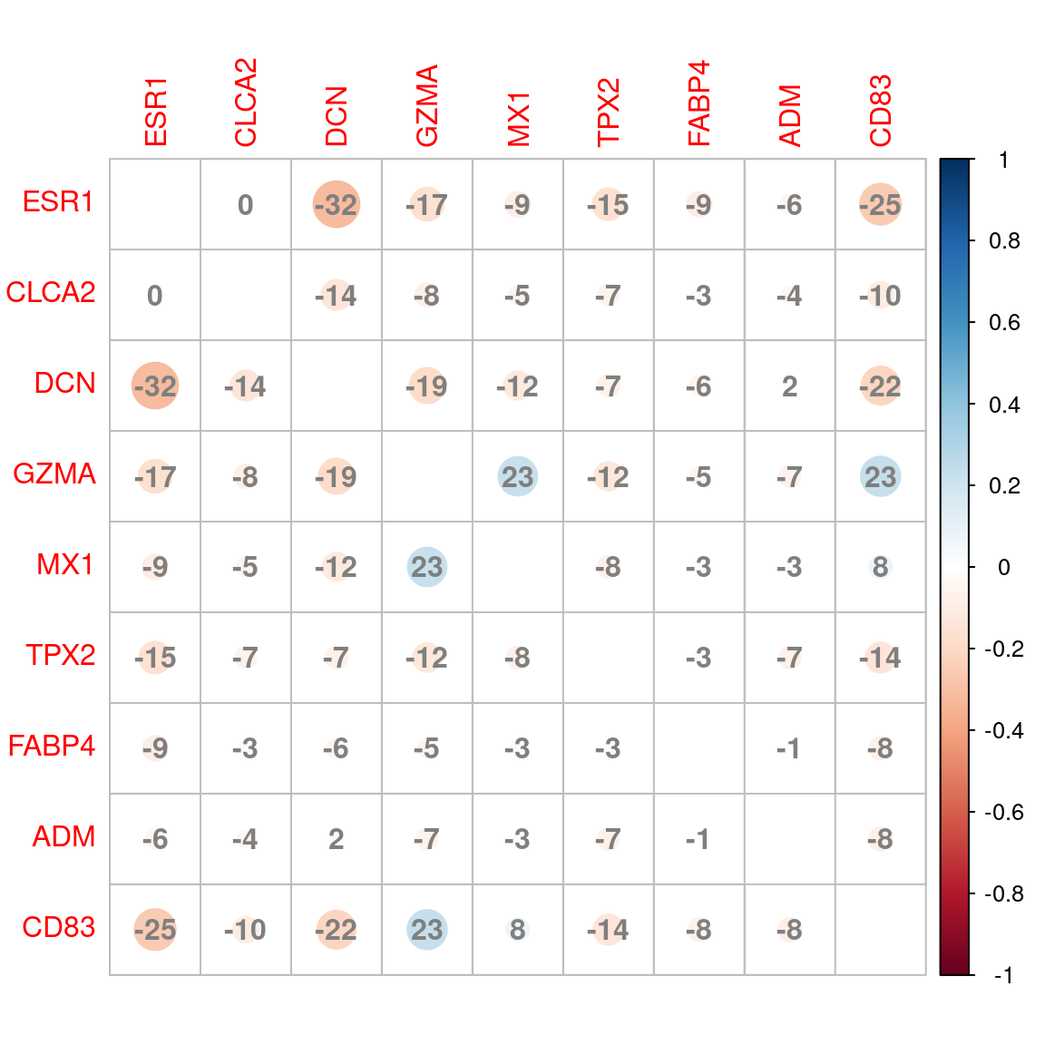
Correlation plot between signatures based on shared genes between groups
Enrichment Testing: All Sites
The set of genes mapped to sites contain all four ChIP targets were
then tested for enrichment of any of the defined signatures. Enrichment
testing as implemented in goseq was used, incorporating the
number of consensus peaks mapped to a gene as the offset term for biased
sampling.
mapped <- all_gr$gene %>%
  filter(gene_id %in% detected) %>%
  mutate(gene_width = width) %>%
  as_tibble() %>%
  dplyr::select(starts_with("gene")) %>%
  mutate(
    mapped_to_all = gene_name %in% unlist(filter(dht_consensus, !!!syms(targets))$gene_name),
    n_peaks = table(unlist(dht_consensus$gene_name))[gene_name] %>%
      as.integer(),
    n_peaks = ifelse(is.na(n_peaks), 0, n_peaks)
  ) %>%
  distinct(gene_name, .keep_all = TRUE)
goseq_all4 <- structure(
  mapped$mapped_to_all, names = mapped$gene_name
) %>%
  nullp(bias.data = mapped$n_peaks) %>%
  goseq(gene2cat = genes_by_subtype) %>%
  as_tibble() %>%
  dplyr::select(
    subtype = category,
    p = over_represented_pvalue,
    n_mapped = numDEInCat,
    signature_size = numInCat
  ) %>%
  mutate(fdr = p.adjust(p, "fdr"))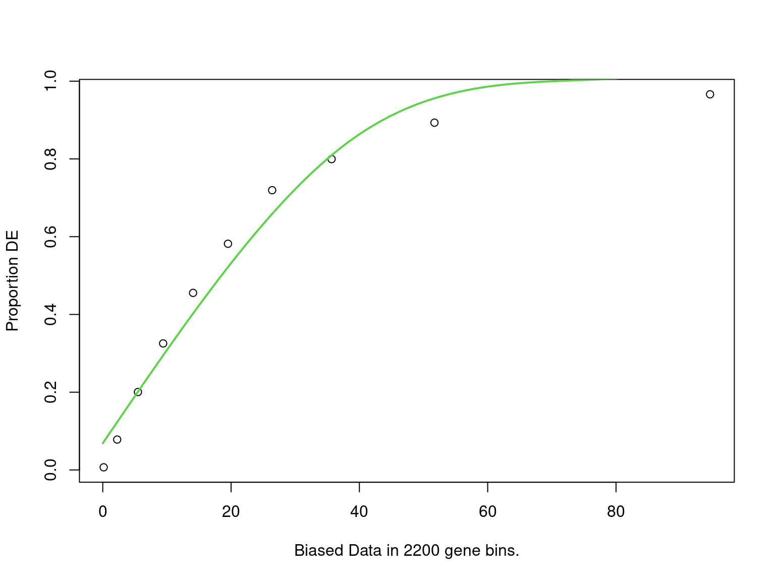
PWF for biased sampling using the number of peaks mapped to a gene as the bias offset
goseq_all4 %>%
  mutate(`%` = percent(n_mapped / signature_size, accuracy = 0.1)) %>%
  dplyr::select(
    Subtype = subtype, `Signature Size` = signature_size, `# Mapped` = n_mapped,
    `% Mapped` = `%`, p, FDR = fdr
  ) %>%
  pander(
    justify = "lrrrrr",
    caption = paste(
      "Results for Subtype enrichment testing using all genes mapped to any ",
      "consensus peak, where all four ChIP targets were considered to be present."
    ),
    emphasize.strong.rows = which(.$FDR < 0.05)
)| Subtype | Signature Size | # Mapped | % Mapped | p | FDR |
|---|---|---|---|---|---|
| CLCA2 | 136 | 104 | 76.5% | 0.001183 | 0.01065 |
| ESR1 | 868 | 538 | 62.0% | 0.07247 | 0.3261 |
| ADM | 123 | 75 | 61.0% | 0.1586 | 0.4759 |
| TPX2 | 333 | 206 | 61.9% | 0.3267 | 0.735 |
| DCN | 766 | 443 | 57.8% | 0.7412 | 0.9502 |
| FABP4 | 50 | 22 | 44.0% | 0.9141 | 0.9502 |
| GZMA | 195 | 97 | 49.7% | 0.9372 | 0.9502 |
| CD83 | 400 | 210 | 52.5% | 0.9445 | 0.9502 |
| MX1 | 106 | 47 | 44.3% | 0.9502 | 0.9502 |
Enrichment Testing: H3K27Ac-Associated
The same process was then performed restricting the mappings to those sites associated with H3K27ac binding.
mapped_h3k <- all_gr$gene %>%
  filter(gene_id %in% detected) %>%
  mutate(gene_width = width) %>%
  as_tibble() %>%
  dplyr::select(starts_with("gene")) %>%
  mutate(
    mapped_to_all = gene_name %in% unlist(filter(dht_consensus, !!!syms(targets), H3K27ac)$gene_name),
    n_peaks = table(unlist(dht_consensus$gene_name))[gene_name] %>%
      as.integer(),
    n_peaks = ifelse(is.na(n_peaks), 0, n_peaks)
  ) %>%
  distinct(gene_name, .keep_all = TRUE)
goseq_h3k <- structure(
  mapped_h3k$mapped_to_all, names = mapped_h3k$gene_name
) %>%
  nullp(bias.data = mapped_h3k$n_peaks) %>%
  goseq(gene2cat = genes_by_subtype) %>%
  as_tibble() %>%
  dplyr::select(
    subtype = category,
    p = over_represented_pvalue,
    n_mapped = numDEInCat,
    signature_size = numInCat
  ) %>%
  mutate(fdr = p.adjust(p, "fdr"))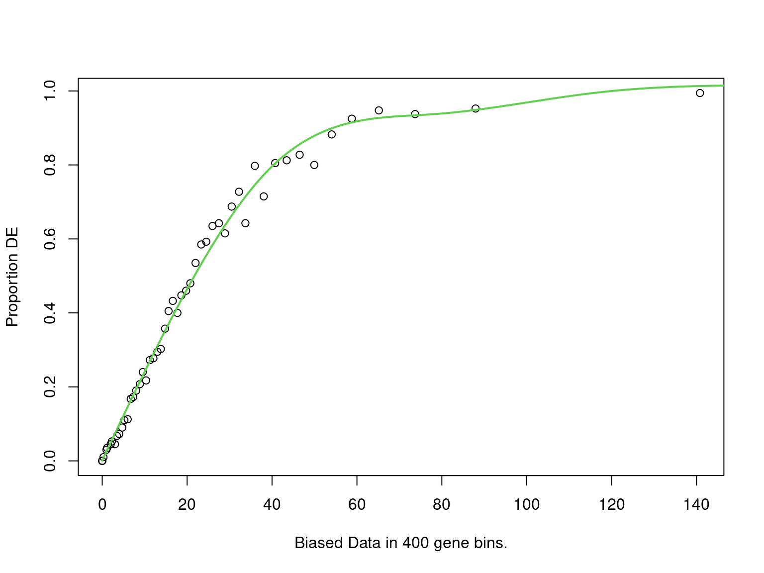
PWF for biased sampling using the number of peaks mapped to a gene as the bias offset
goseq_h3k %>%
  mutate(`%` = percent(n_mapped / signature_size, accuracy = 0.1)) %>%
  dplyr::select(
    Subtype = subtype, `Signature Size` = signature_size, `# Mapped` = n_mapped,
    `% Mapped` = `%`, p, FDR = fdr
  ) %>%
  pander(
    justify = "lrrrrr",
    caption = paste(
      "Results for Subtype enrichment testing using only genes mapped to a",
      "consensus peak *associated with H3K27ac activity*, and where all four",
      "ChIP targets were considered to be present."
    ),
    emphasize.strong.rows = which(.$FDR < 0.05)
)| Subtype | Signature Size | # Mapped | % Mapped | p | FDR |
|---|---|---|---|---|---|
| CLCA2 | 136 | 99 | 72.8% | 3.783e-05 | 0.0003405 |
| ESR1 | 868 | 479 | 55.2% | 0.006078 | 0.02735 |
| ADM | 123 | 64 | 52.0% | 0.183 | 0.5491 |
| TPX2 | 333 | 177 | 53.2% | 0.4041 | 0.9092 |
| FABP4 | 50 | 19 | 38.0% | 0.8337 | 0.9899 |
| MX1 | 106 | 39 | 36.8% | 0.9165 | 0.9899 |
| GZMA | 195 | 81 | 41.5% | 0.9184 | 0.9899 |
| DCN | 766 | 366 | 47.8% | 0.9617 | 0.9899 |
| CD83 | 400 | 169 | 42.2% | 0.9899 | 0.9899 |
sessionInfo()R version 4.2.0 (2022-04-22)
Platform: x86_64-pc-linux-gnu (64-bit)
Running under: Ubuntu 20.04.4 LTS
Matrix products: default
BLAS: /usr/lib/x86_64-linux-gnu/blas/libblas.so.3.9.0
LAPACK: /usr/lib/x86_64-linux-gnu/lapack/liblapack.so.3.9.0
locale:
[1] LC_CTYPE=en_AU.UTF-8 LC_NUMERIC=C
[3] LC_TIME=en_AU.UTF-8 LC_COLLATE=en_AU.UTF-8
[5] LC_MONETARY=en_AU.UTF-8 LC_MESSAGES=en_AU.UTF-8
[7] LC_PAPER=en_AU.UTF-8 LC_NAME=C
[9] LC_ADDRESS=C LC_TELEPHONE=C
[11] LC_MEASUREMENT=en_AU.UTF-8 LC_IDENTIFICATION=C
attached base packages:
[1] grid stats4 stats graphics grDevices utils datasets
[8] methods base
other attached packages:
[1] goseq_1.48.0 geneLenDataBase_1.32.0
[3] BiasedUrn_1.07 corrplot_0.92
[5] readxl_1.4.0 Gviz_1.40.1
[7] effects_4.2-1 carData_3.0-5
[9] nnet_7.3-17 glue_1.6.2
[11] multcomp_1.4-19 TH.data_1.1-1
[13] MASS_7.3-56 survival_3.2-13
[15] mvtnorm_1.1-3 GenomicInteractions_1.30.0
[17] InteractionSet_1.24.0 rtracklayer_1.56.0
[19] UpSetR_1.4.0 htmltools_0.5.2
[21] reactable_0.2.3 scales_1.2.0
[23] pander_0.6.5 plyranges_1.16.0
[25] extraChIPs_1.0.0 SummarizedExperiment_1.26.1
[27] Biobase_2.56.0 MatrixGenerics_1.8.0
[29] matrixStats_0.62.0 GenomicRanges_1.48.0
[31] GenomeInfoDb_1.32.1 IRanges_2.30.0
[33] S4Vectors_0.34.0 BiocGenerics_0.42.0
[35] BiocParallel_1.30.0 magrittr_2.0.3
[37] forcats_0.5.1 stringr_1.4.0
[39] dplyr_1.0.9 purrr_0.3.4
[41] readr_2.1.2 tidyr_1.2.0
[43] tibble_3.1.7 ggplot2_3.3.6
[45] tidyverse_1.3.1 workflowr_1.7.0
loaded via a namespace (and not attached):
[1] rappdirs_0.3.3 csaw_1.30.0 bit64_4.0.5
[4] knitr_1.39 DelayedArray_0.22.0 data.table_1.14.2
[7] rpart_4.1.16 KEGGREST_1.36.0 RCurl_1.98-1.6
[10] AnnotationFilter_1.20.0 doParallel_1.0.17 generics_0.1.2
[13] GenomicFeatures_1.48.0 callr_3.7.0 EnrichedHeatmap_1.26.0
[16] RSQLite_2.2.14 bit_4.0.4 tzdb_0.3.0
[19] xml2_1.3.3 lubridate_1.8.0 httpuv_1.6.5
[22] assertthat_0.2.1 xfun_0.31 hms_1.1.1
[25] jquerylib_0.1.4 evaluate_0.15 promises_1.2.0.1
[28] fansi_1.0.3 restfulr_0.0.13 progress_1.2.2
[31] dbplyr_2.1.1 igraph_1.3.1 DBI_1.1.2
[34] htmlwidgets_1.5.4 ellipsis_0.3.2 crosstalk_1.2.0
[37] backports_1.4.1 insight_0.17.1 survey_4.1-1
[40] biomaRt_2.52.0 vctrs_0.4.1 here_1.0.1
[43] ensembldb_2.20.1 cachem_1.0.6 withr_2.5.0
[46] ggforce_0.3.3 BSgenome_1.64.0 vroom_1.5.7
[49] checkmate_2.1.0 GenomicAlignments_1.32.0 prettyunits_1.1.1
[52] cluster_2.1.3 lazyeval_0.2.2 crayon_1.5.1
[55] labeling_0.4.2 edgeR_3.38.0 pkgconfig_2.0.3
[58] tweenr_1.0.2 nlme_3.1-157 ProtGenerics_1.28.0
[61] rlang_1.0.2 lifecycle_1.0.1 sandwich_3.0-1
[64] filelock_1.0.2 BiocFileCache_2.4.0 modelr_0.1.8
[67] dichromat_2.0-0.1 cellranger_1.1.0 rprojroot_2.0.3
[70] polyclip_1.10-0 reactR_0.4.4 Matrix_1.4-1
[73] boot_1.3-28 zoo_1.8-10 reprex_2.0.1
[76] base64enc_0.1-3 whisker_0.4 GlobalOptions_0.1.2
[79] processx_3.5.3 png_0.1-7 rjson_0.2.21
[82] bitops_1.0-7 getPass_0.2-2 Biostrings_2.64.0
[85] blob_1.2.3 shape_1.4.6 jpeg_0.1-9
[88] memoise_2.0.1 plyr_1.8.7 zlibbioc_1.42.0
[91] compiler_4.2.0 scatterpie_0.1.7 BiocIO_1.6.0
[94] RColorBrewer_1.1-3 clue_0.3-60 lme4_1.1-29
[97] Rsamtools_2.12.0 cli_3.3.0 XVector_0.36.0
[100] ps_1.7.0 htmlTable_2.4.0 Formula_1.2-4
[103] mgcv_1.8-40 ggside_0.2.0.9990 tidyselect_1.1.2
[106] stringi_1.7.6 highr_0.9 mitools_2.4
[109] yaml_2.3.5 locfit_1.5-9.5 latticeExtra_0.6-29
[112] ggrepel_0.9.1 sass_0.4.1 VariantAnnotation_1.42.0
[115] tools_4.2.0 parallel_4.2.0 circlize_0.4.15
[118] rstudioapi_0.13 foreach_1.5.2 foreign_0.8-82
[121] git2r_0.30.1 metapod_1.4.0 gridExtra_2.3
[124] farver_2.1.0 digest_0.6.29 Rcpp_1.0.8.3
[127] broom_0.8.0 later_1.3.0 httr_1.4.3
[130] AnnotationDbi_1.58.0 biovizBase_1.44.0 ComplexHeatmap_2.12.0
[133] colorspace_2.0-3 rvest_1.0.2 XML_3.99-0.9
[136] fs_1.5.2 splines_4.2.0 jsonlite_1.8.0
[139] nloptr_2.0.1 ggfun_0.0.6 R6_2.5.1
[142] Hmisc_4.7-0 pillar_1.7.0 fastmap_1.1.0
[145] minqa_1.2.4 codetools_0.2-18 utf8_1.2.2
[148] lattice_0.20-45 bslib_0.3.1 curl_4.3.2
[151] GO.db_3.15.0 limma_3.52.0 rmarkdown_2.14
[154] munsell_0.5.0 GetoptLong_1.0.5 GenomeInfoDbData_1.2.8
[157] iterators_1.0.14 haven_2.5.0 gtable_0.3.0