Deconvolution
Dongyue Xie
2019-12-10
Last updated: 2020-03-13
Checks: 7 0
Knit directory: misc/
This reproducible R Markdown analysis was created with workflowr (version 1.6.0). The Checks tab describes the reproducibility checks that were applied when the results were created. The Past versions tab lists the development history.
Great! Since the R Markdown file has been committed to the Git repository, you know the exact version of the code that produced these results.
Great job! The global environment was empty. Objects defined in the global environment can affect the analysis in your R Markdown file in unknown ways. For reproduciblity it’s best to always run the code in an empty environment.
The command set.seed(20191122) was run prior to running the code in the R Markdown file. Setting a seed ensures that any results that rely on randomness, e.g. subsampling or permutations, are reproducible.
Great job! Recording the operating system, R version, and package versions is critical for reproducibility.
Nice! There were no cached chunks for this analysis, so you can be confident that you successfully produced the results during this run.
Great job! Using relative paths to the files within your workflowr project makes it easier to run your code on other machines.
Great! You are using Git for version control. Tracking code development and connecting the code version to the results is critical for reproducibility. The version displayed above was the version of the Git repository at the time these results were generated.
Note that you need to be careful to ensure that all relevant files for the analysis have been committed to Git prior to generating the results (you can use wflow_publish or wflow_git_commit). workflowr only checks the R Markdown file, but you know if there are other scripts or data files that it depends on. Below is the status of the Git repository when the results were generated:
Ignored files:
    Ignored:    .Rhistory
    Ignored:    .Rproj.user/

Untracked files:
    Untracked:  analysis/gsea.Rmd
    Untracked:  analysis/ideas.Rmd
    Untracked:  analysis/methylation.Rmd
    Untracked:  analysis/susie.Rmd
    Untracked:  code/sccytokines.R
    Untracked:  code/scdeCalibration.R
    Untracked:  data/bart/
    Untracked:  data/cytokine/DE_controls_output_filter10.RData
    Untracked:  data/cytokine/DE_controls_output_filter10_addlimma.RData
    Untracked:  data/cytokine/README
    Untracked:  data/cytokine/test.RData
    Untracked:  data/cytokine_normalized.RData
    Untracked:  data/deconv/
    Untracked:  data/scde/

Unstaged changes:
    Deleted:    data/mout_high.RData
    Deleted:    data/scCDT.RData
    Deleted:    data/sva_sva_high.RData
Note that any generated files, e.g. HTML, png, CSS, etc., are not included in this status report because it is ok for generated content to have uncommitted changes.
These are the previous versions of the R Markdown and HTML files. If you’ve configured a remote Git repository (see ?wflow_git_remote), click on the hyperlinks in the table below to view them.
| File | Version | Author | Date | Message |
|---|---|---|---|---|
| Rmd | 73933a7 | DongyueXie | 2020-03-13 | wflow_publish(“analysis/deconvolution.Rmd”) |
| html | 53cef0f | Dongyue Xie | 2019-12-10 | Build site. |
| Rmd | af20c49 | Dongyue Xie | 2019-12-10 | wflow_publish(“analysis/deconvolution.Rmd”) |
Introduction
We have scRNA-seq data from Segerstolpe et al. (2016) including the 1097 cells from 6 healthy subjects, taken from here. In the following simulation study, 4 cell types - acinar, alpha, beta, and ductal cells are included.
EMTAB.eset = readRDS('data/deconv/EMTABesethealthy.rds')
EMTAB.eset
Loading required package: BiobaseLoading required package: BiocGenericsLoading required package: parallel
Attaching package: 'BiocGenerics'The following objects are masked from 'package:parallel':
clusterApply, clusterApplyLB, clusterCall, clusterEvalQ,
clusterExport, clusterMap, parApply, parCapply, parLapply,
parLapplyLB, parRapply, parSapply, parSapplyLBThe following objects are masked from 'package:stats':
IQR, mad, sd, var, xtabsThe following objects are masked from 'package:base':
anyDuplicated, append, as.data.frame, basename, cbind,
colMeans, colnames, colSums, dirname, do.call, duplicated,
eval, evalq, Filter, Find, get, grep, grepl, intersect,
is.unsorted, lapply, lengths, Map, mapply, match, mget, order,
paste, pmax, pmax.int, pmin, pmin.int, Position, rank, rbind,
Reduce, rowMeans, rownames, rowSums, sapply, setdiff, sort,
table, tapply, union, unique, unsplit, which, which.max,
which.minWelcome to Bioconductor
Vignettes contain introductory material; view with
'browseVignettes()'. To cite Bioconductor, see
'citation("Biobase")', and for packages 'citation("pkgname")'.ExpressionSet (storageMode: lockedEnvironment)
assayData: 25453 features, 1097 samples
element names: exprs
protocolData: none
phenoData
sampleNames: AZ_A10 AZ_A11 ... HP1509101_P9 (1097 total)
varLabels: sampleID SubjectName cellTypeID cellType
varMetadata: labelDescription
featureData: none
experimentData: use 'experimentData(object)'
Annotation: table(EMTAB.eset$cellType)
                acinar                  alpha                   beta
                   112                    443                    171
         co-expression                  delta                 ductal
                    26                     59                    135
           endothelial                epsilon                  gamma
                    13                      5                     75
                  mast           MHC class II                    PSC
                     4                      1                     23
          unclassified unclassified endocrine
                     1                     29
Now obtain the true gene relative expression in each cell type.
Preprocess the data: 1. remove genes appearing in less than 10 cells; 2. remove top \(1\%\) expressed genes
cell_types = c('acinar','alpha','beta','ductal')

#remove genes appeared in too few cells
#remove genes that are overly expressed
rm.idx = which(rowSums((exprs(EMTAB.eset)[,which(EMTAB.eset$cellType%in%cell_types)])!=0)<10)
rr = rowSums((exprs(EMTAB.eset)[,which(EMTAB.eset$cellType%in%cell_types)]))
#rm.idx = which(rr==0)
#rm.idx1 = which(rr<=quantile(rr[-rm.idx],0.01))
rm.idx2 = which(rr>=quantile(rr[-rm.idx],0.95))
rm.idx = unique(c(rm.idx,rm.idx2))

acinar = exprs(EMTAB.eset)[-rm.idx,which(EMTAB.eset$cellType=='acinar')]
alpha = exprs(EMTAB.eset)[-rm.idx,which(EMTAB.eset$cellType=='alpha')]
beta = exprs(EMTAB.eset)[-rm.idx,which(EMTAB.eset$cellType=='beta')]
ductal = exprs(EMTAB.eset)[-rm.idx,which(EMTAB.eset$cellType=='ductal')]
Check cell library size: cell library sizes are big
summary(colSums(acinar)) Min. 1st Qu. Median Mean 3rd Qu. Max.
5565 76099 140386 232418 328637 981553 summary(colSums(alpha)) Min. 1st Qu. Median Mean 3rd Qu. Max.
5842 65225 134546 184102 261253 1165737 summary(colSums(beta)) Min. 1st Qu. Median Mean 3rd Qu. Max.
4871 79238 164028 206068 316283 846231 summary(colSums(ductal)) Min. 1st Qu. Median Mean 3rd Qu. Max.
11119 67514 155453 242885 341715 1333342 # cell type specific gene relative expression
Theta = cbind(rowSums(acinar)/sum(acinar),
rowSums(alpha)/sum(alpha),
rowSums(beta)/sum(beta),
rowSums(ductal)/sum(ductal))
cor(Theta) [,1] [,2] [,3] [,4]
[1,] 1.0000000 0.5215232 0.4614900 0.6805119
[2,] 0.5215232 1.0000000 0.7833674 0.5356580
[3,] 0.4614900 0.7833674 1.0000000 0.4803255
[4,] 0.6805119 0.5356580 0.4803255 1.0000000kappa(t(Theta)%*%Theta)[1] 16.63482# cell size
S = c(sum(acinar)/ncol(acinar),
sum(alpha)/ncol(alpha),
sum(beta)/ncol(beta),
sum(ductal)/ncol(ductal))
S=S/100
set.seed(12345)
# bulk data library size: 50*number of genes.
bulk_ls = 50*nrow(Theta)
# total number of cells in bulk data
bulk_ncell = 400
# cell proportions
bulk_beta = c(1,2,3,4)
bulk_beta = bulk_beta/sum(bulk_beta)
# bulk data gene relative expression.
bulk_X = bulk_ncell*Theta%*%diag(S)%*%bulk_beta
bulk_theta = bulk_X/sum(bulk_X)
ref_ncell = 100
ref_X = Theta%*%diag(S)*ref_ncell
w = rep(1,length(bulk_theta))
ci_l = c()
ci_r = c()
beta_est = c()
for(rep in 1:100){
Z = matrix(rpois(prod(dim(ref_X)),ref_X),ncol=ncol(ref_X))
y = rpois(length(bulk_theta),bulk_ls*bulk_theta)
#W = diag(w)
#beta_hat = solve(t(Z)%*%W%*%Z - diag(colSums(W%*%Z)))%*%t(Z)%*%W%*%y
beta_hat = solve(t(Z)%*%Z - diag(colSums(Z)))%*%t(Z)%*%y
#beta_hat = solve(t(Z)%*%Z)%*%t(Z)%*%y
#beta_hat
#beta_hat/sum(beta_hat)
Q = 0
Sigma=0
for(i in 1:length(y)){
ag = Z[i,]%*%t(Z[i,])-diag(Z[i,])
Q = Q + ag
Delta = (ag%*%beta_hat-y[i]*Z[i,])
Sigma = Sigma + Delta%*%t(Delta)
}
Q = Q*2/length(y)
Sigma = Sigma*4/length(y)
K = ncol(Z)
J = matrix(nrow = ncol(Z),ncol=ncol(Z))
for(i in 1:K){
for(j in 1:K){
if(i==j){
J[i,j] = sum(beta_hat)-beta_hat[i]
}else{
J[i,j] = -beta_hat[i]
}
}
}
asyV = J%*%solve(Q)%*%Sigma%*%solve(Q)%*%J
beta_est = rbind(beta_est,c(beta_hat))
ci_l = cbind(ci_l,beta_hat/sum(beta_hat)-2*sqrt(diag(asyV)/length(y)))
ci_r = cbind(ci_r,beta_hat/sum(beta_hat)+2*sqrt(diag(asyV)/length(y)))
}
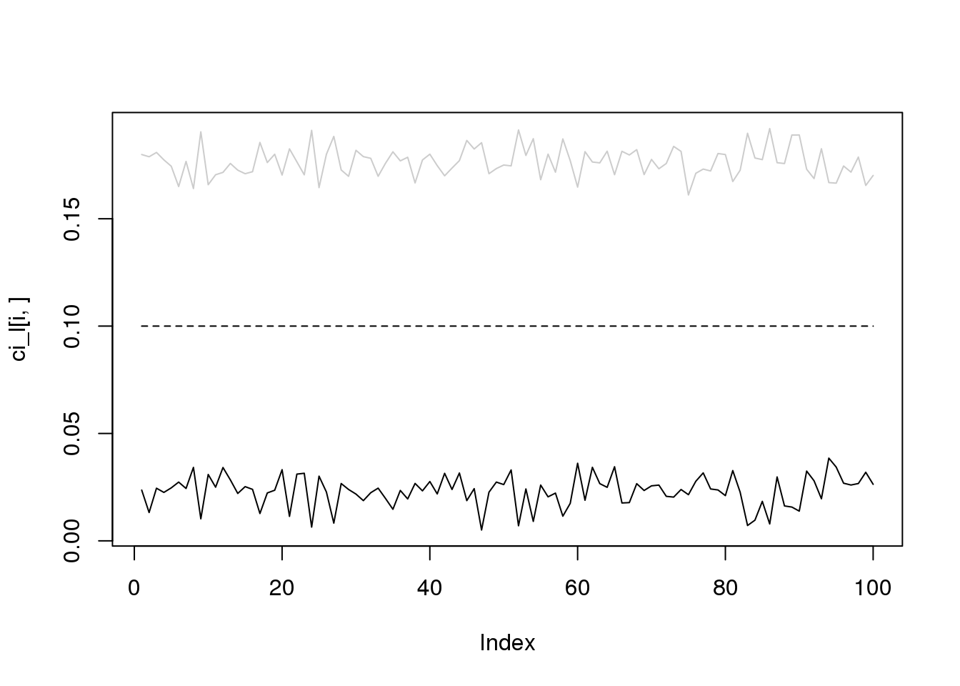
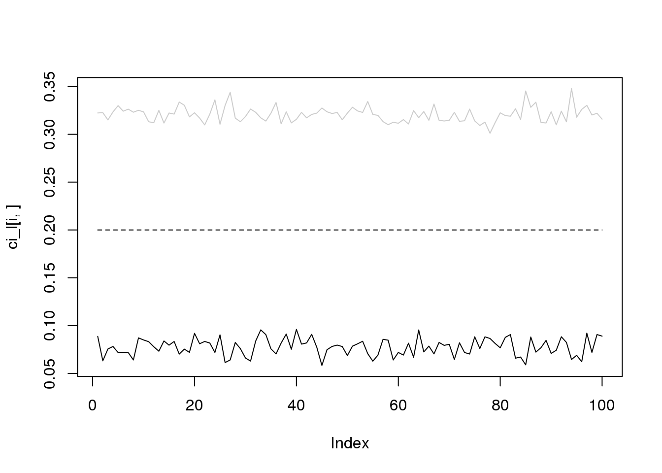
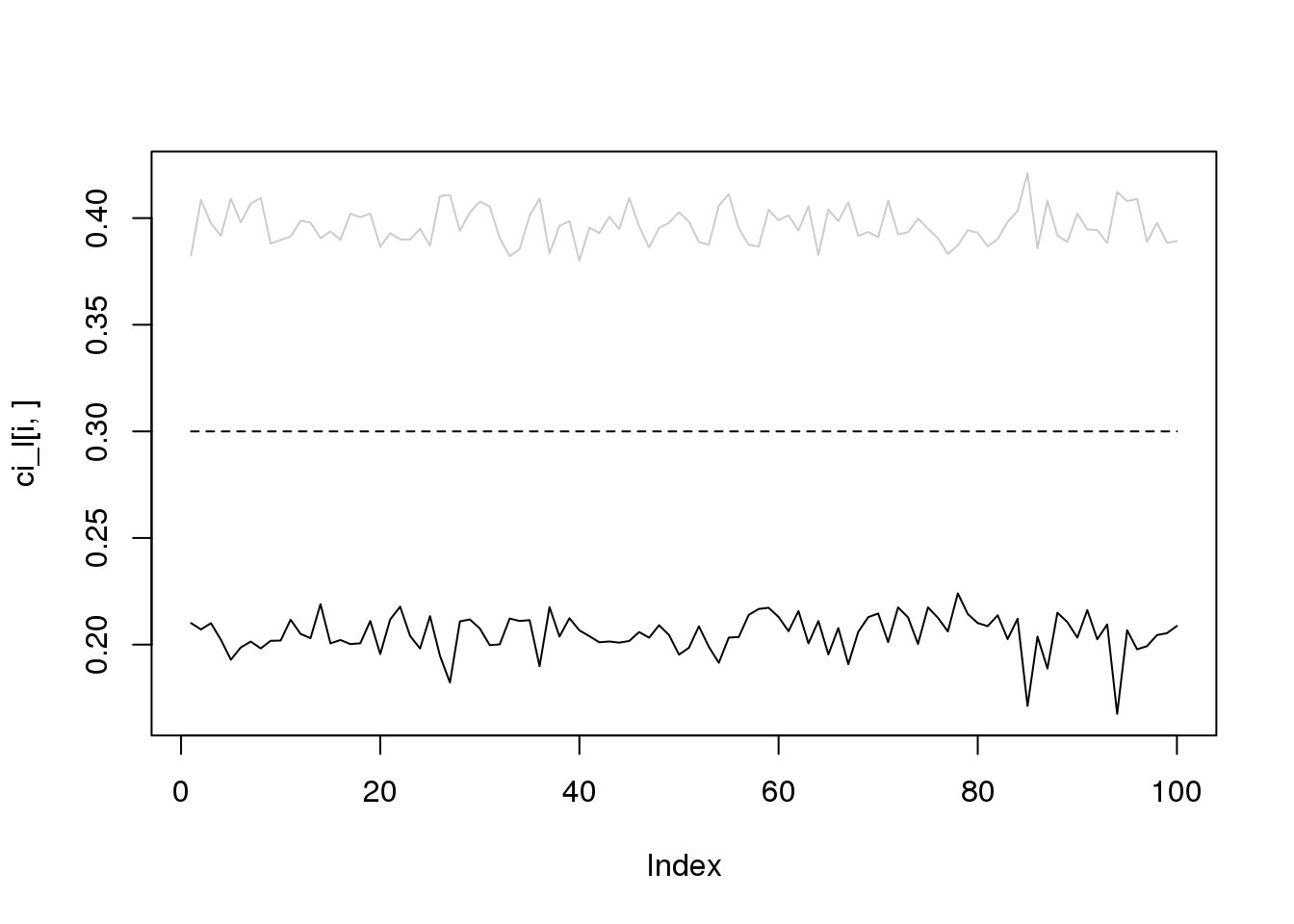
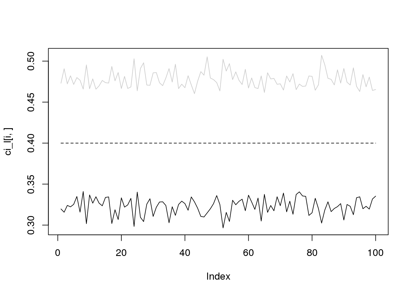
for(i in 1:4){
plot(ci_l[i,],type='l',ylim=range(c(ci_l[i,],ci_r[i,])))
lines(ci_r[i,],col='grey80')
lines(rep(i/10,100),lty = 2)
}
Another dataset:
XinT2D.eset = readRDS('data/deconv/XinT2Deset.rds')
XinT2D.eset
ExpressionSet (storageMode: lockedEnvironment)
assayData: 39849 features, 1492 samples
element names: exprs
protocolData: none
phenoData
sampleNames: Sample_1 Sample_2 ... Sample_1492 (1492 total)
varLabels: sampleID SubjectName ... Disease (5 total)
varMetadata: labelDescription
featureData: none
experimentData: use 'experimentData(object)'
Annotation: table(XinT2D.eset$cellType)
alpha  beta delta gamma
  886   472    49    85
# remove genes
rm.idx = which(rowSums((exprs(XinT2D.eset))!=0)<5)
rr = rowSums((exprs(XinT2D.eset)))
rm.idx2 = which(rr>=quantile(rr[-rm.idx],0.95))
rm.idx = unique(c(rm.idx,rm.idx2))
Theta = c()
S=c()
for(i in 1:4){
aa = rowSums(exprs(XinT2D.eset)[-rm.idx,which(XinT2D.eset$cellTypeID == i)])
Theta = cbind(Theta,aa/sum(aa))
S[i] = sum(aa)/length(which(XinT2D.eset$cellTypeID == i))
}
S=S/100
set.seed(12345)
# bulk data library size: 50*number of genes.
bulk_ls = 50*nrow(Theta)
# total number of cells in bulk data
bulk_ncell = 400
# cell proportions
bulk_beta = c(1,2,3,4)
bulk_beta = bulk_beta/sum(bulk_beta)
# bulk data gene relative expression.
bulk_X = bulk_ncell*Theta%*%diag(S)%*%bulk_beta
bulk_theta = bulk_X/sum(bulk_X)
ref_ncell = 100
ref_X = Theta%*%diag(S)*ref_ncell
w = rep(1,length(bulk_theta))
ci_l = c()
ci_r = c()
beta_est = c()
for(rep in 1:100){
Z = matrix(rpois(prod(dim(ref_X)),ref_X),ncol=ncol(ref_X))
y = rpois(length(bulk_theta),bulk_ls*bulk_theta)
#W = diag(w)
#beta_hat = solve(t(Z)%*%W%*%Z - diag(colSums(W%*%Z)))%*%t(Z)%*%W%*%y
beta_hat = solve(t(Z)%*%Z - diag(colSums(Z)))%*%t(Z)%*%y
#beta_hat = solve(t(Z)%*%Z)%*%t(Z)%*%y
#beta_hat
#beta_hat/sum(beta_hat)
Q = 0
Sigma=0
for(i in 1:length(y)){
ag = Z[i,]%*%t(Z[i,])-diag(Z[i,])
Q = Q + ag
Delta = (ag%*%beta_hat-y[i]*Z[i,])
Sigma = Sigma + Delta%*%t(Delta)
}
Q = Q*2/length(y)
Sigma = Sigma*4/length(y)
K = ncol(Z)
J = matrix(nrow = ncol(Z),ncol=ncol(Z))
for(i in 1:K){
for(j in 1:K){
if(i==j){
J[i,j] = sum(beta_hat)-beta_hat[i]
}else{
J[i,j] = -beta_hat[i]
}
}
}
asyV = J%*%solve(Q)%*%Sigma%*%solve(Q)%*%J
beta_est = rbind(beta_est,c(beta_hat))
ci_l = cbind(ci_l,beta_hat/sum(beta_hat)-2*sqrt(diag(asyV)/length(y)))
ci_r = cbind(ci_r,beta_hat/sum(beta_hat)+2*sqrt(diag(asyV)/length(y)))
}
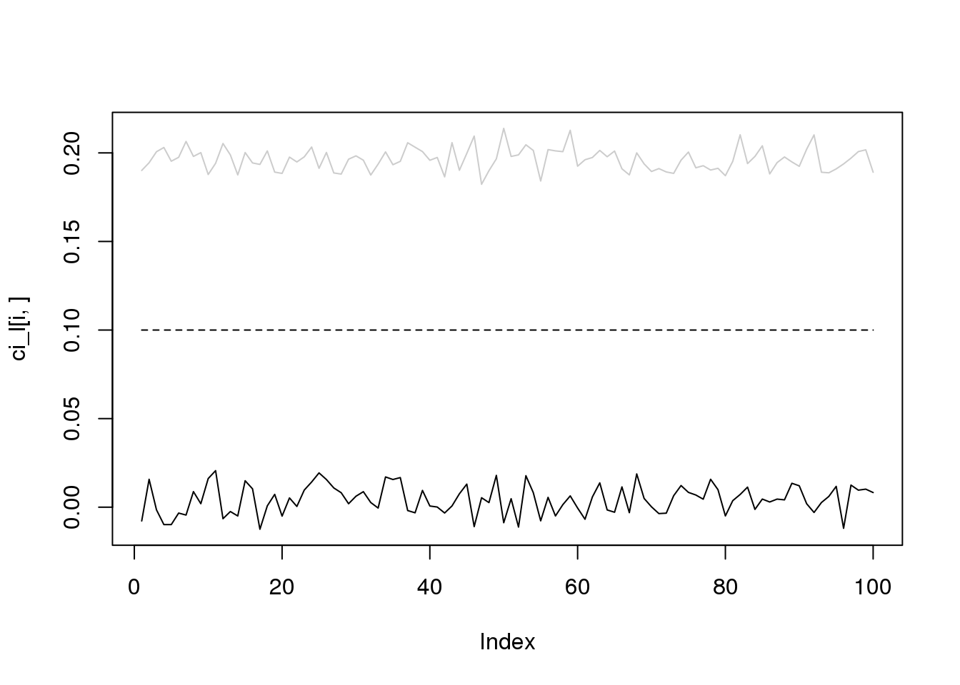
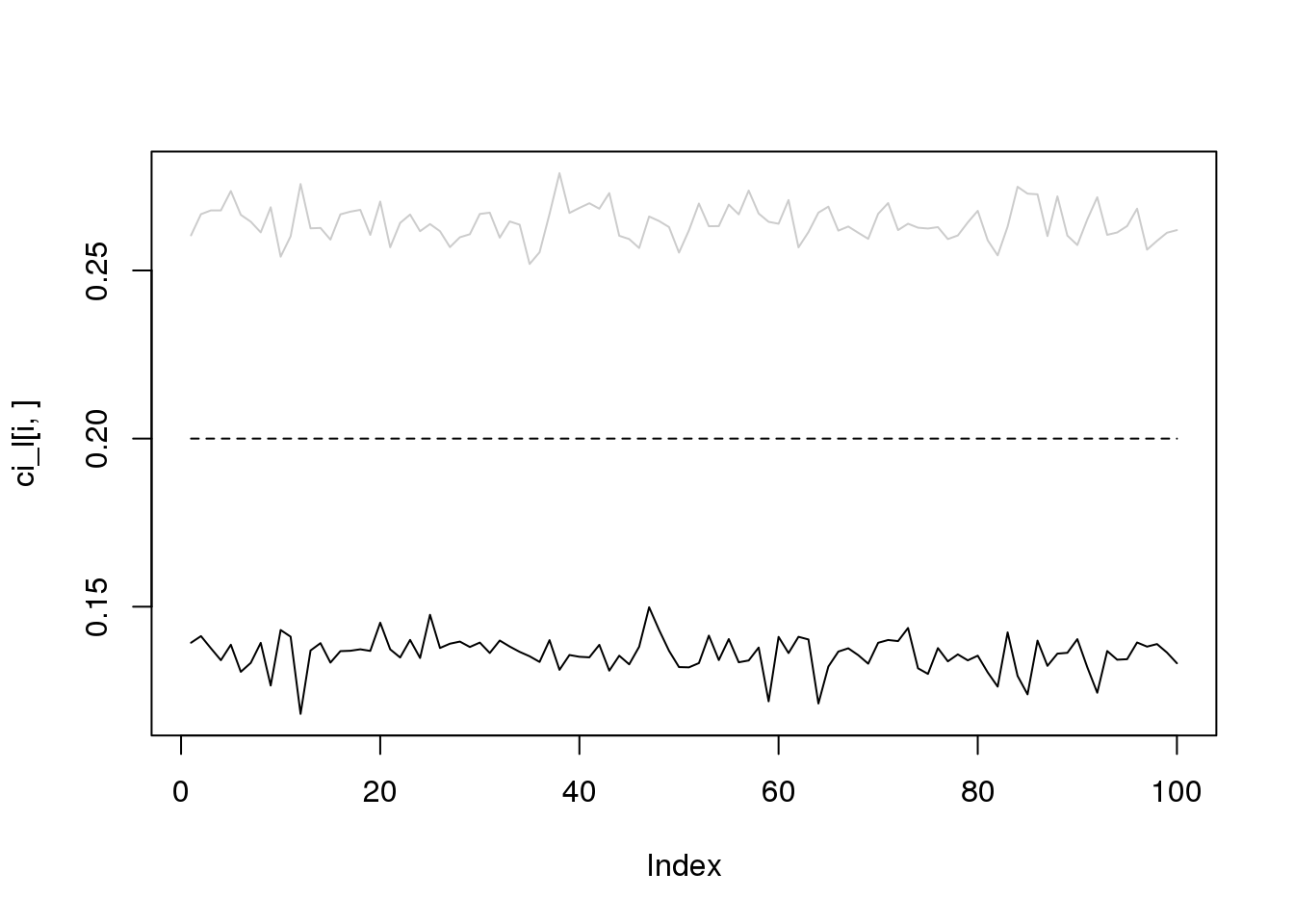
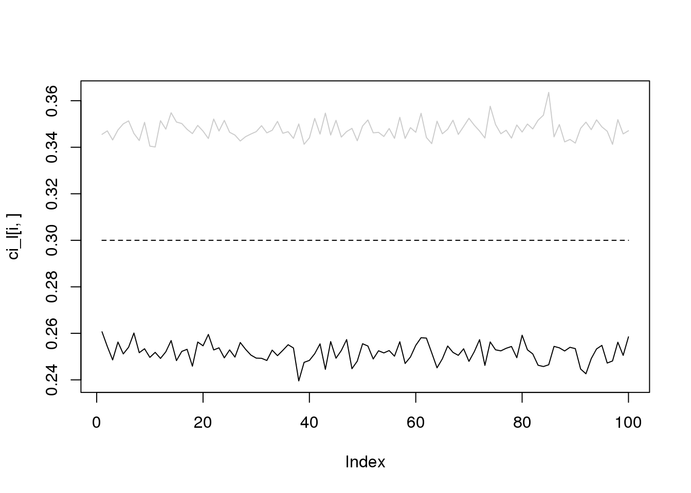
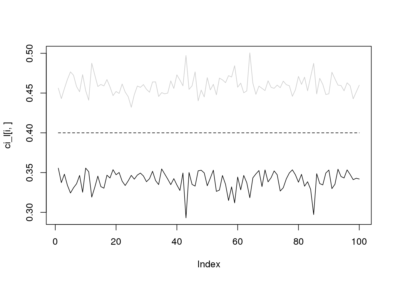
for(i in 1:4){
plot(ci_l[i,],type='l',ylim=range(c(ci_l[i,],ci_r[i,])))
lines(ci_r[i,],col='grey80')
lines(rep(i/10,100),lty = 2)
}
sessionInfo()R version 3.5.1 (2018-07-02)
Platform: x86_64-pc-linux-gnu (64-bit)
Running under: Scientific Linux 7.4 (Nitrogen)
Matrix products: default
BLAS/LAPACK: /software/openblas-0.2.19-el7-x86_64/lib/libopenblas_haswellp-r0.2.19.so
locale:
[1] LC_CTYPE=en_US.UTF-8 LC_NUMERIC=C
[3] LC_TIME=en_US.UTF-8 LC_COLLATE=en_US.UTF-8
[5] LC_MONETARY=en_US.UTF-8 LC_MESSAGES=en_US.UTF-8
[7] LC_PAPER=en_US.UTF-8 LC_NAME=C
[9] LC_ADDRESS=C LC_TELEPHONE=C
[11] LC_MEASUREMENT=en_US.UTF-8 LC_IDENTIFICATION=C
attached base packages:
[1] parallel stats graphics grDevices utils datasets methods
[8] base
other attached packages:
[1] Biobase_2.42.0 BiocGenerics_0.28.0
loaded via a namespace (and not attached):
[1] workflowr_1.6.0 Rcpp_1.0.2 digest_0.6.18 later_0.7.5
[5] rprojroot_1.3-2 R6_2.3.0 backports_1.1.2 git2r_0.26.1
[9] magrittr_1.5 evaluate_0.12 stringi_1.2.4 fs_1.3.1
[13] promises_1.0.1 whisker_0.3-2 rmarkdown_1.10 tools_3.5.1
[17] stringr_1.3.1 glue_1.3.0 httpuv_1.4.5 yaml_2.2.0
[21] compiler_3.5.1 htmltools_0.3.6 knitr_1.20