Aggregated Data Products for FACE-IT
Robert Schlegel & Jean-Pierre Gattuso
2021-09-28
Last updated: 2021-09-28
Checks: 6 1
Knit directory: WP1/
This reproducible R Markdown analysis was created with workflowr (version 1.6.2). The Checks tab describes the reproducibility checks that were applied when the results were created. The Past versions tab lists the development history.
The R Markdown is untracked by Git. To know which version of the R Markdown file created these results, you’ll want to first commit it to the Git repo. If you’re still working on the analysis, you can ignore this warning. When you’re finished, you can run wflow_publish to commit the R Markdown file and build the HTML.
Great job! The global environment was empty. Objects defined in the global environment can affect the analysis in your R Markdown file in unknown ways. For reproduciblity it’s best to always run the code in an empty environment.
The command set.seed(20210216) was run prior to running the code in the R Markdown file. Setting a seed ensures that any results that rely on randomness, e.g. subsampling or permutations, are reproducible.
Great job! Recording the operating system, R version, and package versions is critical for reproducibility.
Nice! There were no cached chunks for this analysis, so you can be confident that you successfully produced the results during this run.
Great job! Using relative paths to the files within your workflowr project makes it easier to run your code on other machines.
Great! You are using Git for version control. Tracking code development and connecting the code version to the results is critical for reproducibility.
The results in this page were generated with repository version 5786d9e. See the Past versions tab to see a history of the changes made to the R Markdown and HTML files.
Note that you need to be careful to ensure that all relevant files for the analysis have been committed to Git prior to generating the results (you can use wflow_publish or wflow_git_commit). workflowr only checks the R Markdown file, but you know if there are other scripts or data files that it depends on. Below is the status of the Git repository when the results were generated:
Ignored files:
    Ignored:    .Rhistory
    Ignored:    .Rproj.user/
    Ignored:    code/ny-alesund_cc_pf_rws.R
    Ignored:    data/model/
    Ignored:    data/pg_data/
    Ignored:    metadata/pangaea_parameters.tab

Untracked files:
    Untracked:  analysis/2021_analysis.Rmd
    Untracked:  code/FACE_IT_2021.R

Unstaged changes:
    Modified:   analysis/2021_summary.Rmd
    Modified:   analysis/_site.yml
    Modified:   code/functions.R
    Deleted:    talks/2021_analysis.Rmd
    Deleted:    talks/2021_analysis.html
    Deleted:    talks/2021_summary.Rmd
    Deleted:    talks/2021_summary.html
    Deleted:    talks/FACE_IT_2021.R
    Deleted:    talks/figures/is_fig_1.png
    Deleted:    talks/figures/kong_fig_1.png
    Deleted:    talks/figures/map_isfjorden.png
Note that any generated files, e.g. HTML, png, CSS, etc., are not included in this status report because it is ok for generated content to have uncommitted changes.
There are no past versions. Publish this analysis with wflow_publish() to start tracking its development.

[Abstract. Not for inclusion in final talk]
Multiple key drivers of change for Arctic socio-ecological fjord and adjacent coastal systems were identified at the outset of the FACE-IT project. The available data products that contain these key drivers were indexed in a meta-database as part of WP1. In addition to documenting where the relevant data are, how to access them, and which drivers they contain, the available data have also been downloaded and aggregated into data products that are currently available to FACE-IT members. A quick overview of the key drivers is provided before introducing the meta-database and an overview of the data of interest. The talk is concluded with a demonstration of how the data aggregated for Isfjorden may be used for a range of investigations from physical, to biological, to social. The aggregated data products showcased in this talk are intended to be used by other FACE-IT members for their research as well as to be used for a review of change in the FACE-IT study sites.
Isfjorden data

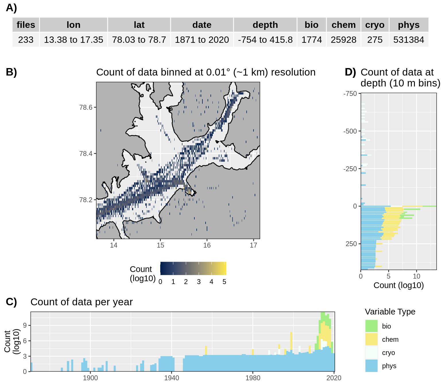
Figure 1: High level overview of the data available for Isfjorden. The acronyms for the variable groups seen throughout the figure are: bio = biology, chem = chemistry, cryo = cryosphere, phys = physical, soc = social (currently there are no social data for Isfjorden). A) Metadata showing the range of values available within the data. B) Spatial summary of data available per ~1 km grouping. Note that there are some important moorings outside of this bounding box that are included in the data counts. C) Temporal summary of available data. D) Summmary of data available by depth. Note that all of the data summaries are log10 transformed. For C) and D) the log10 transformation is applied before the data are stacked by category, which gives the impression that there are much more data are than there are.
Anthropogenic impacts in Isfjorden
- Keep in mind that this analysis is just an example to stimulate thought about real analyses
- These then are to be used for the review paper
- Have a specific focus on social science data because little effort has been done for social science so far
- For the analysis:
- Get the number of inhabitants of Longyearbyen over time and relate that to nutrient concentration
- Also want to look at relationships with ice cover and any sort of physical phenology
R version 4.1.1 (2021-08-10)
Platform: x86_64-pc-linux-gnu (64-bit)
Running under: Ubuntu 18.04.6 LTS

Matrix products: default
BLAS:   /usr/lib/x86_64-linux-gnu/blas/libblas.so.3.7.1
LAPACK: /usr/lib/x86_64-linux-gnu/lapack/liblapack.so.3.7.1

locale:
 [1] LC_CTYPE=en_GB.UTF-8       LC_NUMERIC=C
 [3] LC_TIME=fr_FR.UTF-8        LC_COLLATE=en_GB.UTF-8
 [5] LC_MONETARY=fr_FR.UTF-8    LC_MESSAGES=en_GB.UTF-8
 [7] LC_PAPER=fr_FR.UTF-8       LC_NAME=C
 [9] LC_ADDRESS=C               LC_TELEPHONE=C
[11] LC_MEASUREMENT=fr_FR.UTF-8 LC_IDENTIFICATION=C

attached base packages:
[1] parallel  grid      stats     graphics  grDevices utils     datasets
[8] methods   base

other attached packages:
 [1] doParallel_1.0.16  iterators_1.0.13   foreach_1.5.1      pangaear_1.1.0
 [5] sf_1.0-0           sp_1.4-5           RColorBrewer_1.1-2 ggOceanMaps_1.1.9
 [9] ggspatial_1.1.5    gtable_0.3.0       gridExtra_2.3      PCICt_0.5-4.1
[13] tidync_0.2.4       forcats_0.5.1      stringr_1.4.0      dplyr_1.0.6
[17] purrr_0.3.4        readr_1.4.0        tidyr_1.1.3        tibble_3.1.2
[21] ggplot2_3.3.3      tidyverse_1.3.1

loaded via a namespace (and not attached):
 [1] colorspace_2.0-1   ggsignif_0.6.2     ellipsis_0.3.2     class_7.3-19
 [5] rio_0.5.26         rprojroot_2.0.2    fs_1.5.0           rstudioapi_0.13
 [9] httpcode_0.3.0     proxy_0.4-26       ggpubr_0.4.0       farver_2.1.0
[13] fansi_0.5.0        lubridate_1.7.10   xml2_1.3.2         codetools_0.2-18
[17] ncdf4_1.17         knitr_1.33         jsonlite_1.7.2     workflowr_1.6.2
[21] broom_0.7.7        dbplyr_2.1.1       rgeos_0.5-5        oai_0.3.2
[25] hoardr_0.5.2       compiler_4.1.1     httr_1.4.2         backports_1.2.1
[29] assertthat_0.2.1   cli_2.5.0          later_1.2.0        htmltools_0.5.1.1
[33] tools_4.1.1        glue_1.4.2         rappdirs_0.3.3     Rcpp_1.0.6
[37] carData_3.0-4      cellranger_1.1.0   jquerylib_0.1.4    RNetCDF_2.4-2
[41] raster_3.4-10      vctrs_0.3.8        crul_1.1.0         xfun_0.23
[45] ps_1.6.0           openxlsx_4.2.3     rvest_1.0.0        lifecycle_1.0.0
[49] ncmeta_0.3.0       rstatix_0.7.0      scales_1.1.1       hms_1.1.0
[53] promises_1.2.0.1   yaml_2.2.1         curl_4.3.1         sass_0.4.0
[57] stringi_1.6.2      highr_0.9          e1071_1.7-7        zip_2.2.0
[61] rlang_0.4.11       pkgconfig_2.0.3    evaluate_0.14      lattice_0.20-44
[65] labeling_0.4.2     cowplot_1.1.1      tidyselect_1.1.1   processx_3.5.2
[69] plyr_1.8.6         magrittr_2.0.1     R6_2.5.0           generics_0.1.0
[73] DBI_1.1.1          foreign_0.8-81     pillar_1.6.1       haven_2.4.1
[77] withr_2.4.2        units_0.7-2        abind_1.4-5        modelr_0.1.8
[81] crayon_1.4.1       car_3.0-10         KernSmooth_2.23-20 utf8_1.2.1
[85] rmarkdown_2.8      sfheaders_0.4.0    readxl_1.3.1       data.table_1.14.0
[89] callr_3.7.0        git2r_0.28.0       reprex_2.0.0       digest_0.6.27
[93] classInt_0.4-3     httpuv_1.6.1       munsell_0.5.0      viridisLite_0.4.0
[97] bslib_0.2.5.1