Deep Visual Proteomics - snRNA-seq comparison
Florian Wuennemann
Last updated: 2024-03-21
Checks: 7 0
Knit directory: mi_spatialomics/
This reproducible R Markdown analysis was created with workflowr (version 1.7.1). The Checks tab describes the reproducibility checks that were applied when the results were created. The Past versions tab lists the development history.
Great! Since the R Markdown file has been committed to the Git repository, you know the exact version of the code that produced these results.
Great job! The global environment was empty. Objects defined in the global environment can affect the analysis in your R Markdown file in unknown ways. For reproduciblity it’s best to always run the code in an empty environment.
The command set.seed(20230612) was run prior to running
the code in the R Markdown file. Setting a seed ensures that any results
that rely on randomness, e.g. subsampling or permutations, are
reproducible.
Great job! Recording the operating system, R version, and package versions is critical for reproducibility.
Nice! There were no cached chunks for this analysis, so you can be confident that you successfully produced the results during this run.
Great job! Using relative paths to the files within your workflowr project makes it easier to run your code on other machines.
Great! You are using Git for version control. Tracking code development and connecting the code version to the results is critical for reproducibility.
The results in this page were generated with repository version e6213a5. See the Past versions tab to see a history of the changes made to the R Markdown and HTML files.
Note that you need to be careful to ensure that all relevant files for
the analysis have been committed to Git prior to generating the results
(you can use wflow_publish or
wflow_git_commit). workflowr only checks the R Markdown
file, but you know if there are other scripts or data files that it
depends on. Below is the status of the Git repository when the results
were generated:
Ignored files:
    Ignored:    .DS_Store
    Ignored:    .Rproj.user/
    Ignored:    analysis/.DS_Store
    Ignored:    analysis/deprecated/.DS_Store
    Ignored:    analysis/molecular_cartography_python/.DS_Store
    Ignored:    analysis/seqIF_python/.DS_Store
    Ignored:    analysis/seqIF_python/pixie/.DS_Store
    Ignored:    analysis/seqIF_python/pixie/cell_clustering/
    Ignored:    annotations/.DS_Store
    Ignored:    annotations/SeqIF/.DS_Store
    Ignored:    annotations/molkart/.DS_Store
    Ignored:    annotations/molkart/Figure1_regions/.DS_Store
    Ignored:    annotations/molkart/Supplementary_Figure4_regions/.DS_Store
    Ignored:    data/.DS_Store
    Ignored:    data/140623.calcagno_et_al.seurat_object.rds
    Ignored:    data/Calcagno2022_int_logNorm_annot.h5Seurat
    Ignored:    data/IC_03_IF_CCR2_CD68 cell numbers.xlsx
    Ignored:    data/Traditional_IF_absolute_cell_counts.csv
    Ignored:    data/Traditional_IF_relative_cell_counts.csv
    Ignored:    data/pixie.cell_table_size_normalized_cell_labels.csv
    Ignored:    data/results_cts_100.sqm
    Ignored:    data/seqIF_regions_annotations/
    Ignored:    data/seurat/
    Ignored:    omnipathr-log/
    Ignored:    output/.DS_Store
    Ignored:    output/mol_cart.harmony_object.h5Seurat
    Ignored:    output/molkart/
    Ignored:    output/proteomics/
    Ignored:    output/results_cts.lowres.125.sqm
    Ignored:    output/seqIF/
    Ignored:    pipeline_configs/.DS_Store
    Ignored:    plots/
    Ignored:    references/.DS_Store
    Ignored:    renv/.DS_Store
    Ignored:    renv/library/
    Ignored:    renv/staging/

Untracked files:
    Untracked:  analysis/deprecated/figures.supplementary_figureX.Rmd
    Untracked:  analysis/deprecated/figures.supplementary_figure_X.MistyR.Rmd

Unstaged changes:
    Deleted:    analysis/figures.supplementary_figureX.Rmd
    Deleted:    analysis/figures.supplementary_figure_X.MistyR.Rmd
    Deleted:    analysis/figures.supplementary_figure_X.proteomics_qc.Rmd
    Deleted:    figures/Figure_5.eps
    Deleted:    figures/Figure_5.pdf
    Deleted:    figures/Figure_5.png
    Deleted:    figures/Figure_5.svg
    Deleted:    figures/Supplementary_Figure_1_Molecular_Cartography_ROIs.png
    Deleted:    figures/Supplementary_figure_5.segmentation_metrics.poster.eps
    Modified:   figures/Supplementary_figure_X.proteomics.eps
    Modified:   figures/Supplementary_figure_X.proteomics.png
    Modified:   results_cts.lowres.125.sqm
Note that any generated files, e.g. HTML, png, CSS, etc., are not included in this status report because it is ok for generated content to have uncommitted changes.
These are the previous versions of the repository in which changes were
made to the R Markdown
(analysis/proteomics.scRNAseq_comparison.Rmd) and HTML
(docs/proteomics.scRNAseq_comparison.html) files. If you’ve
configured a remote Git repository (see ?wflow_git_remote),
click on the hyperlinks in the table below to view the files as they
were in that past version.
| File | Version | Author | Date | Message |
|---|---|---|---|---|
| Rmd | 56559c7 | FloWuenne | 2024-03-21 | Cleaned up repository. |
| Rmd | f35df9d | FloWuenne | 2024-03-02 | Updated figures for proteomic results. |
| html | 2dcd178 | FloWuenne | 2023-12-06 | wflow_publish("*") |
| Rmd | 5dee03d | FloWuenne | 2023-09-04 | Latest code update. |
| html | 5dee03d | FloWuenne | 2023-09-04 | Latest code update. |
| html | 67e546d | FloWuenne | 2023-07-23 | Build site. |
| Rmd | ed31d81 | FloWuenne | 2023-07-02 | Finalized proteomics analysis. |
| html | ed31d81 | FloWuenne | 2023-07-02 | Finalized proteomics analysis. |
| html | c1395e6 | FloWuenne | 2023-06-20 | Build site. |
| Rmd | 236130c | FloWuenne | 2023-06-20 | Updating proteomic analysis. |
| html | 236130c | FloWuenne | 2023-06-20 | Updating proteomic analysis. |
Introduction
Load data
We reprocessed the data from Calcagno et al, using the original cell-type annotations from the paper and will load this dataset as a seurat object.
## Load reprocessed Calcagno et al seurat object
calcagno_et_al <- LoadH5Seurat("./data/Calcagno2022_int_logNorm_annot.h5Seurat")
Validating h5Seurat fileInitializing RNA with dataAdding counts for RNAAdding miscellaneous information for RNAInitializing integrated with dataAdding scale.data for integratedAdding variable feature information for integratedAdding miscellaneous information for integratedAdding reduction pcaAdding cell embeddings for pcaAdding feature loadings for pcaAdding miscellaneous information for pcaAdding reduction umapAdding cell embeddings for umapAdding miscellaneous information for umapAdding graph integrated_nnAdding graph integrated_snnAdding command informationAdding cell-level metadataAdding miscellaneous informationAdding tool-specific resultsAdding data that was not associated with an assayWarning: Adding a command log without an assay associated with it## Get only control cells for marker calculation
calcagno_et_al_ds <- subset(calcagno_et_al,time == "D0")
calcagno_et_al_d1 <- subset(calcagno_et_al,time == "D1")Let’s check the UMAP embedding from our reprocessed object.
## UMAP plot
DimPlot(calcagno_et_al,label = TRUE) + theme(legend.position = "none")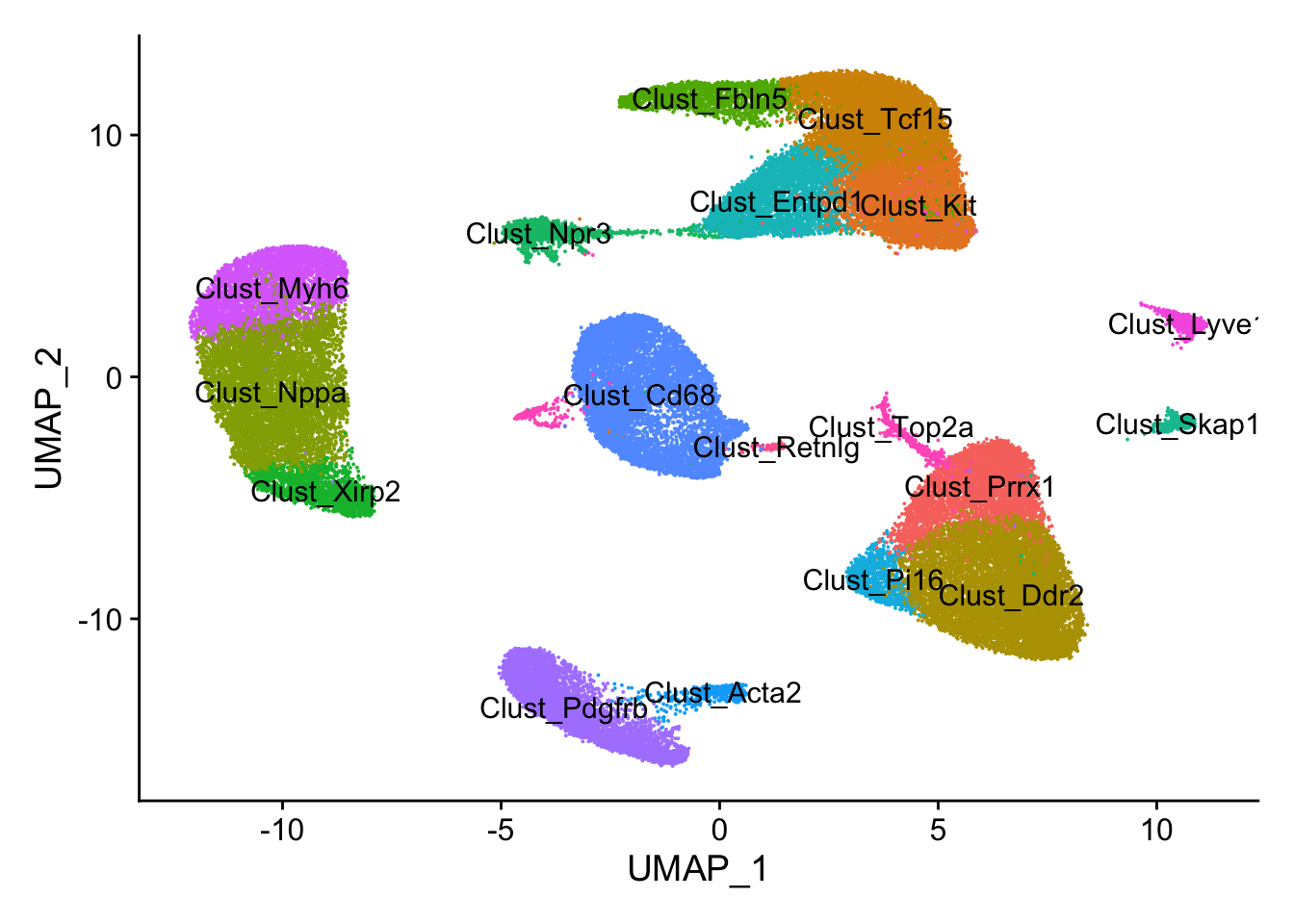
Next, let’s quickly verify, that Endocardial cells are expressing the proper markers before we compare them to our proteomic data.
plot_density(calcagno_et_al, features = "Npr3")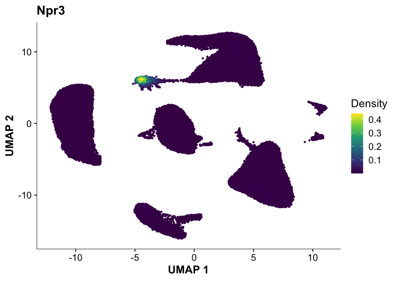
VlnPlot(calcagno_et_al, features = "Npr3")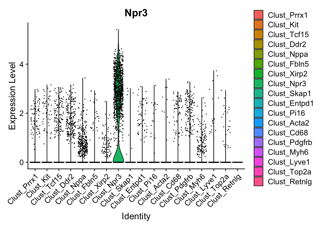
Expression of the endocardial specific marker Npr3 in this dataset fits with the original authors annotation, suggesting that we can use these endocardial single-cell signature to identify endocardial specific genes in our proteomics data.
Analyze cell-type specific proteins in proteomic data
We will use the snRNAseq data to identify proteins likely differentially expressed in endocardial cells. For this, we will first identify genes specifically expressed in endocardial cells.
Correlate pseudobulk snRNA-seq expression in endocardial cells with proteomic measurements
Let’s load the proteomic data now:
limma_res <- fread("./output/proteomics/proteomics.limma.full_statistics.tsv")

## Extract statistics for different contrasts
miiz_vs_control_signature <- subset(limma_res,analysis == "MI_IZ_vs_control")
miiz_vs_remote_signature <- subset(limma_res,analysis == "MI_IZ_vs_MI_remote")

## Load the normalized protein matrix as well
protein_mat <- fread(file = "./output/proteomics/proteomics.vsn_norm_proteins.tsv")
protein_mat_avg <- protein_mat %>%
  mutate(avg_control=rowMeans(.[ , c("control_r1","control_r2","control_r3")], na.rm=TRUE)) %>%
  mutate(avg_MI_IZ=rowMeans(.[ , c("MI_IZ_r1","MI_IZ_r2","MI_IZ_r3","MI_IZ_r4")], na.rm=TRUE)) %>%
  mutate(avg_MI_remote=rowMeans(.[ , c("MI_remote_r1","MI_remote_r2","MI_remote_r3","MI_remote_r4")], na.rm=TRUE)) %>%
  dplyr::select(gene,avg_control,avg_MI_IZ,avg_MI_remote)
## Calculate pseudobulk expression profiles for endocardial cells
endocard_seurat <- subset(calcagno_et_al, level_2 == "Endocardial")
sn_endo_bulk <- AverageExpression(endocard_seurat, group.by = c("time"),slot= "data")Warning: The `slot` argument of `AverageExpression()` is deprecated as of Seurat 5.0.0.
ℹ Please use the `layer` argument instead.
ℹ The deprecated feature was likely used in the Seurat package.
Please report the issue at <https://github.com/satijalab/seurat/issues>.
This warning is displayed once every 8 hours.
Call `lifecycle::last_lifecycle_warnings()` to see where this warning was
generated.As of Seurat v5, we recommend using AggregateExpression to perform pseudo-bulk analysis.
First group.by variable `time` starts with a number, appending `g` to ensure valid variable names
This message is displayed once per session.sn_endo_bulk_df <- as.data.frame(sn_endo_bulk$RNA)
sn_endo_bulk_df$gene <- rownames(sn_endo_bulk_df)## Merge average protein expression values with average RNA expression
rna_protein_avg <- left_join(protein_mat_avg,sn_endo_bulk_df, by = "gene") %>%
drop_na()
corrplot_rna_protein <- ggplot(rna_protein_avg,aes(avg_control,D0, label = gene)) +
geom_point() +
geom_point(data = subset(rna_protein_avg, gene == "Vwf"),color = "red", size =3) +
labs(x = "Average protein expression (Control)",
y = "Average snRNA-seq expression Control)")
corrplot_rna_protein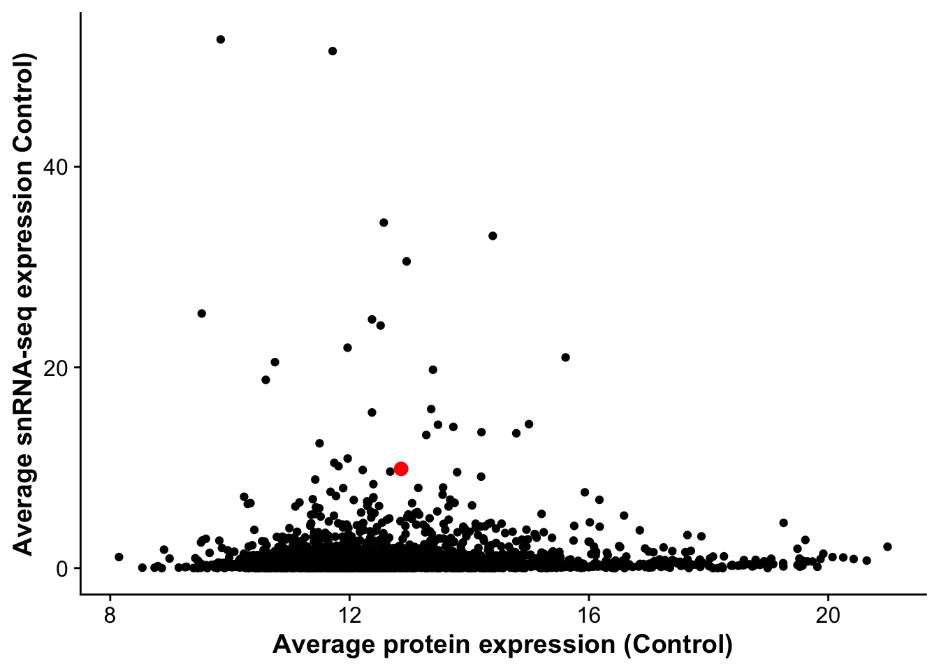
Calculate differentially expressed genes in endocardial cells in snRNA-seq
calcagno_et_al$cell_type_time <- paste(calcagno_et_al$level_2, calcagno_et_al$time,
    sep = "_")
Idents(calcagno_et_al) <- "cell_type_time"

endocard_de <- FindMarkers(calcagno_et_al,
                           ident.1 = "Endocardial_D1",
                           ident.2 = "Endocardial_D0",
                           min.diff.pct = 0.1,
                           logfc.threshold = 0,
                           verbose = FALSE)

colnames(endocard_de) <- gsub("\\.","_",colnames(endocard_de))
endocard_de <- endocard_de %>%
  mutate("gene" = rownames(endocard_de)) %>%
  mutate("pct_ratio" = pct_2 /pct_1,
         "pct_diff" = pct_2 -pct_1) %>%
  arrange(desc(avg_log2FC))
Get endocardial specific genes
To get an estimate of which genes are most specifically expressed in endocardialc ells in the snRNA-seq data, we will use the FindMarkers function from Seurat to get log-fold changes and p-values for the comparison of endocardial cells at day 0 to all other cells.
endo_marker <- FindMarkers(calcagno_et_al,ident.1 = "Endocardial_D0",
                           only.pos = TRUE)
endo_marker$gene <- rownames(endo_marker)
endo_marker <- endo_marker %>%
mutate("pct_diff" = pct.1 - pct.2) %>% # Only
mutate("pct_ratio" = pct.1 / pct.2) %>%
subset(pct.2 < 0.1) Compare endocardial specific genes with differentially expressed proteins (DEPs)
merged_protein_rna <- left_join(endo_marker,miiz_vs_remote_signature, by = "gene")

merged_protein_rna <- merged_protein_rna %>%
  mutate("label_gene" = if_else(gene %in% c("Vwf","Npr3"),gene,""))

endo_proteomic_corr <- ggplot(merged_protein_rna,aes(avg_log2FC,logFC,
                              label = label_gene)) +
  geom_point(data =subset(merged_protein_rna,gene != "Vwf"), size =3, fill = "darkgrey", pch = 21) +
  geom_point(data = subset(merged_protein_rna,gene == "Vwf"),size = 4, fill = "red", pch = 21) +
  geom_point(data = subset(merged_protein_rna,gene == "Npr3"),size = 4, fill = "purple", pch = 21) +
  geom_label_repel() +
  labs(x = "Specificity for endocardial cells (snRNA-seq)",
       y = "Log-fold change MI_IZ vs control(proteomics)")

endo_proteomic_corr
Warning: Removed 3236 rows containing missing values (`geom_point()`).Warning: Removed 3236 rows containing missing values (`geom_label_repel()`).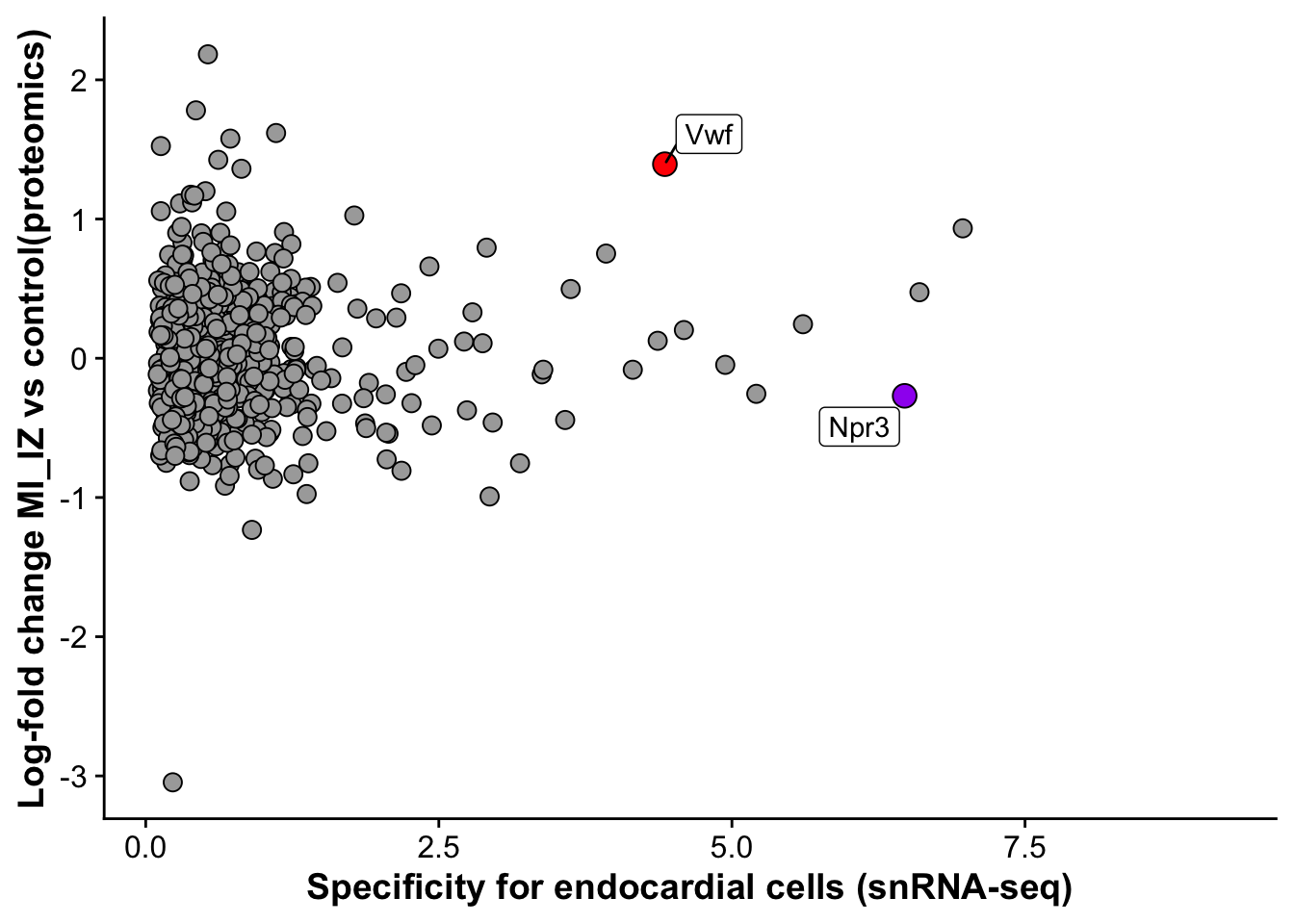
write.table(merged_protein_rna,
            file = "./output/proteomics/proteomics.snRNAseq_comp.tsv",
            sep = "\t",
            col.names = TRUE,
            row.names = FALSE,
            quote = FALSE)
sessionInfo()R version 4.3.1 (2023-06-16)
Platform: aarch64-apple-darwin20 (64-bit)
Running under: macOS Sonoma 14.1.2
Matrix products: default
BLAS: /Library/Frameworks/R.framework/Versions/4.3-arm64/Resources/lib/libRblas.0.dylib
LAPACK: /Library/Frameworks/R.framework/Versions/4.3-arm64/Resources/lib/libRlapack.dylib; LAPACK version 3.11.0
locale:
[1] en_US.UTF-8/en_US.UTF-8/en_US.UTF-8/C/en_US.UTF-8/en_US.UTF-8
time zone: Europe/Berlin
tzcode source: internal
attached base packages:
[1] stats graphics grDevices datasets utils methods base
other attached packages:
[1] RColorBrewer_1.1-3 ggsci_3.0.0 cowplot_1.1.2
[4] SeuratDisk_0.0.0.9021 plotly_4.10.4 ggrepel_0.9.5
[7] data.table_1.14.10 Nebulosa_1.12.0 patchwork_1.2.0
[10] Libra_1.7 nnls_1.5 here_1.0.1
[13] Seurat_5.0.1 SeuratObject_5.0.1 sp_2.1-2
[16] lubridate_1.9.3 forcats_1.0.0 stringr_1.5.1
[19] dplyr_1.1.4 purrr_1.0.2 readr_2.1.5
[22] tidyr_1.3.0 tibble_3.2.1 ggplot2_3.4.4
[25] tidyverse_2.0.0 workflowr_1.7.1
loaded via a namespace (and not attached):
[1] RcppAnnoy_0.0.21 splines_4.3.1
[3] later_1.3.2 bitops_1.0-7
[5] polyclip_1.10-6 fastDummies_1.7.3
[7] lifecycle_1.0.4 rprojroot_2.0.4
[9] hdf5r_1.3.8 globals_0.16.2
[11] processx_3.8.3 lattice_0.22-5
[13] MASS_7.3-60.0.1 magrittr_2.0.3
[15] limma_3.58.1 sass_0.4.8
[17] rmarkdown_2.25 jquerylib_0.1.4
[19] yaml_2.3.8 httpuv_1.6.14
[21] sctransform_0.4.1 spam_2.10-0
[23] spatstat.sparse_3.0-3 reticulate_1.34.0
[25] pbapply_1.7-2 abind_1.4-5
[27] zlibbioc_1.48.0 Rtsne_0.17
[29] GenomicRanges_1.54.1 presto_1.0.0
[31] BiocGenerics_0.48.1 RCurl_1.98-1.14
[33] pracma_2.4.4 git2r_0.33.0
[35] GenomeInfoDbData_1.2.11 IRanges_2.36.0
[37] S4Vectors_0.40.2 irlba_2.3.5.1
[39] listenv_0.9.0 spatstat.utils_3.0-4
[41] goftest_1.2-3 RSpectra_0.16-1
[43] spatstat.random_3.2-2 fitdistrplus_1.1-11
[45] parallelly_1.36.0 leiden_0.4.3.1
[47] codetools_0.2-19 DelayedArray_0.28.0
[49] tidyselect_1.2.0 farver_2.1.1
[51] matrixStats_1.2.0 stats4_4.3.1
[53] spatstat.explore_3.2-5 jsonlite_1.8.8
[55] ks_1.14.2 ellipsis_0.3.2
[57] progressr_0.14.0 ggridges_0.5.5
[59] survival_3.5-7 tools_4.3.1
[61] ica_1.0-3 Rcpp_1.0.12
[63] glue_1.7.0 gridExtra_2.3
[65] SparseArray_1.2.3 xfun_0.41
[67] MatrixGenerics_1.14.0 GenomeInfoDb_1.38.5
[69] withr_2.5.2 BiocManager_1.30.22
[71] fastmap_1.1.1 fansi_1.0.6
[73] callr_3.7.3 digest_0.6.34
[75] timechange_0.2.0 R6_2.5.1
[77] mime_0.12 colorspace_2.1-0
[79] scattermore_1.2 tensor_1.5
[81] spatstat.data_3.0-3 utf8_1.2.4
[83] generics_0.1.3 renv_1.0.3
[85] httr_1.4.7 htmlwidgets_1.6.4
[87] S4Arrays_1.2.0 whisker_0.4.1
[89] uwot_0.1.16 pkgconfig_2.0.3
[91] gtable_0.3.4 lmtest_0.9-40
[93] SingleCellExperiment_1.24.0 XVector_0.42.0
[95] htmltools_0.5.7 dotCall64_1.1-1
[97] scales_1.3.0 Biobase_2.62.0
[99] png_0.1-8 knitr_1.45
[101] rstudioapi_0.15.0 tzdb_0.4.0
[103] reshape2_1.4.4 nlme_3.1-164
[105] cachem_1.0.8 zoo_1.8-12
[107] KernSmooth_2.23-22 vipor_0.4.7
[109] parallel_4.3.1 miniUI_0.1.1.1
[111] ggrastr_1.0.2 pillar_1.9.0
[113] grid_4.3.1 vctrs_0.6.5
[115] RANN_2.6.1 promises_1.2.1
[117] xtable_1.8-4 cluster_2.1.6
[119] beeswarm_0.4.0 evaluate_0.23
[121] mvtnorm_1.2-4 cli_3.6.2
[123] compiler_4.3.1 rlang_1.1.3
[125] crayon_1.5.2 future.apply_1.11.1
[127] labeling_0.4.3 mclust_6.0.1
[129] ps_1.7.6 ggbeeswarm_0.7.2
[131] getPass_0.2-4 plyr_1.8.9
[133] fs_1.6.3 stringi_1.8.3
[135] viridisLite_0.4.2 deldir_2.0-2
[137] munsell_0.5.0 lazyeval_0.2.2
[139] spatstat.geom_3.2-7 Matrix_1.6-5
[141] RcppHNSW_0.5.0 hms_1.1.3
[143] bit64_4.0.5 future_1.33.1
[145] statmod_1.5.0 shiny_1.8.0
[147] highr_0.10 SummarizedExperiment_1.32.0
[149] ROCR_1.0-11 igraph_1.6.0
[151] bslib_0.6.1 bit_4.0.5