proteomics.bulk_de_analysis
FloWuenne
2023-06-14
Last updated: 2023-07-23
Checks: 7 0
Knit directory: mi_spatialomics/
This reproducible R Markdown analysis was created with workflowr (version 1.7.0). The Checks tab describes the reproducibility checks that were applied when the results were created. The Past versions tab lists the development history.
Great! Since the R Markdown file has been committed to the Git repository, you know the exact version of the code that produced these results.
Great job! The global environment was empty. Objects defined in the global environment can affect the analysis in your R Markdown file in unknown ways. For reproduciblity it’s best to always run the code in an empty environment.
The command set.seed(20230612) was run prior to running
the code in the R Markdown file. Setting a seed ensures that any results
that rely on randomness, e.g. subsampling or permutations, are
reproducible.
Great job! Recording the operating system, R version, and package versions is critical for reproducibility.
Nice! There were no cached chunks for this analysis, so you can be confident that you successfully produced the results during this run.
Great job! Using relative paths to the files within your workflowr project makes it easier to run your code on other machines.
Great! You are using Git for version control. Tracking code development and connecting the code version to the results is critical for reproducibility.
The results in this page were generated with repository version d6085a2. See the Past versions tab to see a history of the changes made to the R Markdown and HTML files.
Note that you need to be careful to ensure that all relevant files for
the analysis have been committed to Git prior to generating the results
(you can use wflow_publish or
wflow_git_commit). workflowr only checks the R Markdown
file, but you know if there are other scripts or data files that it
depends on. Below is the status of the Git repository when the results
were generated:
Ignored files:
    Ignored:    .DS_Store
    Ignored:    .Rhistory
    Ignored:    .Rproj.user/
    Ignored:    analysis/.DS_Store
    Ignored:    data/.DS_Store
    Ignored:    data/.Rapp.history
    Ignored:    data/140623.calcagno_et_al.seurat_object.rds
    Ignored:    omnipathr-log/
    Ignored:    plots/
    Ignored:    references/.DS_Store
    Ignored:    renv/.DS_Store
    Ignored:    renv/library/
    Ignored:    renv/staging/

Untracked files:
    Untracked:  data/cells_per_region.tsv
    Untracked:  figures/Supplementary_figure_5.segmentation_metrics.poster.eps

Unstaged changes:
    Modified:   analysis/figures.supplementary_Figure_3.Rmd
    Modified:   code/functions.R
    Modified:   figures/Figure_5.eps
    Modified:   figures/Figure_5.pdf
    Modified:   figures/Figure_5.png
    Modified:   figures/Figure_5.svg
    Modified:   figures/Supplementary_figure_5.segmentation_metrics.eps
    Modified:   figures/Supplementary_figure_5.segmentation_metrics.png
Note that any generated files, e.g. HTML, png, CSS, etc., are not included in this status report because it is ok for generated content to have uncommitted changes.
These are the previous versions of the repository in which changes were
made to the R Markdown
(analysis/proteomics.bulk_de_analysis.Rmd) and HTML
(docs/proteomics.bulk_de_analysis.html) files. If you’ve
configured a remote Git repository (see ?wflow_git_remote),
click on the hyperlinks in the table below to view the files as they
were in that past version.
| File | Version | Author | Date | Message |
|---|---|---|---|---|
| Rmd | ed31d81 | FloWuenne | 2023-07-02 | Finalized proteomics analysis. |
| html | ed31d81 | FloWuenne | 2023-07-02 | Finalized proteomics analysis. |
| html | c1395e6 | FloWuenne | 2023-06-20 | Build site. |
| Rmd | 236130c | FloWuenne | 2023-06-20 | Updating proteomic analysis. |
| html | 236130c | FloWuenne | 2023-06-20 | Updating proteomic analysis. |
library(data.table)
library(tidyverse)
── Attaching core tidyverse packages ──────────────────────── tidyverse 2.0.0 ──
✔ dplyr 1.1.2 ✔ readr 2.1.4
✔ forcats 1.0.0 ✔ stringr 1.5.0
✔ ggplot2 3.4.2 ✔ tibble 3.2.1
✔ lubridate 1.9.2 ✔ tidyr 1.3.0
✔ purrr 1.0.1
── Conflicts ────────────────────────────────────────── tidyverse_conflicts() ──
✖ dplyr::between() masks data.table::between()
✖ dplyr::filter() masks stats::filter()
✖ dplyr::first() masks data.table::first()
✖ lubridate::hour() masks data.table::hour()
✖ lubridate::isoweek() masks data.table::isoweek()
✖ dplyr::lag() masks stats::lag()
✖ dplyr::last() masks data.table::last()
✖ lubridate::mday() masks data.table::mday()
✖ lubridate::minute() masks data.table::minute()
✖ lubridate::month() masks data.table::month()
✖ lubridate::quarter() masks data.table::quarter()
✖ lubridate::second() masks data.table::second()
✖ purrr::transpose() masks data.table::transpose()
✖ lubridate::wday() masks data.table::wday()
✖ lubridate::week() masks data.table::week()
✖ lubridate::yday() masks data.table::yday()
✖ lubridate::year() masks data.table::year()
ℹ Use the conflicted package (<http://conflicted.r-lib.org/>) to force all conflicts to become errorslibrary(factoextra)Welcome! Want to learn more? See two factoextra-related books at https://goo.gl/ve3WBalibrary(ggsci)
library(cowplot)
Attaching package: 'cowplot'

The following object is masked from 'package:lubridate':

stamplibrary(here)here() starts at /Users/florian_wuennemann/1_Projects/MI_project/mi_spatialomicslibrary(proDA)
library(limma)
library(dplyr)
library(tibble)
library(tidyr)
library(ggplot2)
library(pheatmap)
library(ggrepel)
library(eulerr)
library(plotly)
Attaching package: 'plotly'

The following object is masked from 'package:ggplot2':

    last_plot

The following object is masked from 'package:stats':

    filter

The following object is masked from 'package:graphics':

layoutlibrary(vsn)Loading required package: Biobase
Loading required package: BiocGenerics
Attaching package: 'BiocGenerics'
The following object is masked from 'package:limma':
plotMA
The following objects are masked from 'package:lubridate':
intersect, setdiff, union
The following objects are masked from 'package:dplyr':
combine, intersect, setdiff, union
The following objects are masked from 'package:stats':
IQR, mad, sd, var, xtabs
The following objects are masked from 'package:base':
anyDuplicated, aperm, append, as.data.frame, basename, cbind,
colnames, dirname, do.call, duplicated, eval, evalq, Filter, Find,
get, grep, grepl, intersect, is.unsorted, lapply, Map, mapply,
match, mget, order, paste, pmax, pmax.int, pmin, pmin.int,
Position, rank, rbind, Reduce, rownames, sapply, setdiff, sort,
table, tapply, union, unique, unsplit, which.max, which.min
Welcome to Bioconductor
Vignettes contain introductory material; view with
'browseVignettes()'. To cite Bioconductor, see
'citation("Biobase")', and for packages 'citation("pkgname")'.library(limma)
source(here("./code/functions.R"))Introduction
Here we will perform an analysis to detect differentially expressed proteins (DEPs) between the healthy control endocardial layer (control), the endocardial layer adjacent to the infarct at 1 day post infarction (MI_IZ) and the endocardial layer that is remote to the infarct from the same heart as the MI_IZ.
We will compare two different methods to perform differential expresssion, proDA, which models missing values in it’s statistical model and limma, which uses linear models and can handle missing values.
Load data
First, let’s load the filtered protein table from the previous step Filter proteomic data.
## Import imputed protein table (our "bulk" data)
clean_proteins <- fread(file = "./output/proteomics.filtered_proteins.tsv")
## First we format the protein matrix for DEP analysis
## Remove duplicates
dups <- clean_proteins[duplicated(clean_proteins$Genes),"Genes"]
clean_proteins_nd <- subset(clean_proteins,!Genes %in% unique(dups$Genes))
## Store gene and protein IDs
protein_ids <- clean_proteins_nd$Protein_Ids
gene_mapping <- clean_proteins_nd %>%
select(Protein_Ids,Genes)
## Remove annotation columns
abundance_matrix <- clean_proteins_nd %>%
select(-c(Protein_Group,Protein_Ids,Protein_Names,Genes))
rownames(abundance_matrix) <- protein_idsNormalize data
We use the vsn package to normalize our expression data. The vsn normalization function takes non-logged values as input.
## Use vsn normalization on the raw values (non log-transformed)
vsnMatrix <- normalizeVSN(abundance_matrix)
meanSdPlot(vsnMatrix)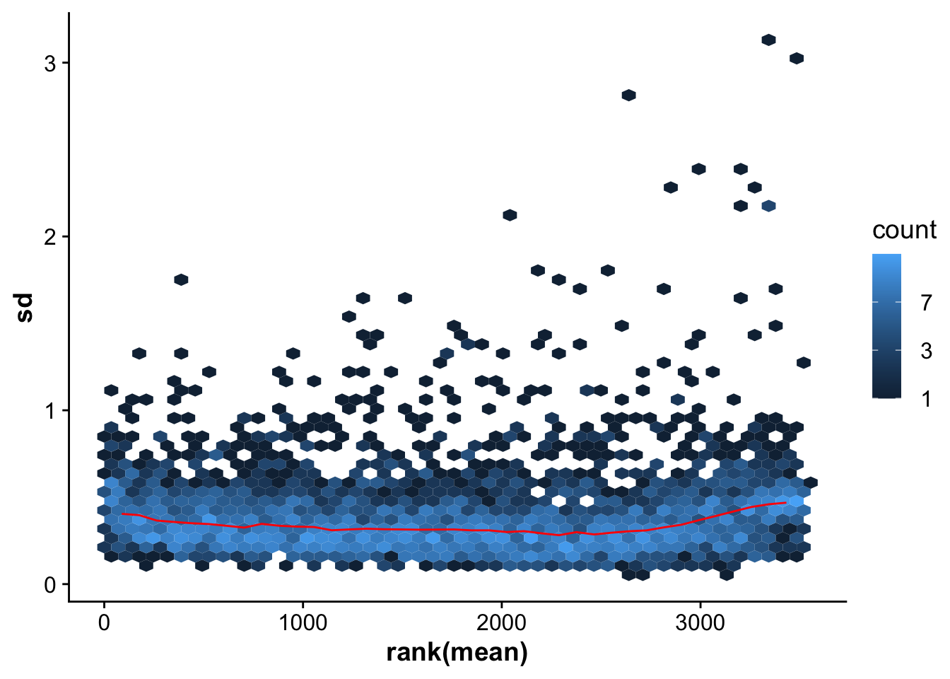
| Version | Author | Date |
|---|---|---|
| ed31d81 | FloWuenne | 2023-07-02 |
## Save vsn normalized protein expression values
vsnMatrix_store <- as.data.frame(vsnMatrix)
vsnMatrix_store$gene <- gene_mapping$Genes
write.table(vsnMatrix_store,
            file = "./output/proteomics.vsn_norm_proteins.tsv",
            col.names = TRUE,
            row.names = FALSE,
            quote = FALSE)
Principal component analysis of proteomic samples
As a fist QC, we will do a principal component analysis (PCA) of the samples. Due to the strong perturbation effect of myocardial infarction, we expect to find samples distributed by group (control, MI_remote, MI_IZ) in the first principle component.
abundance_matrix_pc <- as.data.frame(vsnMatrix) %>%
  drop_na()

## Calculate principal components and plot the firs two PCs
res.pca <- prcomp(t(abundance_matrix_pc), scale = TRUE)
fviz_eig(res.pca, addlabels = TRUE)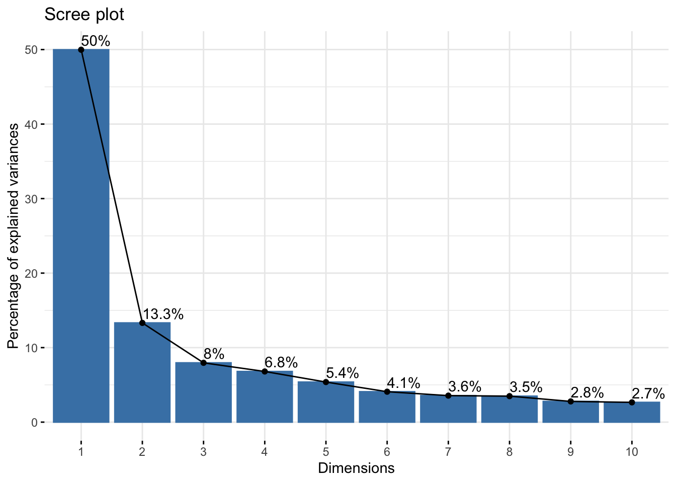
pcs <- as.data.frame(res.pca$x)
pcs$sample <- colnames(abundance_matrix_pc)
pcs <- pcs %>%
  mutate("group" = if_else(grepl("control",sample),"control",
                          if_else(grepl("MI_IZ",sample),"MI_IZ","MI_remote"))
         )

## Set order of groups
pcs$group <- factor(pcs$group,
                    levels = c("control","MI_remote","MI_IZ"))

## Plot PCs
ggplot(pcs,aes(PC1,PC2, color = group, fill = group)) +
  geom_point(size = 5,pch = 21,color = "black") +
  scale_fill_manual(values = proteome_palette,
                    labels = c("Control","MI_remote","MI_IZ")) +
  labs(color = "Group") +
  guides(fill=guide_legend(title="Treatment group"))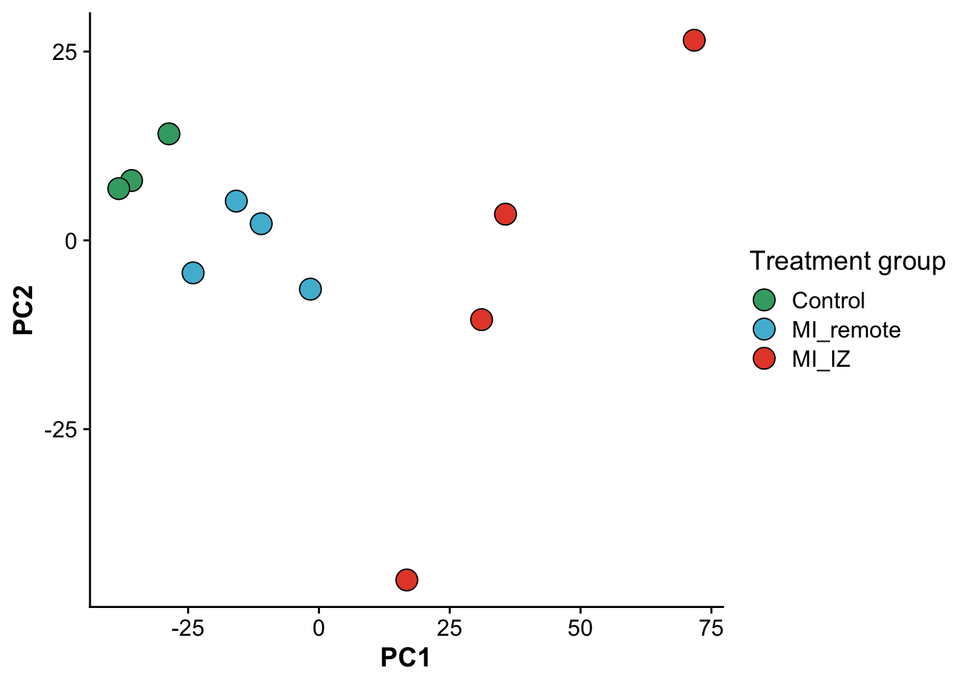
| Version | Author | Date |
|---|---|---|
| ed31d81 | FloWuenne | 2023-07-02 |
saveRDS(res.pca,
        file = "./output/proteomics.pca_res.rds")
As expected, samples separate in PC1, based on their group category, confirming that the strongest effect between samples is whether the heart experienced an infarct and the location of the endocardial cells relative to the infarct zone.
DEPs using limma
Let’s use limma to identif differentially expressed proteins
We will define a design matrix to perform differential expression testing in proDA.
design_matrix <- pcs %>%
  select(sample,group)

control_mi_cont <- c(0,0,0,1,1,1,1)
iz_remote_cont <- c(0,0,0,0,1,1,1,1)

## column numbers of different groups
control_idx <- c(1,2,3)
mi_iz_idx <- c(4,5,6,7)
mi_remote_idx <- c(8,9,10,11)
design <- model.matrix(~ 0 + design_matrix$group)
rownames(design) <- design_matrix$sample
colnames(design) <- gsub("design_matrix\\$groupMI_","",colnames(design))
colnames(design) <- gsub("design_matrix\\$group","",colnames(design))fit <- lmFit(vsnMatrix, design)Warning: Partial NA coefficients for 123 probe(s)contrast.matrix <- makeContrasts(MI_vs_Ctr = IZ - control,
remote_vs_Ctr = remote - control,
MI_vs_remote = IZ - remote,
levels = design)
fit_contrast <- contrasts.fit(fit, contrast.matrix)
fit_contrast <- eBayes(fit_contrast)
## MI_IZ vs control
limma_mi_ctr <- topTable(fit_contrast,
n=Inf, adjust.method = 'BH', coef= "MI_vs_Ctr",
sort.by = "none")
limma_mi_ctr$gene <- gene_mapping$Genes
limma_mi_ctr$protein_ids <- gene_mapping$Protein_Ids
limma_mi_ctr <- limma_mi_ctr %>%
arrange(adj.P.Val) %>%
mutate("pval" = P.Value,
"analysis" = "MI_IZ_vs_control")
## MI_remote vs MI_remote
limma_remote_ctr <- topTable(fit_contrast,
n=Inf, adjust.method = 'BH', coef= "remote_vs_Ctr",
sort.by = "none")
limma_remote_ctr$gene <- gene_mapping$Genes
limma_remote_ctr$protein_ids <- gene_mapping$Protein_Ids
limma_remote_ctr <- limma_remote_ctr %>%
arrange(adj.P.Val) %>%
mutate("pval" = P.Value,
"analysis" = "MI_remote_vs_control")
limma_remote_ctr$label_protein <- ""
## MI_IZ vs MI_remote
limma_mi_remote <- topTable(fit_contrast,
n=Inf, adjust.method = 'BH', coef= "MI_vs_remote",
sort.by = "none")
limma_mi_remote$gene <- gene_mapping$Genes
limma_mi_remote$protein_ids <- gene_mapping$Protein_Ids
limma_mi_remote <- limma_mi_remote %>%
arrange(adj.P.Val) %>%
mutate("pval" = P.Value,
"analysis" = "MI_IZ_vs_MI_remote")Let’s visualize the differential expression results using Volcano plots and highlighting the top protein hits per group.
Comparison of MI_IZ with control endocardial region
The first comparison we are interested in is comparing the remote zone from infarcted hearts with controls endocardium. This comparison will highlight programs upregulated mainly due to the systemic inflammatory response to myocardial infarction.
## Volcano plot of IZ_remote vs control
limma_mi_ctr$label_protein <- ""
volc_limma_remote_ctr <- plot_pretty_volcano(limma_mi_ctr,
                                      pt_size = 2,
                                      plot_title = "MI_IZ vs control",
                                      sig_thresh = 0.05,
                                      col_pos_logFC = "#E64B35FF",
                                      col_neg_logFC = "#3DA873FF")
ggplotly(volc_limma_remote_ctr)
## Plot two targets to check resultsComparison of MI_IZ with MI_remote endocardial region
## Volcano plot of IZ_remote vs control
limma_mi_remote$label_protein <- ""
volc_limma_IZ_remote <- plot_pretty_volcano(limma_mi_remote,
                                      pt_size = 2,
                                      plot_title = "MI_IZ vs MI_remote",
                                      sig_thresh = 0.05,
                                      col_pos_logFC = "#E64B35FF",
                                      col_neg_logFC = "#4DBBD5FF")
ggplotly(volc_limma_IZ_remote)
Save results
Let’s combine the results from the limma test into one big table and save it for later use.
limma_merged_stats <- rbind(limma_mi_ctr,limma_remote_ctr,limma_mi_remote)

write.table(limma_merged_stats,
            file = "./output/limma.full_statistics.tsv",
            sep = "\t",
            col.names = TRUE,
            row.names = FALSE,
            quote = FALSE)
Venn Diagram of DE genes
limma_mi_ctr_genes <- subset(limma_mi_ctr,adj.P.Val <= 0.05)$gene
limma_remote_ctr_genes <- subset(limma_remote_ctr,adj.P.Val <= 0.05)$gene
limma_mi_remote_genes <- subset(limma_mi_remote,adj.P.Val <= 0.05)$gene
limma_venn_vec <- limma_mi_ctr$gene
limma_venn_df <- data.frame("MI_control" = limma_venn_vec %in% limma_mi_ctr_genes,
                      "remote_control" = limma_venn_vec %in% limma_remote_ctr_genes,
                      "MI_IZ_MI_remote" = limma_venn_vec %in% limma_mi_remote_genes)
limma_venn_df$gene <- limma_venn_vec

## Plot the 3 group Venn diagram
plot(venn(limma_venn_df[,1:3]))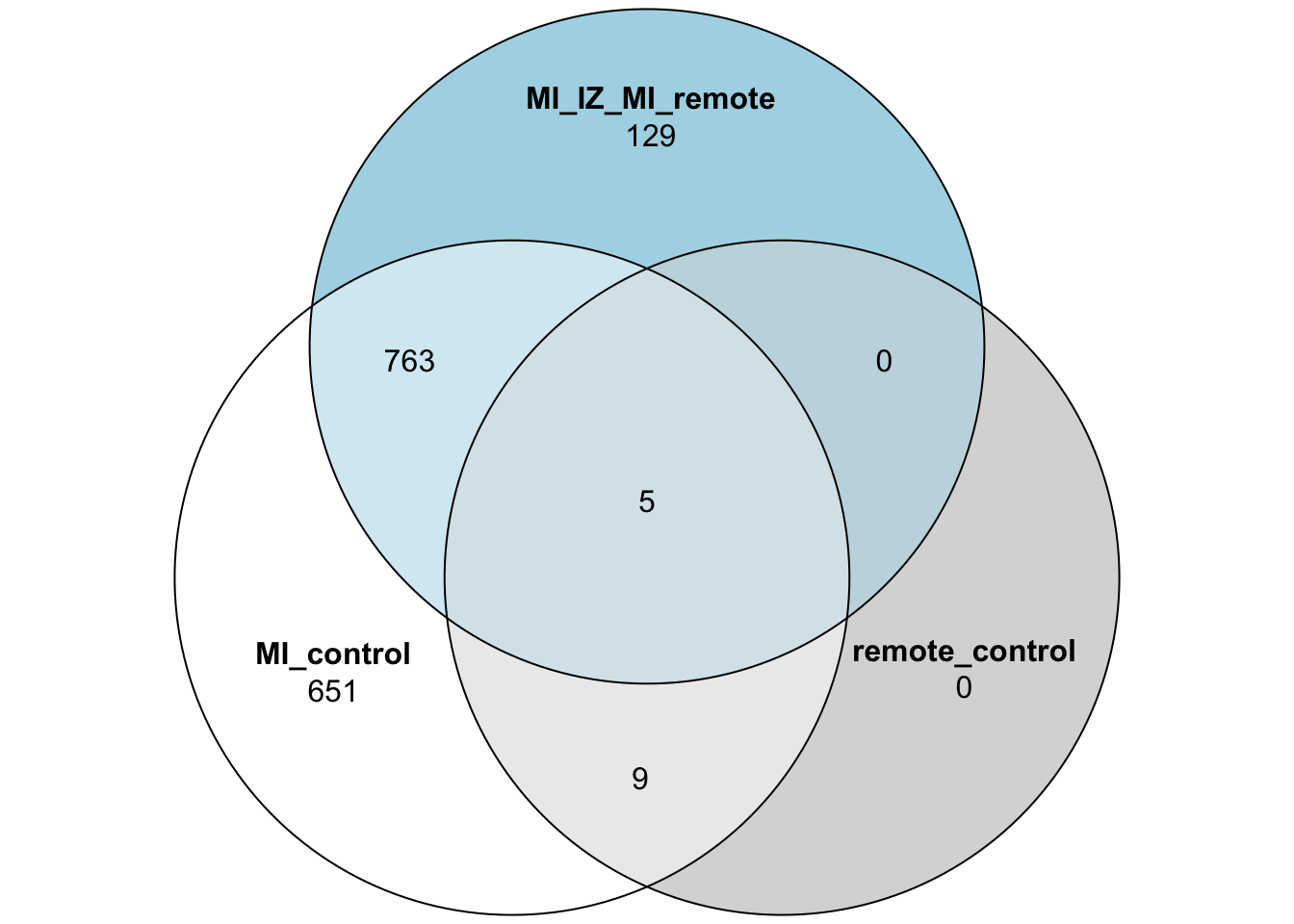
DEPs using proDA
Fit proDA full model and apply contrasts to compare to control
We will fit a model on the full vsn matrix and set the control group as the reference level, to compare MI_IZ and MI_remote to the control.
fit_full <- proDA(vsnMatrix,  design = ~ group,
             col_data = design_matrix, reference_level = "control")
Let’s now look at the approximate sample distance matrix based on the proDA model.
da <- dist_approx(fit_full)plot_mat <- as.matrix(da$mean)
pheatmap::pheatmap(plot_mat)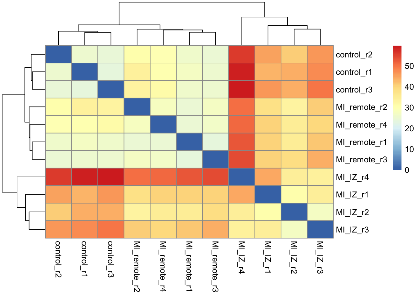
Now we will extract the test statistics for the different comparisons and visualize them using volcano plots.
MI_IZ vs control
test_res_miiz <- test_diff(fit_full, "groupMI_IZ", pval_adjust_method = "BH")
test_res_miiz$gene <- gene_mapping$Genes
test_res_miiz$protein_ids <- gene_mapping$Protein_Ids
test_res_miiz <- test_res_miiz %>%
  arrange(adj_pval) %>%
  mutate("logFC" = diff,
         "analysis" = "MI_IZ_vs_control")
test_res_miiz$label_protein <- ""

volc_test_miiz <- plot_pretty_volcano(test_res_miiz,
                                      pt_label = "gene", pt_size = 2,
                                      plot_title = "MI_IZ vs control",
                                      sig_thresh = 0.05,
                                      sig_col = "adj_pval")
ggplotly(volc_test_miiz)
MI_remote vs control
test_res_miremote <- test_diff(fit_full, "groupMI_remote", pval_adjust_method = "fdr")
test_res_miremote$gene <- gene_mapping$Genes
test_res_miremote$protein_ids <- gene_mapping$Protein_Ids
test_res_miremote <- test_res_miremote %>%
  arrange(adj_pval) %>%
  mutate("logFC" = diff,
         "analysis" = "MI_remote_vs_control")
test_res_miremote$label_protein <- ""

volc_test_miremote <- plot_pretty_volcano(test_res_miremote,
                                      pt_label = "gene", pt_size = 2,
                                      plot_title = "MI_remote vs control",
                                      sig_thresh = 0.05,
                                      sig_col = "adj_pval")
ggplotly(volc_test_miremote)
IZ vs remote
vsnMatrix_sub <- vsnMatrix[,c(mi_iz_idx,mi_remote_idx)]

fit_iz_remote <- proDA(vsnMatrix_sub, design = as.factor(c("MI_IZ","MI_IZ","MI_IZ","MI_IZ","MI_remote","MI_remote","MI_remote","MI_remote")))
test_res_iz_remote <- test_diff(fit_iz_remote, MI_IZ - MI_remote, pval_adjust_method = "fdr")
test_res_iz_remote$gene <- gene_mapping$Genes
test_res_iz_remote$protein_ids <- gene_mapping$Protein_Ids
test_res_iz_remote <- test_res_iz_remote %>%
arrange(adj_pval) %>%
mutate("logFC" = diff,
"analysis" = "MI_IZ_vs_MI_remote")
test_res_iz_remote$label_protein <- ""
volc_test_iz_remote <- plot_pretty_volcano(test_res_iz_remote,
pt_label = "gene", pt_size = 2,
plot_title = "MI_IZ vs remote",
sig_thresh = 0.05,
sig_col = "adj_pval")
ggplotly(volc_test_iz_remote)Merge results of proDA analysis
merged_stats <- rbind(test_res_miiz,test_res_miremote,test_res_iz_remote)Venn Diagram of DE genes
test_res_miiz_genes <- subset(test_res_miiz,adj_pval <= 0.05)$gene
test_res_miremote_genes <- subset(test_res_miremote,adj_pval <= 0.05)$gene
test_res_iz_remote_genes <- subset(test_res_iz_remote,adj_pval <= 0.05)$gene
proda_venn_vec <- test_res_miiz$gene
proda_venn_df <- data.frame("MI_control" = proda_venn_vec %in% test_res_miiz_genes,
                      "remote_control" = proda_venn_vec %in% test_res_miremote_genes,
                      "MI_IZ_MI_remote" = proda_venn_vec %in% test_res_iz_remote_genes)
proda_venn_df$gene <- proda_venn_vec

## Plot the 3 group Venn diagram
plot(venn(proda_venn_df[,1:3]))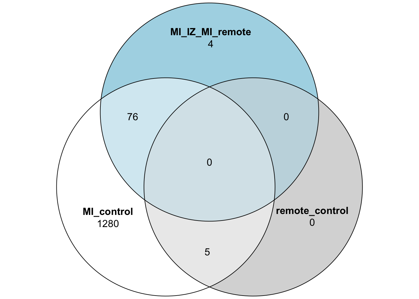
| Version | Author | Date |
|---|---|---|
| ed31d81 | FloWuenne | 2023-07-02 |
## get proteins that are deferentially expressed between MI vs control and MI_IZ and MI_remote
MI_IZ_proteins <- subset(proda_venn_df,MI_control == TRUE & remote_control == FALSE &  MI_IZ_MI_remote == TRUE)$gene

## Get proteins that are found differentially expressed between MI_IZ vs control as well as MI_IZ vs MI_remote. These proteins represent specific differences in MI_IZ layer due to inflammation
MI_induced_prots_IZ <- subset(proda_venn_df,MI_control == TRUE & remote_control == FALSE &  MI_IZ_MI_remote == TRUE)
MI_induced_prots_IZ <- subset(test_res_iz_remote,gene %in% MI_induced_prots_IZ$gene)
mi_iz_unique_genes <- subset(MI_induced_prots_IZ, adj_pval <= 0.05)
write.table(unique(mi_iz_unique_genes$gene),
file = "./output/mi_iz_specific_proteins.tsv",
col.names = FALSE,
row.names = FALSE,
quote = FALSE)Compare proDA with limma results
Finally, let’s compare the limma results to the proDA results for one comparison (MI_IZ vs control) to see how they differ.
merged_tests_mictr <- full_join(test_res_miiz,limma_mi_ctr, by = c("gene","protein_ids"))

merged_tstat <- ggplot(merged_tests_mictr,aes(t_statistic,t)) +
  geom_point() +
  geom_smooth() +
  labs(x = "proDA t-statistic",
       y = "limma t-statistic",
       title = "Comparison of t-statistics")
merged_tstat
`geom_smooth()` using method = 'gam' and formula = 'y ~ s(x, bs = "cs")'Warning: Removed 114 rows containing non-finite values (`stat_smooth()`).Warning: Removed 114 rows containing missing values (`geom_point()`).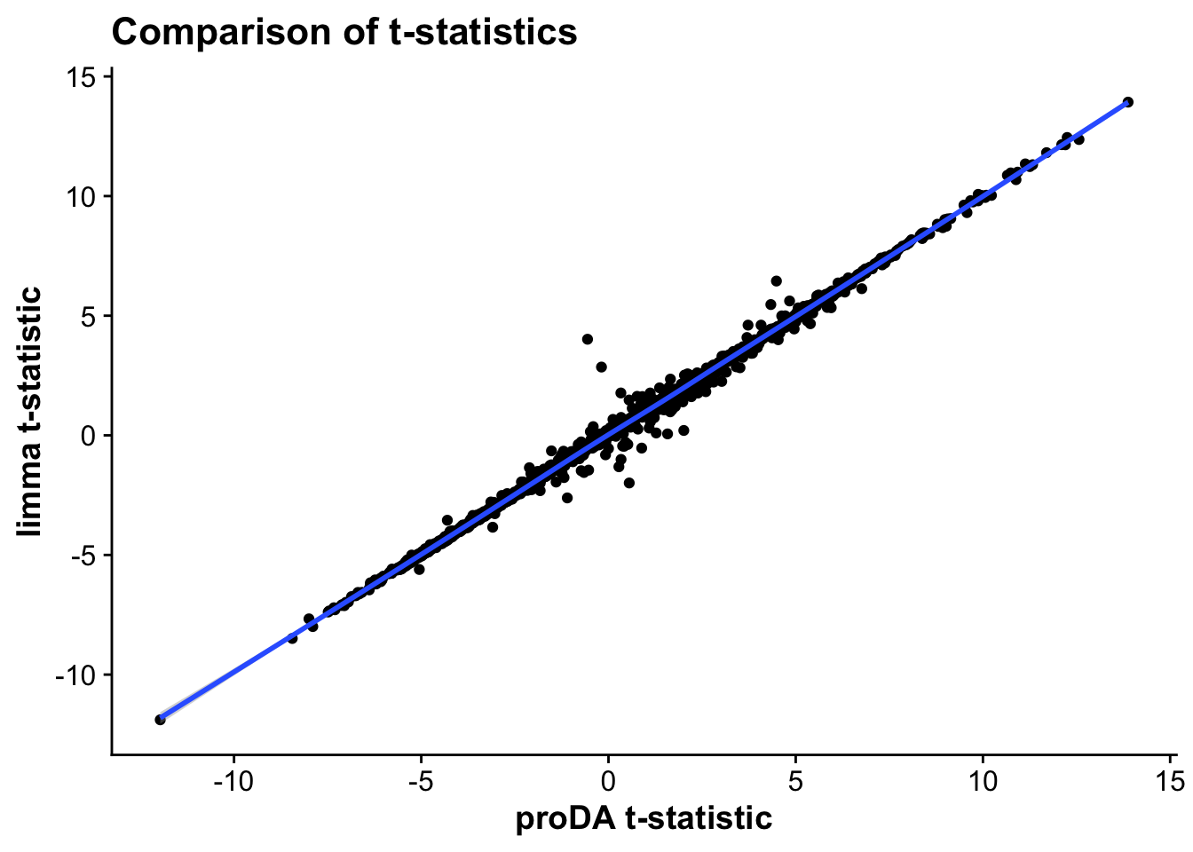
| Version | Author | Date |
|---|---|---|
| ed31d81 | FloWuenne | 2023-07-02 |
merged_diffs_mictr <- ggplot(merged_tests_mictr,aes(diff,logFC.y,label = gene)) +
  geom_point() +
  geom_smooth() +
  labs(x = "proDA diff",
       y = "limma logFC",
       title = "Comparison of diff and log-fold changes")

merged_abundance_mictr <- ggplot(merged_tests_mictr,aes(avg_abundance,AveExpr,
                                            label = gene)) +
  geom_point() +
  geom_smooth() +
  labs(x = "proDA avg_abundance",
       y = "limma AveExpr",
       title = "Comparison of average abundance per protein")
merged_abundance_mictr
`geom_smooth()` using method = 'gam' and formula = 'y ~ s(x, bs = "cs")'Warning: The following aesthetics were dropped during statistical transformation: label
ℹ This can happen when ggplot fails to infer the correct grouping structure in
the data.
ℹ Did you forget to specify a `group` aesthetic or to convert a numerical
variable into a factor?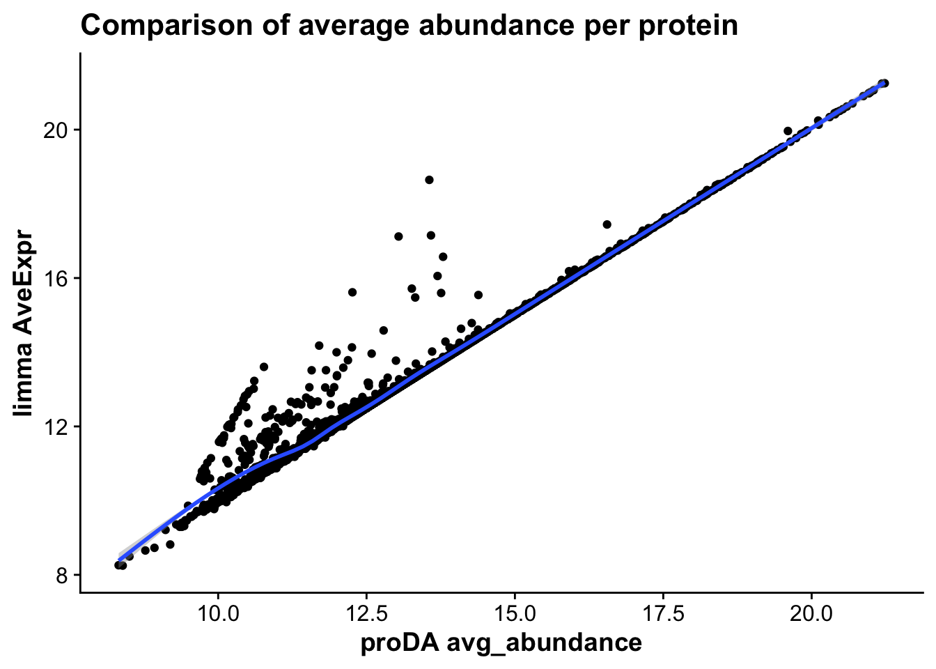
| Version | Author | Date |
|---|---|---|
| ed31d81 | FloWuenne | 2023-07-02 |
method_corr_mictr <- ggplot(merged_tests_mictr,aes(-log10(pval.x),-log10(P.Value),
                            label = gene)) +
  geom_point() +
  geom_smooth() +
  geom_vline(xintercept = -log10(0.05), linetype = 2) +
  geom_hline(yintercept = -log10(0.05), linetype = 2) +
  labs(x = "proDA -log10(pvalue)",
       y = "limma -log10(pvalue)",
       title = "Comparison of adjusted p-values")
method_corr_mictr
`geom_smooth()` using method = 'gam' and formula = 'y ~ s(x, bs = "cs")'Warning: Removed 114 rows containing non-finite values (`stat_smooth()`).Warning: The following aesthetics were dropped during statistical transformation: label
ℹ This can happen when ggplot fails to infer the correct grouping structure in
the data.
ℹ Did you forget to specify a `group` aesthetic or to convert a numerical
variable into a factor?Warning: Removed 114 rows containing missing values (`geom_point()`).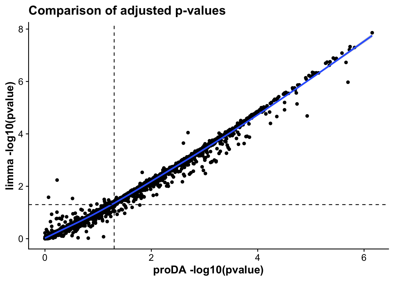
| Version | Author | Date |
|---|---|---|
| ed31d81 | FloWuenne | 2023-07-02 |
As we can see, the statistics across both proDA and limma correlate very strongly, suggesting that both methods provide similar results in terms of effect sizes and which genes are statistically significant.
The most significant difference between proDA and limma however, is that proDA can handle situations where all values are missing for one of the groups we want to compare. That means, that real proteins that are induced due to inflammation in MI_IZ samples but missing in controls during homeostasis of the tissue will have test statistics in proDA but not in limma results.
Let’s find these
## Which proteins could proDA test, that limma couldn't?
proda_only <- subset(merged_tests_mictr,is.na(adj.P.Val))
limma_only <- subset(merged_tests_mictr,is.na(adj_pval))
All of the proteins that could not be tested by limma contain fully or mostly missing values in the comparison made between control and MI.
sessionInfo()R version 4.2.3 (2023-03-15)
Platform: aarch64-apple-darwin20 (64-bit)
Running under: macOS Ventura 13.4.1
Matrix products: default
BLAS: /Library/Frameworks/R.framework/Versions/4.2-arm64/Resources/lib/libRblas.0.dylib
LAPACK: /Library/Frameworks/R.framework/Versions/4.2-arm64/Resources/lib/libRlapack.dylib
locale:
[1] en_US.UTF-8/en_US.UTF-8/en_US.UTF-8/C/en_US.UTF-8/en_US.UTF-8
attached base packages:
[1] stats graphics grDevices datasets utils methods base
other attached packages:
[1] vsn_3.66.0 Biobase_2.58.0 BiocGenerics_0.44.0
[4] plotly_4.10.2 eulerr_7.0.0 ggrepel_0.9.3
[7] pheatmap_1.0.12 limma_3.54.2 proDA_1.13.0
[10] here_1.0.1 cowplot_1.1.1 ggsci_3.0.0
[13] factoextra_1.0.7 lubridate_1.9.2 forcats_1.0.0
[16] stringr_1.5.0 dplyr_1.1.2 purrr_1.0.1
[19] readr_2.1.4 tidyr_1.3.0 tibble_3.2.1
[22] ggplot2_3.4.2 tidyverse_2.0.0 data.table_1.14.8
[25] workflowr_1.7.0
loaded via a namespace (and not attached):
[1] colorspace_2.1-0 ggsignif_0.6.4
[3] ellipsis_0.3.2 rprojroot_2.0.3
[5] XVector_0.38.0 GenomicRanges_1.50.2
[7] fs_1.6.2 rstudioapi_0.14
[9] ggpubr_0.6.0 farver_2.1.1
[11] hexbin_1.28.3 affyio_1.68.0
[13] fansi_1.0.4 splines_4.2.3
[15] cachem_1.0.8 knitr_1.42
[17] polyclip_1.10-4 jsonlite_1.8.4
[19] broom_1.0.5 BiocManager_1.30.21
[21] compiler_4.2.3 httr_1.4.6
[23] backports_1.4.1 Matrix_1.5-3
[25] fastmap_1.1.1 lazyeval_0.2.2
[27] cli_3.6.1 later_1.3.1
[29] htmltools_0.5.5 tools_4.2.3
[31] gtable_0.3.3 glue_1.6.2
[33] GenomeInfoDbData_1.2.9 affy_1.76.0
[35] Rcpp_1.0.10 carData_3.0-5
[37] jquerylib_0.1.4 vctrs_0.6.2
[39] nlme_3.1-162 preprocessCore_1.60.2
[41] crosstalk_1.2.0 polylabelr_0.2.0
[43] xfun_0.39 ps_1.7.4
[45] timechange_0.2.0 lifecycle_1.0.3
[47] renv_0.17.3 rstatix_0.7.2
[49] getPass_0.2-2 zlibbioc_1.44.0
[51] scales_1.2.1 hms_1.1.3
[53] promises_1.2.0.1 MatrixGenerics_1.10.0
[55] SummarizedExperiment_1.28.0 RColorBrewer_1.1-3
[57] yaml_2.3.7 sass_0.4.6
[59] stringi_1.7.12 highr_0.10
[61] S4Vectors_0.36.2 GenomeInfoDb_1.34.9
[63] rlang_1.1.1 pkgconfig_2.0.3
[65] matrixStats_1.0.0 bitops_1.0-7
[67] evaluate_0.21 lattice_0.20-45
[69] htmlwidgets_1.6.2 labeling_0.4.2
[71] processx_3.8.0 tidyselect_1.2.0
[73] magrittr_2.0.3 R6_2.5.1
[75] IRanges_2.32.0 generics_0.1.3
[77] DelayedArray_0.24.0 DBI_1.1.3
[79] mgcv_1.8-42 pillar_1.9.0
[81] whisker_0.4.1 withr_2.5.0
[83] abind_1.4-5 RCurl_1.98-1.12
[85] car_3.1-2 utf8_1.2.3
[87] tzdb_0.4.0 rmarkdown_2.21
[89] grid_4.2.3 callr_3.7.3
[91] git2r_0.32.0 digest_0.6.31
[93] extraDistr_1.9.1 httpuv_1.6.11
[95] stats4_4.2.3 munsell_0.5.0
[97] viridisLite_0.4.2 bslib_0.4.2