Applied Econometrics
Last updated: 2020-12-22
Checks: 6 1
Knit directory: R-Guide/
This reproducible R Markdown analysis was created with workflowr (version 1.6.2). The Checks tab describes the reproducibility checks that were applied when the results were created. The Past versions tab lists the development history.
The R Markdown file has unstaged changes. To know which version of the R Markdown file created these results, you’ll want to first commit it to the Git repo. If you’re still working on the analysis, you can ignore this warning. When you’re finished, you can run wflow_publish to commit the R Markdown file and build the HTML.
Great job! The global environment was empty. Objects defined in the global environment can affect the analysis in your R Markdown file in unknown ways. For reproduciblity it’s best to always run the code in an empty environment.
The command set.seed(20201221) was run prior to running the code in the R Markdown file. Setting a seed ensures that any results that rely on randomness, e.g. subsampling or permutations, are reproducible.
Great job! Recording the operating system, R version, and package versions is critical for reproducibility.
Nice! There were no cached chunks for this analysis, so you can be confident that you successfully produced the results during this run.
Great job! Using relative paths to the files within your workflowr project makes it easier to run your code on other machines.
Great! You are using Git for version control. Tracking code development and connecting the code version to the results is critical for reproducibility.
The results in this page were generated with repository version 7a501fa. See the Past versions tab to see a history of the changes made to the R Markdown and HTML files.
Note that you need to be careful to ensure that all relevant files for the analysis have been committed to Git prior to generating the results (you can use wflow_publish or wflow_git_commit). workflowr only checks the R Markdown file, but you know if there are other scripts or data files that it depends on. Below is the status of the Git repository when the results were generated:
Ignored files:
    Ignored:    .RData
    Ignored:    .Rhistory
    Ignored:    .Rproj.user/

Untracked files:
    Untracked:  data/cancer_test.xlsx

Unstaged changes:
    Modified:   analysis/index.Rmd
Note that any generated files, e.g. HTML, png, CSS, etc., are not included in this status report because it is ok for generated content to have uncommitted changes.
These are the previous versions of the repository in which changes were made to the R Markdown (analysis/index.Rmd) and HTML (docs/index.html) files. If you’ve configured a remote Git repository (see ?wflow_git_remote), click on the hyperlinks in the table below to view the files as they were in that past version.
| File | Version | Author | Date | Message |
|---|---|---|---|---|
| Rmd | 7a501fa | KaranSShakya | 2020-12-22 | TOC re-edited + correlation one var. |
| html | 7a501fa | KaranSShakya | 2020-12-22 | TOC re-edited + correlation one var. |
| Rmd | a494ed3 | KaranSShakya | 2020-12-21 | TOC FINAL FIX |
| html | a494ed3 | KaranSShakya | 2020-12-21 | TOC FINAL FIX |
| Rmd | 2eaade1 | KaranSShakya | 2020-12-21 | toc test againa |
| html | 2eaade1 | KaranSShakya | 2020-12-21 | toc test againa |
| Rmd | 3a2205e | KaranSShakya | 2020-12-21 | toc fix attempt? |
| html | 3a2205e | KaranSShakya | 2020-12-21 | toc fix attempt? |
| Rmd | 261ae64 | KaranSShakya | 2020-12-21 | toc fix with new format |
| html | 261ae64 | KaranSShakya | 2020-12-21 | toc fix with new format |
| Rmd | 81c56de | KaranSShakya | 2020-12-21 | toc changes final maybe |
| html | 81c56de | KaranSShakya | 2020-12-21 | toc changes final maybe |
| Rmd | b501120 | KaranSShakya | 2020-12-21 | toc collapse change |
| html | b501120 | KaranSShakya | 2020-12-21 | toc collapse change |
| Rmd | c9f84cd | KaranSShakya | 2020-12-21 | toc fix html |
| html | c9f84cd | KaranSShakya | 2020-12-21 | toc fix html |
| Rmd | df6b3c2 | KaranSShakya | 2020-12-21 | toc fixing test |
| html | df6b3c2 | KaranSShakya | 2020-12-21 | toc fixing test |
| Rmd | 7499ecb | KaranSShakya | 2020-12-21 | toc fix depth 2 |
| html | 7499ecb | KaranSShakya | 2020-12-21 | toc fix depth 2 |
| Rmd | 859395e | KaranSShakya | 2020-12-21 | toc fix |
| html | 859395e | KaranSShakya | 2020-12-21 | toc fix |
| Rmd | 63011cb | KaranSShakya | 2020-12-21 | First commits |
| html | 63011cb | KaranSShakya | 2020-12-21 | First commits |
| Rmd | c9dd7d1 | KaranSShakya | 2020-12-21 | Start workflowr project. |
1 Setting Up
1.1 Packages
tidyverse - basic package for data wrangling
readxl - allows inputs of excel files
readr - allows inputs of text files
broom - result organization with tidy tibbles
stargazer - better organized regression outputs
1.2 Output Tables
2 Initial Statistics
2.1 Correlation
2.1.1 One Variable
Correlation is the strength of linear assosciation. It can be sensitive to outliers.
cor <- corr_1 %>%
  summarise(r=cor(X, Y)) %>%
  pull(r)
cor
[1] 0.8351438Correlations can also be visualized through scatterplots which are the foundation of econometric analysis.
ggplot(corr_1, aes(x=X, y=Y))+
  geom_point(alpha=0.5)+
  geom_smooth(method = "lm", se=F)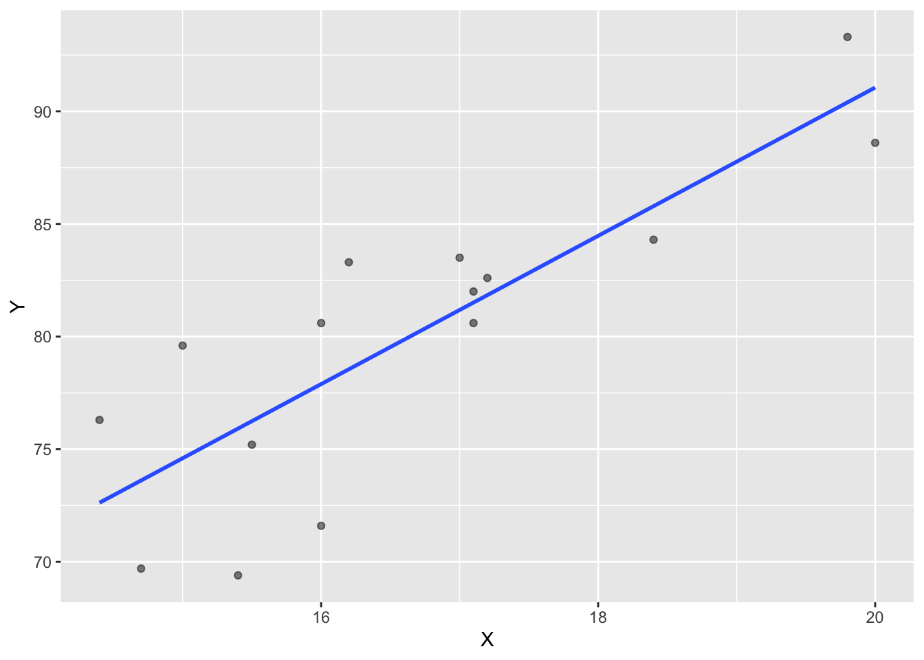
| Version | Author | Date |
|---|---|---|
| 7a501fa | KaranSShakya | 2020-12-22 |
2.1.2 Multiple Variables
3 Simple Linear Regression
Linear regression can be performed by:
lm.model <- lm(Cancer_Diagnosis~Median_Income+Median_Age+Percent_Black, data=cancer_test)
lm.res <- augment(lm.model) # visualize all residuals in table form
3.1 Least Square Lines
The following code is for two variables:
lm.ls <- lm.res %>%
  summarize(x.sd=sd(Median_Age), y.sd=sd(Cancer_Diagnosis),
            cor=cor(Cancer_Diagnosis, Median_Age)) %>%
  mutate(slope=(x.sd/y.sd)*cor) # Slope = 0.015
When we look at the lm model, the slope is also 0.015.
3.2 Visualizing Assumptions
a. Linearity (scatterplot + residual plot - residuals needs to be random)
b. Nearly normal residuals (histogram of residuals or QQ residual plot)
c. Constant variability (residual plot)
Link for interactive regression diagnostic test.
a <- ggplot(lm.res, aes(x=.fitted, y=.resid))+
  geom_point()+
  geom_hline(yintercept = 0, linetype="dashed", color="red")+
  labs(title="Residuals vs Fitted Values", x="Fitted Values", y="Residuals")
b <- ggplot(lm.res, aes(x=.resid))+
  geom_density()+
  labs(title="Histogram of residuals", x="Residuals") #geom_density can also be added
c <- ggplot(lm.res, aes(sample=.resid))+
  stat_qq()+
  stat_qq_line()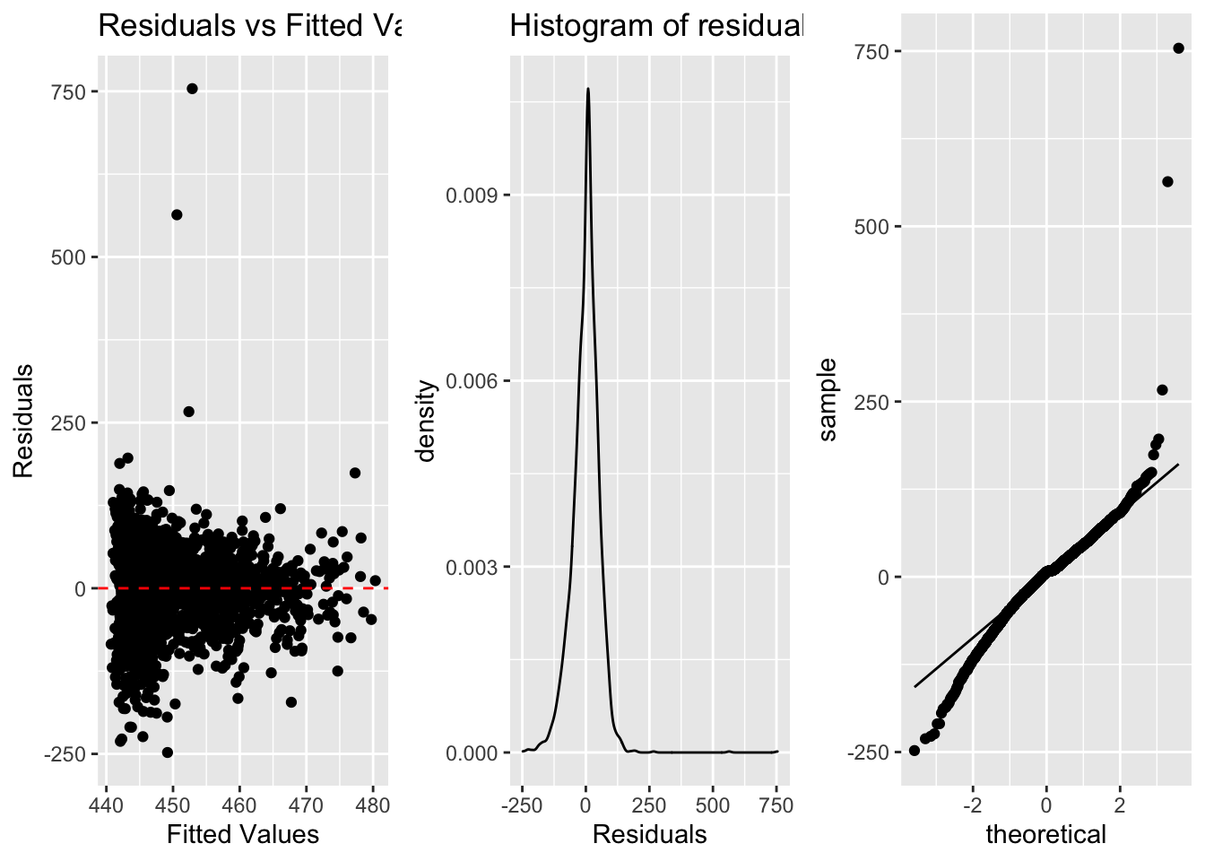
3.3 Dummy Variables
4 Hypothesis Testing
sessionInfo()R version 4.0.0 (2020-04-24)
Platform: x86_64-apple-darwin17.0 (64-bit)
Running under: macOS 10.16
Matrix products: default
BLAS: /Library/Frameworks/R.framework/Versions/4.0/Resources/lib/libRblas.dylib
LAPACK: /Library/Frameworks/R.framework/Versions/4.0/Resources/lib/libRlapack.dylib
locale:
[1] en_US.UTF-8/en_US.UTF-8/en_US.UTF-8/C/en_US.UTF-8/en_US.UTF-8
attached base packages:
[1] stats graphics grDevices utils datasets methods base
other attached packages:
[1] gridExtra_2.3 broom_0.5.6 readxl_1.3.1 forcats_0.5.0
[5] stringr_1.4.0 dplyr_0.8.5 purrr_0.3.4 readr_1.3.1
[9] tidyr_1.0.3 tibble_3.0.1 ggplot2_3.3.0 tidyverse_1.3.0
[13] workflowr_1.6.2
loaded via a namespace (and not attached):
[1] Rcpp_1.0.4.6 lubridate_1.7.8 lattice_0.20-41 assertthat_0.2.1
[5] rprojroot_1.3-2 digest_0.6.25 R6_2.4.1 cellranger_1.1.0
[9] backports_1.1.6 reprex_0.3.0 evaluate_0.14 httr_1.4.1
[13] pillar_1.4.4 rlang_0.4.6 rstudioapi_0.11 whisker_0.4
[17] Matrix_1.2-18 rmarkdown_2.6 labeling_0.3 splines_4.0.0
[21] munsell_0.5.0 compiler_4.0.0 httpuv_1.5.2 modelr_0.1.7
[25] xfun_0.19 pkgconfig_2.0.3 mgcv_1.8-31 htmltools_0.5.0
[29] tidyselect_1.1.0 fansi_0.4.1 crayon_1.3.4 dbplyr_1.4.3
[33] withr_2.2.0 later_1.0.0 grid_4.0.0 nlme_3.1-147
[37] jsonlite_1.6.1 gtable_0.3.0 lifecycle_0.2.0 DBI_1.1.0
[41] git2r_0.27.1 magrittr_1.5 scales_1.1.1 cli_2.0.2
[45] stringi_1.4.6 farver_2.0.3 fs_1.4.1 promises_1.1.0
[49] xml2_1.3.2 ellipsis_0.3.0 generics_0.0.2 vctrs_0.3.0
[53] tools_4.0.0 glue_1.4.1 hms_0.5.3 yaml_2.2.1
[57] colorspace_1.4-1 rvest_0.3.5 knitr_1.28 haven_2.2.0