Applied Econometrics
Last updated: 2020-12-27
Checks: 6 1
Knit directory: R-Guide/
This reproducible R Markdown analysis was created with workflowr (version 1.6.2). The Checks tab describes the reproducibility checks that were applied when the results were created. The Past versions tab lists the development history.
The R Markdown file has unstaged changes. To know which version of the R Markdown file created these results, you’ll want to first commit it to the Git repo. If you’re still working on the analysis, you can ignore this warning. When you’re finished, you can run wflow_publish to commit the R Markdown file and build the HTML.
Great job! The global environment was empty. Objects defined in the global environment can affect the analysis in your R Markdown file in unknown ways. For reproduciblity it’s best to always run the code in an empty environment.
The command set.seed(20201221) was run prior to running the code in the R Markdown file. Setting a seed ensures that any results that rely on randomness, e.g. subsampling or permutations, are reproducible.
Great job! Recording the operating system, R version, and package versions is critical for reproducibility.
Nice! There were no cached chunks for this analysis, so you can be confident that you successfully produced the results during this run.
Great job! Using relative paths to the files within your workflowr project makes it easier to run your code on other machines.
Great! You are using Git for version control. Tracking code development and connecting the code version to the results is critical for reproducibility.
The results in this page were generated with repository version b07f4c3. See the Past versions tab to see a history of the changes made to the R Markdown and HTML files.
Note that you need to be careful to ensure that all relevant files for the analysis have been committed to Git prior to generating the results (you can use wflow_publish or wflow_git_commit). workflowr only checks the R Markdown file, but you know if there are other scripts or data files that it depends on. Below is the status of the Git repository when the results were generated:
Ignored files:
    Ignored:    .RData
    Ignored:    .Rhistory
    Ignored:    .Rproj.user/

Unstaged changes:
    Modified:   analysis/econometrics.Rmd
    Modified:   analysis/q_8731_hw3.Rmd
Note that any generated files, e.g. HTML, png, CSS, etc., are not included in this status report because it is ok for generated content to have uncommitted changes.
These are the previous versions of the repository in which changes were made to the R Markdown (analysis/econometrics.Rmd) and HTML (docs/econometrics.html) files. If you’ve configured a remote Git repository (see ?wflow_git_remote), click on the hyperlinks in the table below to view the files as they were in that past version.
| File | Version | Author | Date | Message |
|---|---|---|---|---|
| Rmd | b07f4c3 | KaranSShakya | 2020-12-27 | econometrics problems page + data |
| html | b07f4c3 | KaranSShakya | 2020-12-27 | econometrics problems page + data |
| Rmd | 5759bf7 | KaranSShakya | 2020-12-26 | organizational fixes |
| html | 5759bf7 | KaranSShakya | 2020-12-26 | organizational fixes |
| Rmd | 1242c7c | KaranSShakya | 2020-12-26 | Data distribution |
| html | 1242c7c | KaranSShakya | 2020-12-26 | Data distribution |
| Rmd | 07e9daf | KaranSShakya | 2020-12-25 | manual LS examples |
| html | 07e9daf | KaranSShakya | 2020-12-25 | manual LS examples |
| html | e2b1935 | KaranSShakya | 2020-12-24 | site_yml ordering correction |
| Rmd | 924d00b | KaranSShakya | 2020-12-24 | Overall formatting + new sections |
| html | 924d00b | KaranSShakya | 2020-12-24 | Overall formatting + new sections |
1 Setting Up
1.1 Packages
tidyverse - basic package for data wrangling
readxl - allows inputs of excel files
readr - allows inputs of text files
jtools -
summfunctions for better regression outputsbroom - result organization with tidy tibbles
stargazer - better organized regression outputs
sandwitch - robust standard errors
1.2 Output Tables
Here is a basic example of linear regression. Age and Weight of an individual is used to predict the blood pressure.
model <- lm(bloodp~age+weight, data=bloodp)
summ(model)
MODEL INFO:
Observations: 11
Dependent Variable: bloodp
Type: OLS linear regression
MODEL FIT:
F(2,8) = 168.76, p = 0.00
R² = 0.98
Adj. R² = 0.97
Standard errors: OLS
-------------------------------------------------
Est. S.E. t val. p
----------------- ------- ------- -------- ------
(Intercept) 30.99 11.94 2.59 0.03
age 0.86 0.25 3.47 0.01
weight 0.33 0.13 2.56 0.03
-------------------------------------------------The function summ is good and direct in printing output. The base r summary is okay to use, and the more intricate stargazer is good too.
summ will be used mostly here when printing regression outputs.
2 Correlation
2.1 One Variable
Correlation is the strength of linear assosciation. It can be sensitive to outliers. The pull function is used to print out the correlation value more.
cor <- corr_1 %>%
  summarise(r=cor(X, Y)) %>%
  pull(r)
cor
[1] 0.8351438Observing correlation from regression. Sqrt of R^2 is correlation.
cor.lm <- lm(Y~X, data=corr_1)
summ(cor.lm)
MODEL INFO:
Observations: 15
Dependent Variable: Y
Type: OLS linear regression
MODEL FIT:
F(1,13) = 29.97, p = 0.00
R² = 0.70
Adj. R² = 0.67
Standard errors: OLS
-------------------------------------------------
Est. S.E. t val. p
----------------- ------- ------- -------- ------
(Intercept) 25.23 10.06 2.51 0.03
X 3.29 0.60 5.47 0.00
-------------------------------------------------Or using base r function cor:
cor.2 <- cor(corr_1)
cor.2
X Y
X 1.0000000 0.8351438
Y 0.8351438 1.0000000Correlations can also be visualized through scatterplots which important to any econometric analysis. Method = “lm” produces the blue linear regression line.
ggplot(corr_1, aes(x=X, y=Y))+
  geom_point(alpha=0.5)+
  geom_smooth(method = "lm", se=F)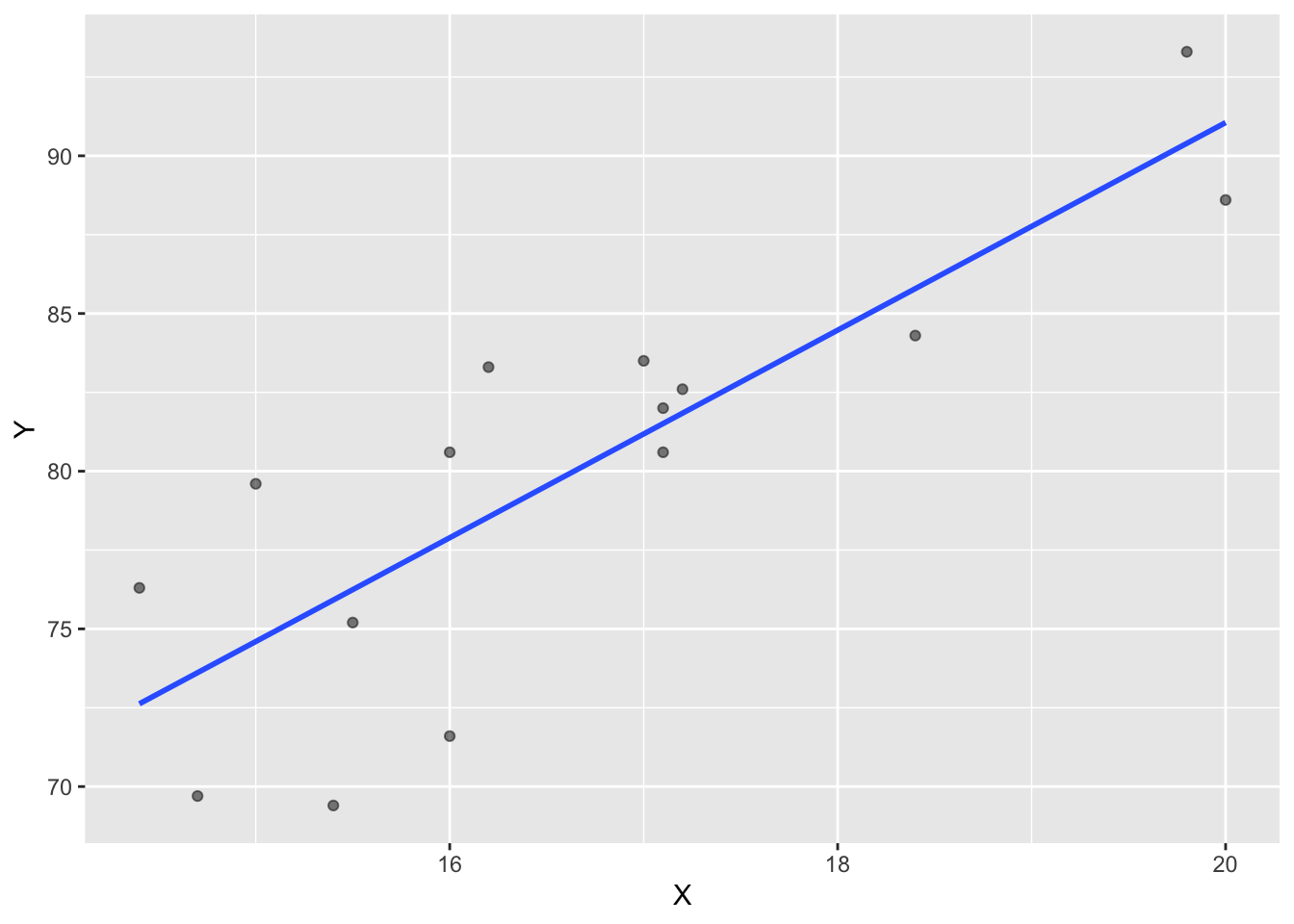
Or, you can use the effects plot. This is an example of the blood pressure model.
effect_plot(model, pred = age, interval = T, plot.points = T)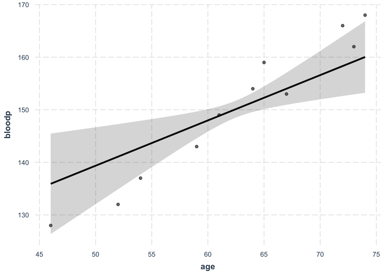
| Version | Author | Date |
|---|---|---|
| 5759bf7 | KaranSShakya | 2020-12-26 |
2.2 Multiple Variables
Multiple variables can be tabulated against eachother to observe the correlation. In this example, cancer diagnosis ~ income + age + private + public + per_white + per_black
Viewing correlation table:
cor.cancer <- cor(cancer.2)
cor.cancer
Cancer_Diagnosis Median_Income Median_Age Private_Coverage
Cancer_Diagnosis 1.000000000 -0.001036186 0.018089172 0.105174269
Median_Income -0.001036186 1.000000000 -0.013287743 0.724174768
Median_Age 0.018089172 -0.013287743 1.000000000 0.004665111
Private_Coverage 0.105174269 0.724174768 0.004665111 1.000000000
Public_Coverage 0.046108610 -0.754821751 0.049060211 -0.720011521
Percent_White -0.014509829 0.167225441 0.035009366 0.429031447
Percent_Black 0.113488959 -0.270231619 -0.017173240 -0.345172126
Public_Coverage Percent_White Percent_Black
Cancer_Diagnosis 0.04610861 -0.01450983 0.11348896
Median_Income -0.75482175 0.16722544 -0.27023162
Median_Age 0.04906021 0.03500937 -0.01717324
Private_Coverage -0.72001152 0.42903145 -0.34517213
Public_Coverage 1.00000000 -0.13370507 0.19559747
Percent_White -0.13370507 1.00000000 -0.82845885
Percent_Black 0.19559747 -0.82845885 1.00000000Viewing in diagrams:
ggpairs(cancer.2)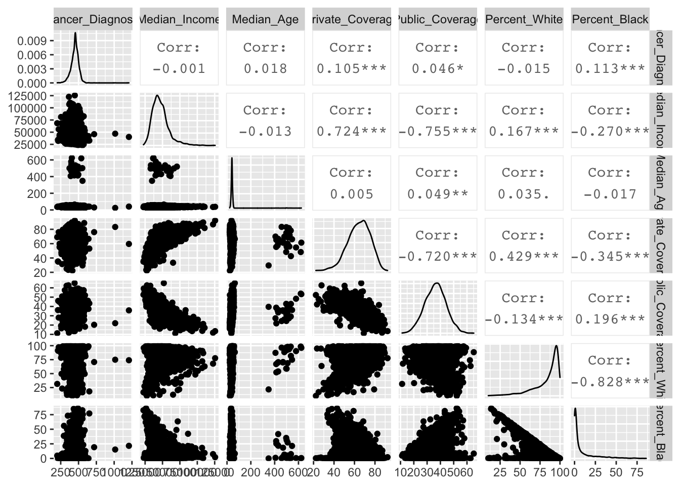
| Version | Author | Date |
|---|---|---|
| 5759bf7 | KaranSShakya | 2020-12-26 |
3 Understanding Linear Regression
cancer diagnosis ~ income + age + private + public + per_white + per_black model is used in the following examples.
lm.model <- lm(Cancer_Diagnosis~Median_Income+Median_Age+Private_Coverage+Public_Coverage+Percent_White+Percent_Black, data=cancer.2)
summ(lm.model)
MODEL INFO:
Observations: 3047
Dependent Variable: Cancer_Diagnosis
Type: OLS linear regression
MODEL FIT:
F(6,3040) = 40.40, p = 0.00
R² = 0.07
Adj. R² = 0.07
Standard errors: OLS
-------------------------------------------------------
Est. S.E. t val. p
---------------------- -------- ------- -------- ------
(Intercept) 245.57 16.73 14.68 0.00
Median_Income -0.00 0.00 -0.25 0.80
Median_Age 0.01 0.02 0.33 0.74
Private_Coverage 1.75 0.17 10.36 0.00
Public_Coverage 1.73 0.21 8.40 0.00
Percent_White 0.24 0.12 2.01 0.04
Percent_Black 0.91 0.13 7.16 0.00
-------------------------------------------------------To visualize the residual table we use the function augment.
lm.res <- augment(lm.model) 3.1 Least Square Lines
The least square estimator is: \[ \sum_{i=1}^{n} (Y_i-\beta_0-\beta_1 X_i)^2 \] The estimators can be calculated as follows: \[ \begin{align} \beta_1 &= \frac{\sum_{i=1}^n (X_i - \bar{X})(Y_i-\bar{Y})}{\sum_{i=1}^{n}(X_1-\bar{X})^2}\\ \\ \beta_0 &= \bar{Y} - \hat{\beta_1} \bar{X} \end{align} \]
We can manually do these calculations. To do these we use the package AER and load the CASchool dataset.
Lets conduct a simple linear regression score ~ STR (STR = student teacher ratio).
ca.model <- lm(Score~Str, data=ca.data)
summ(ca.model)
MODEL INFO:
Observations: 420
Dependent Variable: Score
Type: OLS linear regression
MODEL FIT:
F(1,418) = 22.58, p = 0.00
R² = 0.05
Adj. R² = 0.05
Standard errors: OLS
-------------------------------------------------
Est. S.E. t val. p
----------------- -------- ------ -------- ------
(Intercept) 698.93 9.47 73.82 0.00
Str -2.28 0.48 -4.75 0.00
-------------------------------------------------Manually computing the estimators.
attach(ca.data)
beta_1 <- sum((Str-mean(Str))*(Score-mean(Score))) / sum((Str-mean(Str))^2)
beta_1
[1] -2.279808beta_0 <- mean(Score) - beta_1*mean(Str)
beta_0[1] 698.93293.2 Goodness of Fit
We need to understand: Explained Sum of Squares (ESS), Total Sum of Squares (TSS), and Sum of Square Residuals (SSR). $$ \[\begin{align} ESS &= \sum_{i=1}^{n} (\hat{Y_i}-\bar{Y})^2\\ TSS &= \sum_{i=1}^{n} (Y_i - \bar{Y})^2\\ R^2 &= \frac{ESS}{TSS} \\ \\ SSR &= \sum_{i=1}^{n} \hat{u_i}^2\\ TSS &= ESS + SSR\\ R^2 &= 1-\frac{SSR}{TSS} \end{align}\] $$ We can calculate the Standard Error of Regression (SER) as \(s^2=\frac{SSR}{n-2}\)
Computing these goodness of fit values manually.
ca.summary <- summary(ca.model)
SSR <- sum(ca.summary$residuals^2)
TSS <- sum((Score-mean(Score))^2)
R_sq <- 1 - SSR/TSS
R_sq
[1] 0.05124009detach(ca.data)3.3 Least Square Assumptions
a. Linearity (scatterplot + residual plot - residuals needs to be random)
b. Nearly normal residuals (histogram of residuals or QQ residual plot)
c. Constant variability (residual plot)
Link for interactive regression diagnostic test.
a <- ggplot(lm.res, aes(x=.fitted, y=.resid))+
  geom_point()+
  geom_hline(yintercept = 0, linetype="dashed", color="red")+
  labs(title="Residuals vs Fitted Values", x="Fitted Values", y="Residuals")
b <- ggplot(lm.res, aes(x=.resid))+
  geom_density()+
  labs(title="Histogram of residuals", x="Residuals") #geom_density can also be added
c <- ggplot(lm.res, aes(sample=.resid))+
  stat_qq()+
  stat_qq_line()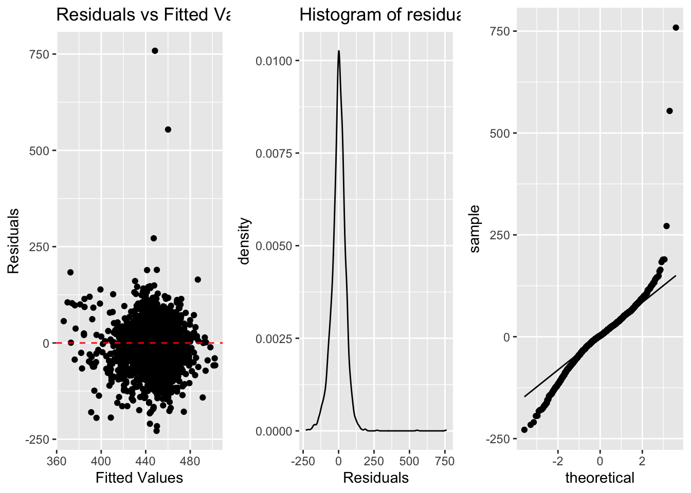
| Version | Author | Date |
|---|---|---|
| 5759bf7 | KaranSShakya | 2020-12-26 |
3.4 Covariance Matrix
Covaraince matrix can be created using vocv.
vcov(lm.model) (Intercept) Median_Income Median_Age Private_Coverage
(Intercept) 279.895460469 -1.117642e-03 3.524437e-03 -9.377888e-01
Median_Income -0.001117642 1.921940e-08 -5.465260e-08 -1.062539e-05
Median_Age 0.003524437 -5.465260e-08 4.446881e-04 -9.975174e-05
Private_Coverage -0.937788802 -1.062539e-05 -9.975174e-05 2.851442e-02
Public_Coverage -2.612435764 1.144682e-05 -2.902941e-04 1.503650e-02
Percent_White -0.751040921 5.216770e-06 -4.661584e-05 -1.049701e-02
Percent_Black -0.951741623 5.275435e-06 -2.654088e-05 -6.561322e-03
Public_Coverage Percent_White Percent_Black
(Intercept) -2.612436e+00 -7.510409e-01 -9.517416e-01
Median_Income 1.144682e-05 5.216770e-06 5.275435e-06
Median_Age -2.902941e-04 -4.661584e-05 -2.654088e-05
Private_Coverage 1.503650e-02 -1.049701e-02 -6.561322e-03
Public_Coverage 4.239607e-02 -4.719157e-03 -2.531219e-03
Percent_White -4.719157e-03 1.479425e-02 1.282179e-02
Percent_Black -2.531219e-03 1.282179e-02 1.605172e-024 Robust Standard Errors
This requires the sandwitch package. There are many robust standard error (heteroskedasctic errors) parameters ranging from HC0 to HC5. The default for STATA is HC1 which is important to keep in mind if we are trying to emulate STATA result.
model <- lm(bloodp~age+weight, data=bloodp)
summ(model, robust = "HC1")
MODEL INFO:
Observations: 11
Dependent Variable: bloodp
Type: OLS linear regression
MODEL FIT:
F(2,8) = 168.76, p = 0.00
R² = 0.98
Adj. R² = 0.97
Standard errors: Robust, type = HC1
-------------------------------------------------
Est. S.E. t val. p
----------------- ------- ------- -------- ------
(Intercept) 30.99 10.60 2.92 0.02
age 0.86 0.30 2.92 0.02
weight 0.33 0.14 2.33 0.05
-------------------------------------------------5 Dummy Variables
Group 1, Group 2, and Group 3 are all dummy variables (0 or 1). When regressors are dummy variables you need to regress it without the intercept term.
reg <- lm(Earnings ~ -1+Group1+Group2+Group3, data=dummy)
summ(reg)
MODEL INFO:
Observations: 4266
Dependent Variable: Earnings
Type: OLS linear regression
MODEL FIT:
F(3,4263) = 3842.49, p = 0.00
R² = 0.73
Adj. R² = 0.73
Standard errors: OLS
------------------------------------------------
Est. S.E. t val. p
------------ ---------- -------- -------- ------
Group1 22880.48 467.45 48.95 0.00
Group2 25080.17 380.02 66.00 0.00
Group3 27973.63 404.78 69.11 0.00
------------------------------------------------If we want to add the intercept term, one of the dummy variables needs to be removed to avoid collinearity with the intercept term.
reg2 <- lm(Earnings~Group1+Group2, data=dummy)
summ(reg2)MODEL INFO:
Observations: 4266
Dependent Variable: Earnings
Type: OLS linear regression
MODEL FIT:
F(2,4263) = 34.98, p = 0.00
R² = 0.02
Adj. R² = 0.02
Standard errors: OLS
-----------------------------------------------------
Est. S.E. t val. p
----------------- ---------- -------- -------- ------
(Intercept) 27973.63 404.78 69.11 0.00
Group1 -5093.16 618.35 -8.24 0.00
Group2 -2893.46 555.21 -5.21 0.00
-----------------------------------------------------6 Lagged Regression
lag1 <- lag %>%
mutate(Work_1 = lag(Work, 1)) %>%
mutate(Work_2 = lag(Work, 2))
kable(head(lag1))| Year | Income | Work | Work_1 | Work_2 |
|---|---|---|---|---|
| 2000 | 55 | 30 | NA | NA |
| 2001 | 60 | 31 | 30 | NA |
| 2002 | 65 | 32 | 31 | 30 |
| 2003 | 70 | 33 | 32 | 31 |
| 2004 | 75 | 34 | 33 | 32 |
| 2005 | 80 | 35 | 34 | 33 |
Using this we can perform linear regression the normal way:
reg.lag <- lm(Income ~ Work+Work_1+Work_2, data=dataset)Warning in remove(reg.lag, lag, lag1): object 'reg.lag' not found7 Hypothesis Testing
7.1 Confidence Interval
There are two methods that can be used. The base r confint and summ. Both examples are below. The dummy variable regression result is used as example.
MODEL INFO:
Observations: 4266
Dependent Variable: Earnings
Type: OLS linear regression

MODEL FIT:
F(3,4263) = 3842.49, p = 0.00
R² = 0.73
Adj. R² = 0.73

Standard errors: OLS
------------------------------------------------
                   Est.     S.E.   t val.      p
------------ ---------- -------- -------- ------
Group1         22880.48   467.45    48.95   0.00
Group2         25080.17   380.02    66.00   0.00
Group3         27973.63   404.78    69.11   0.00
------------------------------------------------The confint method to find a 95% CI is,
confint(reg, level=0.95) 2.5 % 97.5 %
Group1 21964.03 23796.92
Group2 24335.14 25825.21
Group3 27180.06 28767.21The summ method to find a 95% CI is,
summ(reg, confint = TRUE, ci.width = 0.95, digits = 3)MODEL INFO:
Observations: 4266
Dependent Variable: Earnings
Type: OLS linear regression
MODEL FIT:
F(3,4263) = 3842.486, p = 0.000
R² = 0.730
Adj. R² = 0.730
Standard errors: OLS
-----------------------------------------------------------------
Est. 2.5% 97.5% t val. p
------------ ----------- ----------- ----------- -------- -------
Group1 22880.476 21964.029 23796.922 48.947 0.000
Group2 25080.174 24335.139 25825.209 65.997 0.000
Group3 27973.635 27180.058 28767.211 69.109 0.000
-----------------------------------------------------------------7.2 t-test b=0
For this we will be using the score~STR regression.
summ(ca.model)MODEL INFO:
Observations: 420
Dependent Variable: Score
Type: OLS linear regression
MODEL FIT:
F(1,418) = 22.58, p = 0.00
R² = 0.05
Adj. R² = 0.05
Standard errors: OLS
-------------------------------------------------
Est. S.E. t val. p
----------------- -------- ------ -------- ------
(Intercept) 698.93 9.47 73.82 0.00
Str -2.28 0.48 -4.75 0.00
-------------------------------------------------\[ \begin{align} H_0: \beta_1 = 0 &&& H_1: \beta_1 \neq 0 \end{align} \]
Testing this hypothesis manually: \[
t = \frac{-2.2798 - 0}{0.4798} = -4.75
\] This means we reject the null hypothesis at 5% because the level of significance is \(|t| > 1.96\). This is what the summ results in t val and p.
7.3 Joint Hypothesis
\[ F = \frac{(SSR_{restricted} - SSR_{unrestricted})/q}{SSR_{unrestricted}/(n-k-1)} \]
MODEL INFO:
Observations: 420
Dependent Variable: Score
Type: OLS linear regression

MODEL FIT:
F(3,416) = 107.455, p = 0.000
R² = 0.437
Adj. R² = 0.433

Standard errors: OLS
------------------------------------------------------
                       Est.     S.E.    t val.       p
----------------- --------- -------- --------- -------
(Intercept)         649.578   15.206    42.719   0.000
expenditure           0.004    0.001     2.739   0.006
Str                  -0.286    0.481    -0.596   0.551
english              -0.656    0.039   -16.776   0.000
------------------------------------------------------
Testing the joint hypothesis that Str = 0 and english = 0. We use the function linearHypothesis.
linearHypothesis(model.f, c("Str=0", "english=0"))Linear hypothesis test
Hypothesis:
Str = 0
english = 0
Model 1: restricted model
Model 2: Score ~ expenditure + Str + english
Res.Df RSS Df Sum of Sq F Pr(>F)
1 418 146545
2 416 85700 2 60845 147.68 < 2.2e-16 ***
---
Signif. codes: 0 '***' 0.001 '**' 0.01 '*' 0.05 '.' 0.1 ' ' 1F - stat is 147.68 and P-value is 2.2e-16 thus reject that null hypothesis.
A heteroskedastic-robust F test can also be conducted by adding white.adjust.
linearHypothesis(model.f, c("Str=0", "english=0"), white.adjust = "hc1")Linear hypothesis test
Hypothesis:
Str = 0
english = 0
Model 1: restricted model
Model 2: Score ~ expenditure + Str + english
Note: Coefficient covariance matrix supplied.
Res.Df Df F Pr(>F)
1 418
2 416 2 220.77 < 2.2e-16 ***
---
Signif. codes: 0 '***' 0.001 '**' 0.01 '*' 0.05 '.' 0.1 ' ' 18 Testing Multiple Models
sessionInfo()R version 4.0.0 (2020-04-24)
Platform: x86_64-apple-darwin17.0 (64-bit)
Running under: macOS 10.16
Matrix products: default
BLAS: /Library/Frameworks/R.framework/Versions/4.0/Resources/lib/libRblas.dylib
LAPACK: /Library/Frameworks/R.framework/Versions/4.0/Resources/lib/libRlapack.dylib
locale:
[1] en_US.UTF-8/en_US.UTF-8/en_US.UTF-8/C/en_US.UTF-8/en_US.UTF-8
attached base packages:
[1] stats graphics grDevices utils datasets methods base
other attached packages:
[1] AER_1.2-9 survival_3.1-12 sandwich_3.0-0 lmtest_0.9-38
[5] zoo_1.8-8 car_3.0-10 carData_3.0-4 gridExtra_2.3
[9] GGally_2.0.0 jtools_2.1.1 stargazer_5.2.2 broom_0.5.6
[13] readxl_1.3.1 forcats_0.5.0 stringr_1.4.0 dplyr_0.8.5
[17] purrr_0.3.4 readr_1.3.1 tidyr_1.0.3 tibble_3.0.1
[21] ggplot2_3.3.0 tidyverse_1.3.0 knitr_1.28 workflowr_1.6.2
loaded via a namespace (and not attached):
[1] nlme_3.1-147 fs_1.4.1 lubridate_1.7.8 RColorBrewer_1.1-2
[5] httr_1.4.1 rprojroot_1.3-2 tools_4.0.0 backports_1.1.6
[9] R6_2.4.1 DBI_1.1.0 mgcv_1.8-31 colorspace_1.4-1
[13] withr_2.2.0 tidyselect_1.1.0 curl_4.3 compiler_4.0.0
[17] git2r_0.27.1 cli_2.0.2 rvest_0.3.5 xml2_1.3.2
[21] labeling_0.3 scales_1.1.1 digest_0.6.25 foreign_0.8-78
[25] rmarkdown_2.6 rio_0.5.16 pkgconfig_2.0.3 htmltools_0.5.0
[29] highr_0.8 dbplyr_1.4.3 rlang_0.4.6 rstudioapi_0.11
[33] farver_2.0.3 generics_0.0.2 jsonlite_1.6.1 zip_2.0.4
[37] magrittr_1.5 Formula_1.2-3 Matrix_1.2-18 Rcpp_1.0.4.6
[41] munsell_0.5.0 fansi_0.4.1 abind_1.4-5 lifecycle_0.2.0
[45] stringi_1.4.6 whisker_0.4 yaml_2.2.1 plyr_1.8.6
[49] grid_4.0.0 promises_1.1.0 crayon_1.3.4 lattice_0.20-41
[53] haven_2.2.0 splines_4.0.0 pander_0.6.3 hms_0.5.3
[57] pillar_1.4.4 reprex_0.3.0 glue_1.4.1 evaluate_0.14
[61] data.table_1.12.8 modelr_0.1.7 vctrs_0.3.0 httpuv_1.5.2
[65] cellranger_1.1.0 gtable_0.3.0 reshape_0.8.8 assertthat_0.2.1
[69] xfun_0.19 openxlsx_4.1.5 later_1.0.0 ellipsis_0.3.0