Base R Statistics
Last updated: 2020-05-20
Checks: 7 0
Knit directory: R-codes/
This reproducible R Markdown analysis was created with workflowr (version 1.6.2). The Checks tab describes the reproducibility checks that were applied when the results were created. The Past versions tab lists the development history.
Great! Since the R Markdown file has been committed to the Git repository, you know the exact version of the code that produced these results.
Great job! The global environment was empty. Objects defined in the global environment can affect the analysis in your R Markdown file in unknown ways. For reproduciblity it’s best to always run the code in an empty environment.
The command set.seed(20200515) was run prior to running the code in the R Markdown file. Setting a seed ensures that any results that rely on randomness, e.g. subsampling or permutations, are reproducible.
Great job! Recording the operating system, R version, and package versions is critical for reproducibility.
Nice! There were no cached chunks for this analysis, so you can be confident that you successfully produced the results during this run.
Great job! Using relative paths to the files within your workflowr project makes it easier to run your code on other machines.
Great! You are using Git for version control. Tracking code development and connecting the code version to the results is critical for reproducibility.
The results in this page were generated with repository version 2da8824. See the Past versions tab to see a history of the changes made to the R Markdown and HTML files.
Note that you need to be careful to ensure that all relevant files for the analysis have been committed to Git prior to generating the results (you can use wflow_publish or wflow_git_commit). workflowr only checks the R Markdown file, but you know if there are other scripts or data files that it depends on. Below is the status of the Git repository when the results were generated:
Ignored files:
    Ignored:    .RData
    Ignored:    .Rhistory
    Ignored:    .Rproj.user/

Unstaged changes:
    Modified:   analysis/data_visualization.Rmd
Note that any generated files, e.g. HTML, png, CSS, etc., are not included in this status report because it is ok for generated content to have uncommitted changes.
These are the previous versions of the repository in which changes were made to the R Markdown (analysis/base_r.Rmd) and HTML (docs/base_r.html) files. If you’ve configured a remote Git repository (see ?wflow_git_remote), click on the hyperlinks in the table below to view the files as they were in that past version.
| File | Version | Author | Date | Message |
|---|---|---|---|---|
| Rmd | 2da8824 | KaranSShakya | 2020-05-20 | adding to base r stat. |
| html | 2da8824 | KaranSShakya | 2020-05-20 | adding to base r stat. |
| html | e1a5784 | KaranSShakya | 2020-05-19 | link on all pages |
| Rmd | 9097ee4 | KaranSShakya | 2020-05-19 | aes erros SOLVED + links |
| html | 9097ee4 | KaranSShakya | 2020-05-19 | aes erros SOLVED + links |
| Rmd | 1a7c01c | KaranSShakya | 2020-05-19 | bug commit |
| Rmd | a286ee6 | KaranSShakya | 2020-05-18 | normal dist |
| html | a286ee6 | KaranSShakya | 2020-05-18 | normal dist |
| Rmd | c42059f | KaranSShakya | 2020-05-16 | base r analysis - first drafts |
| html | c42059f | KaranSShakya | 2020-05-16 | base r analysis - first drafts |
Generating sequences
Normal sequence
x <- seq(1:10)
x
[1] 1 2 3 4 5 6 7 8 9 10Odd numbers only
x.odd <- seq(1,10,2)
x.odd
[1] 1 3 5 7 9Even distribution between ranges. Example: 3 equal division between 1 and 10.
y.divide <- seq(1,10, length.out = 3)
y.divide
[1] 1.0 5.5 10.0Mean / Sd
For mean, median, sd, min, max:
heights %>%
    filter(sex == "Male") %>%
    summarize(average=mean(height), sd=sd(height), median = median(height),
              minimum = min(height), maximum = max(height))
Observing Columns
murders is the dataset. To observe the column types,
str(murders)'data.frame': 51 obs. of 5 variables:
$ state : chr "Alabama" "Alaska" "Arizona" "Arkansas" ...
$ abb : chr "AL" "AK" "AZ" "AR" ...
$ region : Factor w/ 4 levels "Northeast","South",..: 2 4 4 2 4 4 1 2 2 2 ...
$ population: num 4779736 710231 6392017 2915918 37253956 ...
$ total : num 135 19 232 93 1257 ...To observe all column numbers. Easy to see which column is which number.
names(murders)[1] "state" "abb" "region" "population" "total" To observe the first 5 data data of a column.
murders$state[1:5][1] "Alabama" "Alaska" "Arizona" "Arkansas" "California"Group by - summarize
heights %>%
    group_by(sex) %>%
    summarize(average = mean(height), standard_deviation = sd(height))
# A tibble: 2 x 3
sex average standard_deviation
<fct> <dbl> <dbl>
1 Female 64.9 3.76
2 Male 69.3 3.61Data Frames (Vectors)
Associating vectors only
city <- c("Tokyo", "Lile", "Dover")
area <- c(10, 8, 13)
names(area) <- city
area
Tokyo Lile Dover
10 8 13 Creating Data Frames. Extra column created because of previous code.
data <- data.frame(name=city, value=area)
data
name value
Tokyo Tokyo 10
Lile Lile 8
Dover Dover 13Normal Distribution
q-q graph
To see if male dataset follow a normal distribution. First define p as quantile ranges from 0.05 to 0.95.
p <- seq(0.05, 0.95, 0.05)The observed_q is the real quantile of your dataset. The theory_q is the expected quantiles of a normal distribution.
observed_q <- quantile(male$height, p)
theory_q <- qnorm(p, mean=mean(male$height), sd=sd(male$height))
The see closely they match, simply plot them. This shows that points almost match, so male dataset is a good approximation for normal distribution. 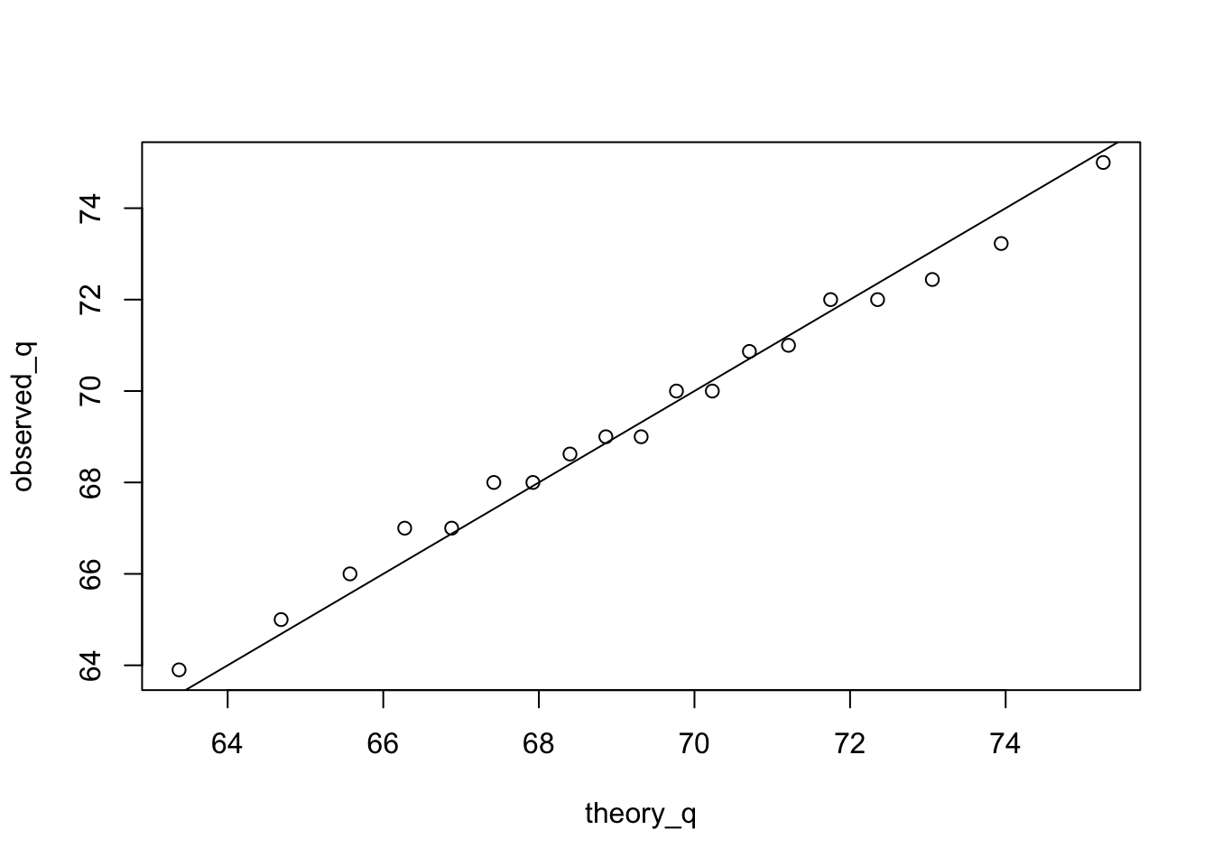
| Version | Author | Date |
|---|---|---|
| 2da8824 | KaranSShakya | 2020-05-20 |
Graph
sessionInfo()R version 4.0.0 (2020-04-24)
Platform: x86_64-apple-darwin17.0 (64-bit)
Running under: macOS Catalina 10.15.4
Matrix products: default
BLAS: /Library/Frameworks/R.framework/Versions/4.0/Resources/lib/libRblas.dylib
LAPACK: /Library/Frameworks/R.framework/Versions/4.0/Resources/lib/libRlapack.dylib
locale:
[1] en_US.UTF-8/en_US.UTF-8/en_US.UTF-8/C/en_US.UTF-8/en_US.UTF-8
attached base packages:
[1] stats graphics grDevices utils datasets methods base
other attached packages:
[1] dslabs_0.7.3 forcats_0.5.0 stringr_1.4.0 dplyr_0.8.5
[5] purrr_0.3.4 readr_1.3.1 tidyr_1.0.3 tibble_3.0.1
[9] ggplot2_3.3.0 tidyverse_1.3.0 workflowr_1.6.2
loaded via a namespace (and not attached):
[1] tidyselect_1.1.0 xfun_0.13 haven_2.2.0 lattice_0.20-41
[5] colorspace_1.4-1 vctrs_0.3.0 generics_0.0.2 htmltools_0.4.0
[9] yaml_2.2.1 utf8_1.1.4 rlang_0.4.6 later_1.0.0
[13] pillar_1.4.4 withr_2.2.0 glue_1.4.1 DBI_1.1.0
[17] dbplyr_1.4.3 modelr_0.1.7 readxl_1.3.1 lifecycle_0.2.0
[21] munsell_0.5.0 gtable_0.3.0 cellranger_1.1.0 rvest_0.3.5
[25] evaluate_0.14 knitr_1.28 httpuv_1.5.2 fansi_0.4.1
[29] broom_0.5.6 Rcpp_1.0.4.6 promises_1.1.0 backports_1.1.6
[33] scales_1.1.1 jsonlite_1.6.1 fs_1.4.1 hms_0.5.3
[37] digest_0.6.25 stringi_1.4.6 grid_4.0.0 rprojroot_1.3-2
[41] cli_2.0.2 tools_4.0.0 magrittr_1.5 crayon_1.3.4
[45] whisker_0.4 pkgconfig_2.0.3 ellipsis_0.3.0 xml2_1.3.2
[49] reprex_0.3.0 lubridate_1.7.8 rstudioapi_0.11 assertthat_0.2.1
[53] rmarkdown_2.1 httr_1.4.1 R6_2.4.1 nlme_3.1-147
[57] git2r_0.27.1 compiler_4.0.0