Population density affects sexual selection in the red flour beetle
Analyses excluding individuals without mating success
Lennart Winkler1, Ronja
Eilhardt1 & Tim Janicke1,2
1Applied Zoology, Technical University Dresden
2Centre d’Écologie Fonctionnelle et Évolutive, UMR 5175,
CNRS, Université de Montpellier
Last updated: 2022-08-13
Checks: 7 0
Knit directory:
Density_and_sexual_selection_2022/
This reproducible R Markdown analysis was created with workflowr (version 1.7.0). The Checks tab describes the reproducibility checks that were applied when the results were created. The Past versions tab lists the development history.
Great! Since the R Markdown file has been committed to the Git repository, you know the exact version of the code that produced these results.
Great job! The global environment was empty. Objects defined in the global environment can affect the analysis in your R Markdown file in unknown ways. For reproduciblity it’s best to always run the code in an empty environment.
The command set.seed(20210613) was run prior to running
the code in the R Markdown file. Setting a seed ensures that any results
that rely on randomness, e.g. subsampling or permutations, are
reproducible.
Great job! Recording the operating system, R version, and package versions is critical for reproducibility.
Nice! There were no cached chunks for this analysis, so you can be confident that you successfully produced the results during this run.
Great job! Using relative paths to the files within your workflowr project makes it easier to run your code on other machines.
Great! You are using Git for version control. Tracking code development and connecting the code version to the results is critical for reproducibility.
The results in this page were generated with repository version f54f022. See the Past versions tab to see a history of the changes made to the R Markdown and HTML files.
Note that you need to be careful to ensure that all relevant files for
the analysis have been committed to Git prior to generating the results
(you can use wflow_publish or
wflow_git_commit). workflowr only checks the R Markdown
file, but you know if there are other scripts or data files that it
depends on. Below is the status of the Git repository when the results
were generated:
Ignored files:
    Ignored:    .Rhistory
    Ignored:    .Rproj.user/

Untracked files:
    Untracked:  analysis/a_start.Rmd
    Untracked:  analysis/index6.Rmd
Note that any generated files, e.g. HTML, png, CSS, etc., are not included in this status report because it is ok for generated content to have uncommitted changes.
These are the previous versions of the repository in which changes were
made to the R Markdown (analysis/index2.Rmd) and HTML
(docs/index2.html) files. If you’ve configured a remote Git
repository (see ?wflow_git_remote), click on the hyperlinks
in the table below to view the files as they were in that past version.
| File | Version | Author | Date | Message |
|---|---|---|---|---|
| Rmd | f54f022 | LennartWinkler | 2022-08-13 | wflow_publish(republish = TRUE, all = T) |
| html | f54f022 | LennartWinkler | 2022-08-13 | wflow_publish(republish = TRUE, all = T) |
| Rmd | f89f7c1 | LennartWinkler | 2022-08-10 | Build site. |
| html | f89f7c1 | LennartWinkler | 2022-08-10 | Build site. |
Supplementary material reporting R code for the manuscript ‘Population density affects sexual selection in the red flour beetle’.
Load and prepare data
Before we started the analyses, we loaded all necessary packages and data.
#load packages
rm(list = ls())
library(ggeffects)
library(ggplot2)
library(gridExtra)
library(lme4)
library(lmerTest)
library(readr)
library(dplyr)
library(EnvStats)
library(cowplot)
library(gridGraphics)
library(car)
library(RColorBrewer)
library(boot)
library(data.table)
library(base)
library(tidyr)
library(ICC)

#load data
DB_data=read_delim("./data/DB_AllData_V04.CSV",";", escape_double = FALSE, trim_ws = TRUE)

#Set factors and level factors
DB_data$Week=as.factor(DB_data$Week)

DB_data$Date=as.factor(DB_data$Date)

DB_data$Sex=as.factor(DB_data$Sex)

DB_data$Gr_size=as.factor(DB_data$Gr_size)
DB_data$Gr_size <- factor(DB_data$Gr_size, levels=c("SG","LG"))

DB_data$Area=as.factor(DB_data$Area)

#Load Body mass data
DB_BM_female <- read_delim("./data/DB_mass_focals_female.CSV",
                           ";", escape_double = FALSE, trim_ws = TRUE)

DB_BM_male <- read_delim("./data/DB_mass_focals_males.CSV",
                         ";", escape_double = FALSE, trim_ws = TRUE)

DB_data_m=merge(DB_data,DB_BM_male,by.x = 'Well_ID',by.y = 'ID_male_focals')
DB_data_f=merge(DB_data,DB_BM_female,by.x = 'F1_ID',by.y = 'ID_female_focals')
DB_data=rbind(DB_data_m,DB_data_f)

###Exclude incomplete data
DB_data=DB_data[DB_data$excluded!=1,]

#Exclude zero MS (all data)####
DB_data=DB_data[DB_data$MatingPartners_number!=0,]

#Calculate total offspring number ####

DB_data$Total_N_MTP1=colSums(rbind(DB_data$N_MTP1_1,DB_data$N_MTP1_2,DB_data$N_MTP1_3,DB_data$N_MTP1_4,DB_data$N_MTP1_5,DB_data$N_MTP1_6), na.rm = T)
DB_data$Total_N_Rd=colSums(rbind(DB_data$N_RD_1,DB_data$N_RD_2,DB_data$N_RD_3,DB_data$N_RD_4,DB_data$N_RD_5,DB_data$N_RD_6), na.rm = T)/DB_data$N_comp

#Calculate proportional RS ####
#Percentage focal offspring
DB_data$m_prop_RS=NA
DB_data$m_prop_RS=(DB_data$Total_N_MTP1/(DB_data$Total_N_MTP1+DB_data$Total_N_Rd))*100
DB_data$m_prop_RS[DB_data$Sex=='F']=NA
DB_data$f_prop_RS=NA
DB_data$f_prop_RS=(DB_data$Total_N_MTP1/(DB_data$Total_N_MTP1+DB_data$Total_N_Rd))*100
DB_data$f_prop_RS[DB_data$Sex=='M']=NA

#Calculate proportion of successful matings ####
DB_data$Prop_MS=NA
DB_data$Prop_MS=DB_data$Matings_number/(DB_data$Attempts_number+DB_data$Matings_number)
DB_data$Prop_MS[DB_data$Prop_MS==0]=NA

#Calculate total encounters ####
DB_data$Total_Encounters=NA
DB_data$Total_Encounters=DB_data$Attempts_number+DB_data$Matings_number

# Treatment identifier for each density ####
n=1
DB_data$Treatment=NA
for(n in 1:length(DB_data$Sex)){if(DB_data$Gr_size[n]=='SG' && DB_data$Area[n]=='Large'){DB_data$Treatment[n]='D = 0.26'
}else if(DB_data$Gr_size[n]=='LG' && DB_data$Area[n]=='Large'){DB_data$Treatment[n]='D = 0.52'
}else if(DB_data$Gr_size[n]=='SG' && DB_data$Area[n]=='Small'){DB_data$Treatment[n]='D = 0.67'
}else if(DB_data$Gr_size[n]=='LG' && DB_data$Area[n]=='Small'){DB_data$Treatment[n]='D = 1.33'
}else{DB_data$Treatment[n]=NA}}

DB_data$Treatment=as.factor(DB_data$Treatment)

# Exclude Incubator 3 data #### -> poor performance
DB_data_clean=DB_data[DB_data$Incu3!=1,]

# Calculate genetic MS ####
# Only clean data
DB_data_clean$gMS=NA
for(i in 1:length(DB_data_clean$Sex)) {if (DB_data_clean$N_MTP1_1[i]>=1 & !is.na (DB_data_clean$N_MTP1_1[i])){
  DB_data_clean$gMS[i]=1
}else{DB_data_clean$gMS[i]=0}}
for(i in 1:length(DB_data_clean$Sex)) {if (DB_data_clean$N_MTP1_2[i]>=1 & !is.na (DB_data_clean$N_MTP1_2[i])){
  DB_data_clean$gMS[i]=DB_data_clean$gMS[i]+1
}else{}}
for(i in 1:length(DB_data_clean$Sex)) {if (DB_data_clean$N_MTP1_3[i]>=1 & !is.na (DB_data_clean$N_MTP1_3[i])){
  DB_data_clean$gMS[i]=DB_data_clean$gMS[i]+1}else{}}
for(i in 1:length(DB_data_clean$Sex)) {if (DB_data_clean$N_MTP1_4[i]>=1 & !is.na (DB_data_clean$N_MTP1_4[i])){
  DB_data_clean$gMS[i]=DB_data_clean$gMS[i]+1}else{}}
for(i in 1:length(DB_data_clean$Sex)) {if (DB_data_clean$N_MTP1_5[i]>=1 & !is.na (DB_data_clean$N_MTP1_5[i])){
  DB_data_clean$gMS[i]=DB_data_clean$gMS[i]+1}else{}}
for(i in 1:length(DB_data_clean$Sex)) {if (DB_data_clean$N_MTP1_6[i]>=1 & !is.na (DB_data_clean$N_MTP1_6[i])){
  DB_data_clean$gMS[i]=DB_data_clean$gMS[i]+1}else{}}

# All data
DB_data$gMS=NA
for(i in 1:length(DB_data$Sex)) {if (DB_data$N_MTP1_1[i]>=1 & !is.na (DB_data$N_MTP1_1[i])){
  DB_data$gMS[i]=1
}else{DB_data$gMS[i]=0}}
for(i in 1:length(DB_data$Sex)) {if (DB_data$N_MTP1_2[i]>=1 & !is.na (DB_data$N_MTP1_2[i])){
  DB_data$gMS[i]=DB_data$gMS[i]+1
}else{}}
for(i in 1:length(DB_data$Sex)) {if (DB_data$N_MTP1_3[i]>=1 & !is.na (DB_data$N_MTP1_3[i])){
  DB_data$gMS[i]=DB_data$gMS[i]+1}else{}}
for(i in 1:length(DB_data$Sex)) {if (DB_data$N_MTP1_4[i]>=1 & !is.na (DB_data$N_MTP1_4[i])){
  DB_data$gMS[i]=DB_data$gMS[i]+1}else{}}
for(i in 1:length(DB_data$Sex)) {if (DB_data$N_MTP1_5[i]>=1 & !is.na (DB_data$N_MTP1_5[i])){
  DB_data$gMS[i]=DB_data$gMS[i]+1}else{}}
for(i in 1:length(DB_data$Sex)) {if (DB_data$N_MTP1_6[i]>=1 & !is.na (DB_data$N_MTP1_6[i])){
  DB_data$gMS[i]=DB_data$gMS[i]+1}else{}}

#Calculate Rd competition RS ####
DB_data_clean$m_RS_Rd_comp=NA
for(i in 1:length(DB_data_clean$Sex)) {if (DB_data_clean$N_MTP1_1[i]>=1 & !is.na (DB_data_clean$N_MTP1_1[i])){
  DB_data_clean$m_RS_Rd_comp[i]=DB_data_clean$N_RD_1[i]
}else{DB_data_clean$m_RS_Rd_comp[i]=0}}
for(i in 1:length(DB_data_clean$Sex)) {if (DB_data_clean$N_MTP1_2[i]>=1 & !is.na (DB_data_clean$N_MTP1_2[i])){
  DB_data_clean$m_RS_Rd_comp[i]=DB_data_clean$m_RS_Rd_comp[i]+DB_data_clean$N_RD_2[i]
}else{}}
for(i in 1:length(DB_data_clean$Sex)) {if (DB_data_clean$N_MTP1_3[i]>=1 & !is.na (DB_data_clean$N_MTP1_3[i])){
  DB_data_clean$m_RS_Rd_comp[i]=DB_data_clean$m_RS_Rd_comp[i]+DB_data_clean$N_RD_3[i]
}else{}}
for(i in 1:length(DB_data_clean$Sex)) {if (DB_data_clean$N_MTP1_4[i]>=1 & !is.na (DB_data_clean$N_MTP1_4[i])){
  DB_data_clean$m_RS_Rd_comp[i]=DB_data_clean$m_RS_Rd_comp[i]+DB_data_clean$N_RD_4[i]
}else{}}
for(i in 1:length(DB_data_clean$Sex)) {if (DB_data_clean$N_MTP1_5[i]>=1 & !is.na (DB_data_clean$N_MTP1_5[i])){
  DB_data_clean$m_RS_Rd_comp[i]=DB_data_clean$m_RS_Rd_comp[i]+DB_data_clean$N_RD_5[i]
}else{}}
for(i in 1:length(DB_data_clean$Sex)) {if (DB_data_clean$N_MTP1_6[i]>=1 & !is.na (DB_data_clean$N_MTP1_6[i])){
  DB_data_clean$m_RS_Rd_comp[i]=DB_data_clean$m_RS_Rd_comp[i]+DB_data_clean$N_RD_6[i]
}else{}}

# Check matings of males #### -> add copulations where offspring found but no copulation registered

for(i in 1:length(DB_data_clean$Sex)) {if (DB_data_clean$N_MTP1_1[i]>=1 && DB_data_clean$Cop_Fe_1[i]==0 & !is.na (DB_data_clean$Cop_Fe_1[i])& !is.na (DB_data_clean$N_MTP1_1[i])){
  DB_data_clean$Cop_Fe_1[i]=1}else{}}
for(i in 1:length(DB_data_clean$Sex)) {if (DB_data_clean$N_MTP1_2[i]>=1 && DB_data_clean$Cop_Fe_2[i]==0 & !is.na (DB_data_clean$Cop_Fe_2[i])& !is.na (DB_data_clean$N_MTP1_2[i])){
  DB_data_clean$Cop_Fe_2[i]=1}else{}}
for(i in 1:length(DB_data_clean$Sex)) {if (DB_data_clean$N_MTP1_3[i]>=1 && DB_data_clean$Cop_Fe_3[i]==0 & !is.na (DB_data_clean$Cop_Fe_3[i])& !is.na (DB_data_clean$N_MTP1_3[i])){
  DB_data_clean$Cop_Fe_3[i]=1}else{}}
for(i in 1:length(DB_data_clean$Sex)) {if (DB_data_clean$N_MTP1_4[i]>=1 && DB_data_clean$Cop_Fe_4[i]==0 & !is.na (DB_data_clean$Cop_Fe_4[i])& !is.na (DB_data_clean$N_MTP1_4[i])){
  DB_data_clean$Cop_Fe_4[i]=1}else{}}
for(i in 1:length(DB_data_clean$Sex)) {if (DB_data_clean$N_MTP1_5[i]>=1 && DB_data_clean$Cop_Fe_5[i]==0 & !is.na (DB_data_clean$Cop_Fe_5[i])& !is.na (DB_data_clean$N_MTP1_5[i])){
  DB_data_clean$Cop_Fe_5[i]=1}else{}}
for(i in 1:length(DB_data_clean$Sex)) {if (DB_data_clean$N_MTP1_6[i]>=1 && DB_data_clean$Cop_Fe_6[i]==0 & !is.na (DB_data_clean$Cop_Fe_6[i])& !is.na (DB_data_clean$N_MTP1_6[i])){
  DB_data_clean$Cop_Fe_6[i]=1}else{}}

# Calculate Rd competition RS of all copulations with potential sperm competition with the  focal ####
DB_data_clean$m_RS_Rd_comp_full=NA
for(i in 1:length(DB_data_clean$Sex)) {if (DB_data_clean$Cop_Fe_1[i]>=1 & !is.na (DB_data_clean$Cop_Fe_1[i])){
  DB_data_clean$m_RS_Rd_comp_full[i]=DB_data_clean$N_RD_1[i]
}else{DB_data_clean$m_RS_Rd_comp_full[i]=0}}
for(i in 1:length(DB_data_clean$Sex)) {if (DB_data_clean$Cop_Fe_2[i]>=1 & !is.na (DB_data_clean$Cop_Fe_2[i])){
  DB_data_clean$m_RS_Rd_comp_full[i]=DB_data_clean$m_RS_Rd_comp_full[i]+DB_data_clean$N_RD_2[i]
}else{}}
for(i in 1:length(DB_data_clean$Sex)) {if (DB_data_clean$Cop_Fe_3[i]>=1 & !is.na (DB_data_clean$Cop_Fe_3[i])){
  DB_data_clean$m_RS_Rd_comp_full[i]=DB_data_clean$m_RS_Rd_comp_full[i]+DB_data_clean$N_RD_3[i]
}else{}}
for(i in 1:length(DB_data_clean$Sex)) {if (DB_data_clean$Cop_Fe_4[i]>=1 & !is.na (DB_data_clean$Cop_Fe_4[i])){
  DB_data_clean$m_RS_Rd_comp_full[i]=DB_data_clean$m_RS_Rd_comp_full[i]+DB_data_clean$N_RD_4[i]
}else{}}
for(i in 1:length(DB_data_clean$Sex)) {if (DB_data_clean$Cop_Fe_5[i]>=1 & !is.na (DB_data_clean$Cop_Fe_5[i])){
  DB_data_clean$m_RS_Rd_comp_full[i]=DB_data_clean$m_RS_Rd_comp_full[i]+DB_data_clean$N_RD_5[i]
}else{}}
for(i in 1:length(DB_data_clean$Sex)) {if (DB_data_clean$Cop_Fe_6[i]>=1 & !is.na (DB_data_clean$Cop_Fe_6[i])){
  DB_data_clean$m_RS_Rd_comp_full[i]=DB_data_clean$m_RS_Rd_comp_full[i]+DB_data_clean$N_RD_6[i]
}else{}}

# Calculate trait values ####
# Males ####
# Total number of matings (all data)
DB_data$m_TotMatings=NA
DB_data$m_TotMatings=DB_data$Matings_number
DB_data$m_TotMatings[DB_data$Sex=='F']=NA

# Avarage mating duration (all data)
DB_data$MatingDuration_av[DB_data$MatingDuration_av==0]=NA
DB_data$m_MatingDuration_av=NA
DB_data$m_MatingDuration_av=DB_data$MatingDuration_av
DB_data$m_MatingDuration_av[DB_data$Sex=='F']=NA
DB_data$MatingDuration_av[DB_data$MatingDuration_av==0]=NA

# Total number of mating attempts (all data)
DB_data$m_Attempts_number=NA
DB_data$m_Attempts_number=DB_data$Attempts_number
DB_data$m_Attempts_number[DB_data$Sex=='F']=NA

# Proportional mating success (all data)
DB_data$m_Prop_MS=NA
DB_data$m_Prop_MS=DB_data$Prop_MS
DB_data$m_Prop_MS[DB_data$Sex=='F']=NA

#Total encounters (all data)
DB_data$m_Total_Encounters=NA
DB_data$m_Total_Encounters=DB_data$Total_Encounters
DB_data$m_Total_Encounters[DB_data$Sex=='F']=NA

# Reproductive success
DB_data_clean$m_RS=NA
DB_data_clean$m_RS=DB_data_clean$Total_N_MTP1
DB_data_clean$m_RS[DB_data_clean$Sex=='F']=NA

# Mating success (number of different partners)
# Clean data
DB_data_clean$m_cMS=NA
DB_data_clean$m_cMS=DB_data_clean$MatingPartners_number
DB_data_clean$m_cMS[DB_data_clean$Sex=='F']=NA
for(i in 1:length(DB_data_clean$m_cMS)) {if (DB_data_clean$gMS[i]>DB_data_clean$m_cMS[i] & !is.na (DB_data_clean$m_cMS[i])){
  DB_data_clean$m_cMS[i]=DB_data_clean$gMS[i]}else{}}

# All data
DB_data$m_cMS=NA
DB_data$m_cMS=DB_data$MatingPartners_number
DB_data$m_cMS[DB_data$Sex=='F']=NA
for(i in 1:length(DB_data$m_cMS)) {if (DB_data$gMS[i]>DB_data$m_cMS[i] & !is.na (DB_data$m_cMS[i])){
  DB_data$m_cMS[i]=DB_data$gMS[i]}else{}}

# Insemination success
DB_data_clean$m_InSuc=NA
DB_data_clean$m_InSuc=DB_data_clean$gMS/DB_data_clean$m_cMS
for(i in 1:length(DB_data_clean$m_InSuc)) {if (DB_data_clean$m_cMS[i]==0 & !is.na (DB_data_clean$m_cMS[i])){
  DB_data_clean$m_InSuc[i]=NA}else{}}

# Fertilization success
DB_data_clean$m_feSuc=NA
DB_data_clean$m_feSuc=DB_data_clean$m_RS/(DB_data_clean$m_RS+DB_data_clean$m_RS_Rd_comp)
for(i in 1:length(DB_data_clean$m_feSuc)) {if (DB_data_clean$m_InSuc[i]==0 | is.na (DB_data_clean$m_InSuc[i])){
  DB_data_clean$m_feSuc[i]=NA}else{}}

# Fecundicty of partners
DB_data_clean$m_pFec=NA
DB_data_clean$m_pFec=(DB_data_clean$m_RS+DB_data_clean$m_RS_Rd_comp)/DB_data_clean$gMS
for(i in 1:length(DB_data_clean$m_pFec)) {if (DB_data_clean$gMS[i]==0){
  DB_data_clean$m_pFec[i]=NA}else{}}

# Paternity success
DB_data_clean$m_PS=NA
DB_data_clean$m_PS=DB_data_clean$m_RS/(DB_data_clean$m_RS+DB_data_clean$m_RS_Rd_comp_full)
for(i in 1:length(DB_data_clean$m_PS)) {if (DB_data_clean$m_RS[i]==0 & !is.na (DB_data_clean$m_RS[i])){
  DB_data_clean$m_PS[i]=NA}else{}}

# Fecundity of partners in all females the focal copulated with
DB_data_clean$m_pFec_compl=NA
DB_data_clean$m_pFec_compl=(DB_data_clean$m_RS+DB_data_clean$m_RS_Rd_comp_full)/DB_data_clean$m_cMS
for(i in 1:length(DB_data_clean$m_pFec)) {if (DB_data_clean$m_cMS[i]==0 & !is.na (DB_data_clean$m_cMS[i])){
  DB_data_clean$m_pFec[i]=NA}else{}}

# Females ####
# Total number of matings (all data)
DB_data$f_TotMatings=NA
DB_data$f_TotMatings=DB_data$Matings_number
DB_data$f_TotMatings[DB_data$Sex=='M']=NA

# Avarage mating duration (all data)
DB_data$f_MatingDuration_av=NA
DB_data$f_MatingDuration_av=DB_data$MatingDuration_av
DB_data$f_MatingDuration_av[DB_data$Sex=='M']=NA
DB_data$MatingDuration_av[DB_data$MatingDuration_av==0]=NA

# Total number of mating attempts (all data)
DB_data$f_Attempts_number=NA
DB_data$f_Attempts_number=DB_data$Attempts_number
DB_data$f_Attempts_number[DB_data$Sex=='M']=NA

# Proportional mating success (all data)
DB_data$f_Prop_MS=NA
DB_data$f_Prop_MS=DB_data$Prop_MS
DB_data_clean$f_Prop_MS[DB_data_clean$Sex=='M']=NA

#Total encounters (all data)
DB_data$f_Total_Encounters=NA
DB_data$f_Total_Encounters=DB_data$Total_Encounters
DB_data$f_Total_Encounters[DB_data$Sex=='M']=NA

# Reproductive success
DB_data_clean$f_RS=NA
DB_data_clean$f_RS=DB_data_clean$Total_N_MTP1
DB_data_clean$f_RS[DB_data_clean$Sex=='M']=NA

# Mating success (number of different partners)
# Clean data
DB_data_clean$f_cMS=NA
DB_data_clean$f_cMS=DB_data_clean$MatingPartners_number
DB_data_clean$f_cMS[DB_data_clean$Sex=='M']=NA
for(i in 1:length(DB_data_clean$f_cMS)) {if (DB_data_clean$gMS[i]>DB_data_clean$f_cMS[i] & !is.na (DB_data_clean$f_cMS[i])){
  DB_data_clean$f_cMS[i]=DB_data_clean$gMS[i]}else{}}

# All data
DB_data$f_cMS=NA
DB_data$f_cMS=DB_data$MatingPartners_number
DB_data$f_cMS[DB_data$Sex=='M']=NA
for(i in 1:length(DB_data$f_cMS)) {if (DB_data$gMS[i]>DB_data$f_cMS[i] & !is.na (DB_data$f_cMS[i])){
  DB_data$f_cMS[i]=DB_data$gMS[i]}else{}}

# Fecundity per mating partner
DB_data_clean$f_fec_pMate=NA
DB_data_clean$f_fec_pMate=DB_data_clean$f_RS/DB_data_clean$f_cMS
for(i in 1:length(DB_data_clean$f_fec_pMate)) {if (DB_data_clean$f_RS[i]==0 & !is.na (DB_data_clean$f_RS[i])){
  DB_data_clean$f_fec_pMate[i]=0}else{}}
for(i in 1:length(DB_data_clean$f_fec_pMate)) {if (DB_data_clean$f_cMS[i]==0 & !is.na (DB_data_clean$f_cMS[i])){
  DB_data_clean$f_fec_pMate[i]=NA}else{}}

# Relativize data per treatment and sex ####
# Small group + large Area
DB_data_clean_0.26=DB_data_clean[DB_data_clean$Treatment=='D = 0.26',]

DB_data_clean_0.26$rel_m_RS=NA
DB_data_clean_0.26$rel_m_prop_RS=NA
DB_data_clean_0.26$rel_m_cMS=NA
DB_data_clean_0.26$rel_m_InSuc=NA
DB_data_clean_0.26$rel_m_feSuc=NA
DB_data_clean_0.26$rel_m_pFec=NA
DB_data_clean_0.26$rel_m_PS=NA
DB_data_clean_0.26$rel_m_pFec_compl=NA

DB_data_clean_0.26$rel_f_RS=NA
DB_data_clean_0.26$rel_f_prop_RS=NA
DB_data_clean_0.26$rel_f_cMS=NA
DB_data_clean_0.26$rel_f_fec_pMate=NA

DB_data_clean_0.26$rel_m_RS=DB_data_clean_0.26$m_RS/mean(DB_data_clean_0.26$m_RS,na.rm=T)
DB_data_clean_0.26$rel_m_prop_RS=DB_data_clean_0.26$m_prop_RS/mean(DB_data_clean_0.26$m_prop_RS,na.rm=T)
DB_data_clean_0.26$rel_m_cMS=DB_data_clean_0.26$m_cMS/mean(DB_data_clean_0.26$m_cMS,na.rm=T)
DB_data_clean_0.26$rel_m_InSuc=DB_data_clean_0.26$m_InSuc/mean(DB_data_clean_0.26$m_InSuc,na.rm=T)
DB_data_clean_0.26$rel_m_feSuc=DB_data_clean_0.26$m_feSuc/mean(DB_data_clean_0.26$m_feSuc,na.rm=T)
DB_data_clean_0.26$rel_m_pFec=DB_data_clean_0.26$m_pFec/mean(DB_data_clean_0.26$m_pFec,na.rm=T)
DB_data_clean_0.26$rel_m_PS=DB_data_clean_0.26$m_PS/mean(DB_data_clean_0.26$m_PS,na.rm=T)
DB_data_clean_0.26$rel_m_pFec_compl=DB_data_clean_0.26$m_pFec_compl/mean(DB_data_clean_0.26$m_pFec_compl,na.rm=T)

DB_data_clean_0.26$rel_f_RS=DB_data_clean_0.26$f_RS/mean(DB_data_clean_0.26$f_RS,na.rm=T)
DB_data_clean_0.26$rel_f_prop_RS=DB_data_clean_0.26$f_prop_RS/mean(DB_data_clean_0.26$f_prop_RS,na.rm=T)
DB_data_clean_0.26$rel_f_cMS=DB_data_clean_0.26$f_cMS/mean(DB_data_clean_0.26$f_cMS,na.rm=T)
DB_data_clean_0.26$rel_f_fec_pMate=DB_data_clean_0.26$f_fec_pMate/mean(DB_data_clean_0.26$f_fec_pMate,na.rm=T)

# Large group + large Area
DB_data_clean_0.52=DB_data_clean[DB_data_clean$Treatment=='D = 0.52',]
#Relativize data

DB_data_clean_0.52$rel_m_RS=NA
DB_data_clean_0.52$rel_m_prop_RS=NA
DB_data_clean_0.52$rel_m_cMS=NA
DB_data_clean_0.52$rel_m_InSuc=NA
DB_data_clean_0.52$rel_m_feSuc=NA
DB_data_clean_0.52$rel_m_pFec=NA
DB_data_clean_0.52$rel_m_PS=NA
DB_data_clean_0.52$rel_m_pFec_compl=NA

DB_data_clean_0.52$rel_f_RS=NA
DB_data_clean_0.52$rel_f_prop_RS=NA
DB_data_clean_0.52$rel_f_cMS=NA
DB_data_clean_0.52$rel_f_fec_pMate=NA

DB_data_clean_0.52$rel_m_RS=DB_data_clean_0.52$m_RS/mean(DB_data_clean_0.52$m_RS,na.rm=T)
DB_data_clean_0.52$rel_m_prop_RS=DB_data_clean_0.52$m_prop_RS/mean(DB_data_clean_0.52$m_prop_RS,na.rm=T)
DB_data_clean_0.52$rel_m_cMS=DB_data_clean_0.52$m_cMS/mean(DB_data_clean_0.52$m_cMS,na.rm=T)
DB_data_clean_0.52$rel_m_InSuc=DB_data_clean_0.52$m_InSuc/mean(DB_data_clean_0.52$m_InSuc,na.rm=T)
DB_data_clean_0.52$rel_m_feSuc=DB_data_clean_0.52$m_feSuc/mean(DB_data_clean_0.52$m_feSuc,na.rm=T)
DB_data_clean_0.52$rel_m_pFec=DB_data_clean_0.52$m_pFec/mean(DB_data_clean_0.52$m_pFec,na.rm=T)
DB_data_clean_0.52$rel_m_PS=DB_data_clean_0.52$m_PS/mean(DB_data_clean_0.52$m_PS,na.rm=T)
DB_data_clean_0.52$rel_m_pFec_compl=DB_data_clean_0.52$m_pFec_compl/mean(DB_data_clean_0.52$m_pFec_compl,na.rm=T)

DB_data_clean_0.52$rel_f_RS=DB_data_clean_0.52$f_RS/mean(DB_data_clean_0.52$f_RS,na.rm=T)
DB_data_clean_0.52$rel_f_prop_RS=DB_data_clean_0.52$f_prop_RS/mean(DB_data_clean_0.52$f_prop_RS,na.rm=T)
DB_data_clean_0.52$rel_f_cMS=DB_data_clean_0.52$f_cMS/mean(DB_data_clean_0.52$f_cMS,na.rm=T)
DB_data_clean_0.52$rel_f_fec_pMate=DB_data_clean_0.52$f_fec_pMate/mean(DB_data_clean_0.52$f_fec_pMate,na.rm=T)

# Small group + small Area
DB_data_clean_0.67=DB_data_clean[DB_data_clean$Treatment=='D = 0.67',]
#Relativize data
DB_data_clean_0.67$rel_m_RS=NA
DB_data_clean_0.67$rel_m_prop_RS=NA
DB_data_clean_0.67$rel_m_cMS=NA
DB_data_clean_0.67$rel_m_InSuc=NA
DB_data_clean_0.67$rel_m_feSuc=NA
DB_data_clean_0.67$rel_m_pFec=NA
DB_data_clean_0.67$rel_m_PS=NA
DB_data_clean_0.67$rel_m_pFec_compl=NA

DB_data_clean_0.67$rel_f_RS=NA
DB_data_clean_0.67$rel_f_prop_RS=NA
DB_data_clean_0.67$rel_f_cMS=NA
DB_data_clean_0.67$rel_f_fec_pMate=NA

DB_data_clean_0.67$rel_m_RS=DB_data_clean_0.67$m_RS/mean(DB_data_clean_0.67$m_RS,na.rm=T)
DB_data_clean_0.67$rel_m_prop_RS=DB_data_clean_0.67$m_prop_RS/mean(DB_data_clean_0.67$m_prop_RS,na.rm=T)
DB_data_clean_0.67$rel_m_cMS=DB_data_clean_0.67$m_cMS/mean(DB_data_clean_0.67$m_cMS,na.rm=T)
DB_data_clean_0.67$rel_m_InSuc=DB_data_clean_0.67$m_InSuc/mean(DB_data_clean_0.67$m_InSuc,na.rm=T)
DB_data_clean_0.67$rel_m_feSuc=DB_data_clean_0.67$m_feSuc/mean(DB_data_clean_0.67$m_feSuc,na.rm=T)
DB_data_clean_0.67$rel_m_pFec=DB_data_clean_0.67$m_pFec/mean(DB_data_clean_0.67$m_pFec,na.rm=T)
DB_data_clean_0.67$rel_m_PS=DB_data_clean_0.67$m_PS/mean(DB_data_clean_0.67$m_PS,na.rm=T)
DB_data_clean_0.67$rel_m_pFec_compl=DB_data_clean_0.67$m_pFec_compl/mean(DB_data_clean_0.67$m_pFec_compl,na.rm=T)

DB_data_clean_0.67$rel_f_RS=DB_data_clean_0.67$f_RS/mean(DB_data_clean_0.67$f_RS,na.rm=T)
DB_data_clean_0.67$rel_f_prop_RS=DB_data_clean_0.67$f_prop_RS/mean(DB_data_clean_0.67$f_prop_RS,na.rm=T)
DB_data_clean_0.67$rel_f_cMS=DB_data_clean_0.67$f_cMS/mean(DB_data_clean_0.67$f_cMS,na.rm=T)
DB_data_clean_0.67$rel_f_fec_pMate=DB_data_clean_0.67$f_fec_pMate/mean(DB_data_clean_0.67$f_fec_pMate,na.rm=T)

# Large group + small Area
DB_data_clean_1.33=DB_data_clean[DB_data_clean$Treatment=='D = 1.33',]
#Relativize data

DB_data_clean_1.33$rel_m_RS=NA
DB_data_clean_1.33$rel_m_prop_RS=NA
DB_data_clean_1.33$rel_m_cMS=NA
DB_data_clean_1.33$rel_m_InSuc=NA
DB_data_clean_1.33$rel_m_feSuc=NA
DB_data_clean_1.33$rel_m_pFec=NA
DB_data_clean_1.33$rel_m_PS=NA
DB_data_clean_1.33$rel_m_pFec_compl=NA

DB_data_clean_1.33$rel_f_RS=NA
DB_data_clean_1.33$rel_f_prop_RS=NA
DB_data_clean_1.33$rel_f_cMS=NA
DB_data_clean_1.33$rel_f_fec_pMate=NA

DB_data_clean_1.33$rel_m_RS=DB_data_clean_1.33$m_RS/mean(DB_data_clean_1.33$m_RS,na.rm=T)
DB_data_clean_1.33$rel_m_prop_RS=DB_data_clean_1.33$m_prop_RS/mean(DB_data_clean_1.33$m_prop_RS,na.rm=T)
DB_data_clean_1.33$rel_m_cMS=DB_data_clean_1.33$m_cMS/mean(DB_data_clean_1.33$m_cMS,na.rm=T)
DB_data_clean_1.33$rel_m_InSuc=DB_data_clean_1.33$m_InSuc/mean(DB_data_clean_1.33$m_InSuc,na.rm=T)
DB_data_clean_1.33$rel_m_feSuc=DB_data_clean_1.33$m_feSuc/mean(DB_data_clean_1.33$m_feSuc,na.rm=T)
DB_data_clean_1.33$rel_m_pFec=DB_data_clean_1.33$m_pFec/mean(DB_data_clean_1.33$m_pFec,na.rm=T)
DB_data_clean_1.33$rel_m_PS=DB_data_clean_1.33$m_PS/mean(DB_data_clean_1.33$m_PS,na.rm=T)
DB_data_clean_1.33$rel_m_pFec_compl=DB_data_clean_1.33$m_pFec_compl/mean(DB_data_clean_1.33$m_pFec_compl,na.rm=T)

DB_data_clean_1.33$rel_f_RS=DB_data_clean_1.33$f_RS/mean(DB_data_clean_1.33$f_RS,na.rm=T)
DB_data_clean_1.33$rel_f_prop_RS=DB_data_clean_1.33$f_prop_RS/mean(DB_data_clean_1.33$f_prop_RS,na.rm=T)
DB_data_clean_1.33$rel_f_cMS=DB_data_clean_1.33$f_cMS/mean(DB_data_clean_1.33$f_cMS,na.rm=T)
DB_data_clean_1.33$rel_f_fec_pMate=DB_data_clean_1.33$f_fec_pMate/mean(DB_data_clean_1.33$f_fec_pMate,na.rm=T)

# Set colors for figures
colpal=brewer.pal(4, 'Dark2')
colpal2=brewer.pal(3, 'Set1')
colpal3=brewer.pal(4, 'Paired')
slava_ukrajini=(c('#0057B8','#FFD700'))
colorESEB=c('#01519c','#ffdf33')
colorESEB2=c('#1DA1F2','#ffec69')

# Merge data according to treatment #### -> Reduce treatments to area and population size
#Area
DB_data_clean_Large_area=rbind(DB_data_clean_0.26,DB_data_clean_0.52)
DB_data_clean_Small_area=rbind(DB_data_clean_0.67,DB_data_clean_1.33)

#Population size
DB_data_clean_Small_pop=rbind(DB_data_clean_0.26,DB_data_clean_0.67)
DB_data_clean_Large_pop=rbind(DB_data_clean_0.52,DB_data_clean_1.33)

# Merge data according to treatment full data set #### -> Reduce treatments to area and population size
DB_data_0.26=DB_data[DB_data$Treatment=='D = 0.26',]
DB_data_0.52=DB_data[DB_data$Treatment=='D = 0.52',]
DB_data_0.67=DB_data[DB_data$Treatment=='D = 0.67',]
DB_data_1.33=DB_data[DB_data$Treatment=='D = 1.33',]

#Area
DB_data_Large_area_full=rbind(DB_data_0.26,DB_data_0.52)
DB_data_Small_area_full=rbind(DB_data_0.67,DB_data_1.33)

#Population size
DB_data_Small_pop_full=rbind(DB_data_0.26,DB_data_0.67)
DB_data_Large_pop_full=rbind(DB_data_0.52,DB_data_1.33)
Treatment effects
Mating behaviour
We first tested the effect that the treatments (group size and area)
had on the mating behaviour of focal beetles.
Behavioural
variables:
- Number of matings
- Number of different mating
partners (mating success)
- Mating duration in seconds
- Mating
encounters (mating number + mating attempts)
- Proportion of
successful matings (mating number/mating number + mating attempts)
Number of matings
# Figure: Number of matings
# Treatment: Group size
p1<-ggplot(DB_data, aes(x=Sex, y=as.numeric(Matings_number),fill=Gr_size, col=Gr_size)) +
geom_point(position=position_jitterdodge(jitter.width=0.6,jitter.height = 0,dodge.width=0.9),shape=19, alpha=0.75, size = 2)+
stat_summary(fun.min = function(z) { quantile(z,0.25) },
fun.max = function(z) { quantile(z,0.75) },
fun = mean,position=position_dodge(.9), size = 0.9,col='black',show.legend = F)+
scale_color_manual(values=c(colorESEB[1],colorESEB[2]),name = "Treatment", labels = c('Small group','Large group'))+
scale_fill_manual(values=c(colorESEB[1],colorESEB[2]),name = "Treatment", labels = c('Small group','Large group'))+
xlab('Sex')+ylab("Number of matings")+ggtitle('')+ theme(plot.title = element_text(hjust = 0.5))+
scale_x_discrete(labels = c('Female','Male'),drop=FALSE)+ ylim(0,12)+labs(tag = "A")+
annotate("text",label='n =',x=0.55,y=12,size=4)+
annotate("text",label='91',x=0.78,y=12,size=4)+
annotate("text",label='74',x=1.23,y=12,size=4)+
annotate("text",label='85',x=1.78,y=12,size=4)+
annotate("text",label='85',x=2.23,y=12,size=4)+
theme(panel.border = element_blank(),
plot.margin = margin(0.15,2.2,0,0.2,"cm"),
plot.title = element_text(hjust = 0.5),
panel.background = element_blank(),
legend.key=element_blank(),
panel.grid.major = element_blank(),
panel.grid.minor = element_blank(),
legend.position = c(1.08, 0.8),
plot.tag.position=c(0.01,0.98),
legend.title = element_blank(),
legend.text = element_text(colour="black", size=10),
axis.line.x = element_line(colour = "black", size = 1),
axis.line.y = element_line(colour = "black", size = 1),
axis.text.x = element_text(face="plain", color="black", size=16, angle=0),
axis.text.y = element_text(face="plain", color="black", size=16, angle=0),
axis.title.x = element_text(size=16,face="plain", margin = margin(r=0,10,0,0)),
axis.title.y = element_text(size=16,face="plain", margin = margin(r=10,0,0,0)),
axis.ticks = element_line(size = 1),
axis.ticks.length = unit(.3, "cm"))+
guides(colour = guide_legend(override.aes = list(size=4)))
# Treatment: Area
p1.2<-ggplot(DB_data, aes(x=Sex, y=as.numeric(Matings_number),fill=Area, col=Area)) +
geom_point(position=position_jitterdodge(jitter.width=0.6,jitter.height = 0,dodge.width=0.9),shape=19, alpha=0.75, size = 2)+
stat_summary(fun.min = function(z) { quantile(z,0.25) },
fun.max = function(z) { quantile(z,0.75) },
fun = mean,position=position_dodge(.9), size = 0.9,col='black',show.legend = F)+
scale_color_manual(values=c(colorESEB2[1],colorESEB2[2]),name = "Treatment", labels = c('Large area','Small area'))+
scale_fill_manual(values=c(colorESEB2[1],colorESEB2[2]),name = "Treatment", labels = c('Large area','Small area'))+
xlab('Sex')+ylab("")+ggtitle('')+ theme(plot.title = element_text(hjust = 0.5))+labs(tag = "B")+
scale_x_discrete(labels = c('Female','Male'),drop=FALSE)+ ylim(0,12)+
annotate("text",label='n =',x=0.55,y=12,size=4)+
annotate("text",label='86',x=0.78,y=12,size=4)+
annotate("text",label='79',x=1.23,y=12,size=4)+
annotate("text",label='88',x=1.78,y=12,size=4)+
annotate("text",label='82',x=2.23,y=12,size=4)+
theme(panel.border = element_blank(),
plot.margin = margin(0.15,2.2,0,0,"cm"),
plot.title = element_text(hjust = 0.5),
panel.background = element_blank(),
legend.key=element_blank(),
panel.grid.major = element_blank(),
panel.grid.minor = element_blank(),
legend.position = c(1.08, 0.8),
plot.tag.position=c(0.01,0.98),
legend.title = element_blank(),
legend.text = element_text(colour="black", size=10),
axis.line.x = element_line(colour = "black", size = 1),
axis.line.y = element_line(colour = "black", size = 1),
axis.text.x = element_text(face="plain", color="black", size=16, angle=0),
axis.text.y = element_text(face="plain", color="black", size=16, angle=0),
axis.title.x = element_text(size=16,face="plain", margin = margin(r=0,10,0,0)),
axis.title.y = element_text(size=16,face="plain", margin = margin(r=10,0,0,0)),
axis.ticks = element_line(size = 1),
axis.ticks.length = unit(.3, "cm"))+
guides(colour = guide_legend(override.aes = list(size=4)))
grid.arrange(grobs = list(p1,p1.2), nrow = 1,ncol=2, widths=c(2.3, 2.3))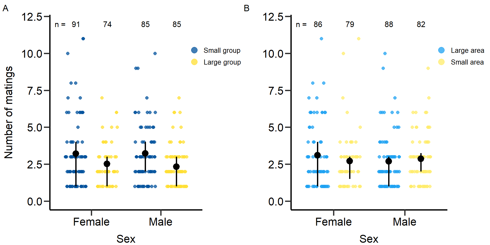 Figure 1: Effects of group size (A) and area treatment (B) on the number
of matings of female and male focals. Black bars indicate means and
standard errors.
Figure 1: Effects of group size (A) and area treatment (B) on the number
of matings of female and male focals. Black bars indicate means and
standard errors.
Statistical models: Number of matings (quasi-Poisson
GLM)
Effect of group size on number of matings in females.
mod1.1=glm(f_TotMatings~Gr_size,data=DB_data,family = quasipoisson)
summary(mod1.1)
Call:
glm(formula = f_TotMatings ~ Gr_size, family = quasipoisson,
    data = DB_data)

Deviance Residuals:
    Min       1Q   Median       3Q      Max
-1.4425  -1.0911  -0.3395   0.3940   3.3970

Coefficients:
            Estimate Std. Error t value Pr(>|t|)
(Intercept)  1.16475    0.07523  15.483   <2e-16 ***
Gr_sizeLG   -0.24080    0.12830  -1.877   0.0628 .
---
Signif. codes:  0 '***' 0.001 '**' 0.01 '*' 0.05 '.' 0.1 ' ' 1

(Dispersion parameter for quasipoisson family taken to be 1.41487)

    Null deviance: 164.51  on 129  degrees of freedom
Residual deviance: 159.41  on 128  degrees of freedom
  (148 Beobachtungen als fehlend gelöscht)
AIC: NA

Number of Fisher Scoring iterations: 5
Effect of group size on number of matings in males.
# Sex: Male
# Treatment: Group size
mod1.2=glm(m_TotMatings~Gr_size,data=DB_data,family = quasipoisson)
summary(mod1.2)
Call:
glm(formula = m_TotMatings ~ Gr_size, family = quasipoisson,
    data = DB_data)

Deviance Residuals:
    Min       1Q   Median       3Q      Max
-1.4492  -0.9859  -0.2238   0.4178   3.0179

Coefficients:
            Estimate Std. Error t value Pr(>|t|)
(Intercept)  1.16913    0.06702  17.445  < 2e-16 ***
Gr_sizeLG   -0.32183    0.10258  -3.137  0.00206 **
---
Signif. codes:  0 '***' 0.001 '**' 0.01 '*' 0.05 '.' 0.1 ' ' 1

(Dispersion parameter for quasipoisson family taken to be 1.055494)

    Null deviance: 150.57  on 147  degrees of freedom
Residual deviance: 140.06  on 146  degrees of freedom
  (130 Beobachtungen als fehlend gelöscht)
AIC: NA

Number of Fisher Scoring iterations: 5
Effect of area on number of matings in females.
# Sex: Female
# Treatment: Area
mod1.3=glm(f_TotMatings~Area,data=DB_data,family = quasipoisson)
summary(mod1.3)
Call:
glm(formula = f_TotMatings ~ Area, family = quasipoisson, data = DB_data)

Deviance Residuals:
    Min       1Q   Median       3Q      Max
-1.3980  -1.1952  -0.4536   0.4041   3.7722

Coefficients:
            Estimate Std. Error t value Pr(>|t|)
(Intercept)  1.13548    0.08198   13.85   <2e-16 ***
AreaSmall   -0.13785    0.12650   -1.09    0.278
---
Signif. codes:  0 '***' 0.001 '**' 0.01 '*' 0.05 '.' 0.1 ' ' 1

(Dispersion parameter for quasipoisson family taken to be 1.485185)

    Null deviance: 164.51  on 129  degrees of freedom
Residual deviance: 162.74  on 128  degrees of freedom
  (148 Beobachtungen als fehlend gelöscht)
AIC: NA

Number of Fisher Scoring iterations: 5
Effect of area on number of matings in males.
# Sex: Male
# Treatment: Area
mod1.4=glm(m_TotMatings~Area,data=DB_data,family = quasipoisson)
summary(mod1.4)
Call:
glm(formula = m_TotMatings ~ Area, family = quasipoisson, data = DB_data)

Deviance Residuals:
    Min       1Q   Median       3Q      Max
-1.2727  -1.1805  -0.4376   0.1891   3.4165

Coefficients:
            Estimate Std. Error t value Pr(>|t|)
(Intercept)  0.98739    0.07560  13.061   <2e-16 ***
AreaSmall    0.06382    0.10665   0.598     0.55
---
Signif. codes:  0 '***' 0.001 '**' 0.01 '*' 0.05 '.' 0.1 ' ' 1

(Dispersion parameter for quasipoisson family taken to be 1.165813)

    Null deviance: 150.57  on 147  degrees of freedom
Residual deviance: 150.15  on 146  degrees of freedom
  (130 Beobachtungen als fehlend gelöscht)
AIC: NA

Number of Fisher Scoring iterations: 5
Number of mating partners
# Figure: Number of mating partners (mating success)
# Treatment: Group size
p2<-ggplot(DB_data, aes(x=Sex, y=as.numeric(MatingPartners_number),fill=Gr_size, col=Gr_size)) +
geom_point(position=position_jitterdodge(jitter.width=0.6,jitter.height = 0,dodge.width=0.9),shape=19, alpha=0.75, size = 2)+
stat_summary(fun.min = function(z) { quantile(z,0.25) },
fun.max = function(z) { quantile(z,0.75) },
fun = mean,position=position_dodge(.9), size = 0.9,col='black',show.legend = F)+
scale_color_manual(values=c(colorESEB[1],colorESEB[2]),name = "Treatment", labels = c('Small group','Large group'))+
scale_fill_manual(values=c(colorESEB[1],colorESEB[2]),name = "Treatment", labels = c('Small group','Large group'))+
xlab('Sex')+ylab("Number of partners")+ggtitle('')+ theme(plot.title = element_text(hjust = 0.5))+
scale_x_discrete(labels = c('Female','Male'),drop=FALSE)+ ylim(0,5.4)+labs(tag = "A")+
annotate("text",label='n =',x=0.55,y=5.4,size=4)+
annotate("text",label='91',x=0.78,y=5.4,size=4)+
annotate("text",label='74',x=1.23,y=5.4,size=4)+
annotate("text",label='85',x=1.78,y=5.4,size=4)+
annotate("text",label='85',x=2.23,y=5.4,size=4)+
theme(panel.border = element_blank(),
plot.margin = margin(0,2.2,0,0.2,"cm"),
plot.title = element_text(hjust = 0.5),
panel.background = element_blank(),
legend.key=element_blank(),
panel.grid.major = element_blank(),
panel.grid.minor = element_blank(),
legend.position = c(1.08, 0.8),
plot.tag.position=c(0.01,0.98),
legend.title = element_blank(),
legend.text = element_text(colour="black", size=10),
axis.line.x = element_line(colour = "black", size = 1),
axis.line.y = element_line(colour = "black", size = 1),
axis.text.x = element_text(face="plain", color="black", size=16, angle=0),
axis.text.y = element_text(face="plain", color="black", size=16, angle=0),
axis.title.x = element_text(size=16,face="plain", margin = margin(r=0,10,0,0)),
axis.title.y = element_text(size=16,face="plain", margin = margin(r=10,0,0,0)),
axis.ticks = element_line(size = 1),
axis.ticks.length = unit(.3, "cm"))+
guides(colour = guide_legend(override.aes = list(size=4)))
# Treatment: Area
p2.2<-ggplot(DB_data, aes(x=Sex, y=as.numeric(MatingPartners_number),fill=Area, col=Area)) +
geom_point(position=position_jitterdodge(jitter.width=0.6,jitter.height = 0,dodge.width=0.9),shape=19, alpha=0.75, size = 2)+
stat_summary(fun.min = function(z) { quantile(z,0.25) },
fun.max = function(z) { quantile(z,0.75) },
fun = mean,position=position_dodge(.9), size = 0.9,col='black',show.legend = F)+
scale_color_manual(values=c(colorESEB2[1],colorESEB2[2]),name = "Treatment", labels = c('Large area','Small area'))+
scale_fill_manual(values=c(colorESEB2[1],colorESEB2[2]),name = "Treatment", labels = c('Large area','Small area'))+
xlab('Sex')+ylab("")+ggtitle('')+ theme(plot.title = element_text(hjust = 0.5))+
scale_x_discrete(labels = c('Female','Male'),drop=FALSE)+ ylim(0,5.4)+labs(tag = "B")+
annotate("text",label='n =',x=0.55,y=5.4,size=4)+
annotate("text",label='86',x=0.78,y=5.4,size=4)+
annotate("text",label='79',x=1.23,y=5.4,size=4)+
annotate("text",label='88',x=1.78,y=5.4,size=4)+
annotate("text",label='82',x=2.23,y=5.4,size=4)+
theme(panel.border = element_blank(),
plot.margin = margin(0,2.2,0,0,"cm"),
plot.title = element_text(hjust = 0.5),
panel.background = element_blank(),
legend.key=element_blank(),
panel.grid.major = element_blank(),
panel.grid.minor = element_blank(),
legend.position = c(1.08, 0.8),
plot.tag.position=c(0.01,0.98),
legend.title = element_blank(),
legend.text = element_text(colour="black", size=10),
axis.line.x = element_line(colour = "black", size = 1),
axis.line.y = element_line(colour = "black", size = 1),
axis.text.x = element_text(face="plain", color="black", size=16, angle=0),
axis.text.y = element_text(face="plain", color="black", size=16, angle=0),
axis.title.x = element_text(size=16,face="plain", margin = margin(r=0,10,0,0)),
axis.title.y = element_text(size=16,face="plain", margin = margin(r=10,0,0,0)),
axis.ticks = element_line(size = 1),
axis.ticks.length = unit(.3, "cm"))+
guides(colour = guide_legend(override.aes = list(size=4)))
plot2<-grid.arrange(grobs = list(p2,p2.2), nrow = 1,ncol=2, widths=c(2.3, 2.3))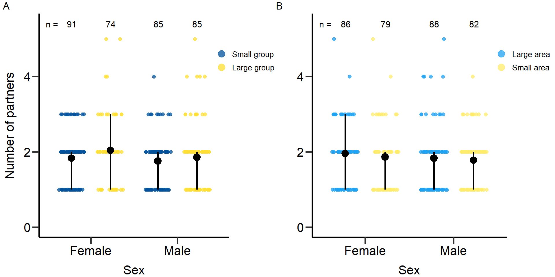 Figure 2: Effects of group size (A) and area treatment (B) on the number
of mating partners of female and male focals. Black bars indicate means
and quartile borders.
Figure 2: Effects of group size (A) and area treatment (B) on the number
of mating partners of female and male focals. Black bars indicate means
and quartile borders.
Statistical models: Number of mating partners (quasi-Poisson
GLM)
Effect of group size on number of mating partners in
females.
# Statistical models: Number of mating partners (quasi-Poisson GLM)
# Sex: Female
# Treatment: Group size
mod2.1=glm(f_cMS~Gr_size,data=DB_data,family = quasipoisson)
summary(mod2.1)
Call:
glm(formula = f_cMS ~ Gr_size, family = quasipoisson, data = DB_data)

Deviance Residuals:
     Min        1Q    Median        3Q       Max
-0.80779  -0.67409   0.04713   0.12129   1.74624

Coefficients:
            Estimate Std. Error t value Pr(>|t|)
(Intercept)  0.60614    0.05211  11.631   <2e-16 ***
Gr_sizeLG    0.10606    0.07987   1.328    0.187
---
Signif. codes:  0 '***' 0.001 '**' 0.01 '*' 0.05 '.' 0.1 ' ' 1

(Dispersion parameter for quasipoisson family taken to be 0.3883379)

    Null deviance: 49.041  on 129  degrees of freedom
Residual deviance: 48.360  on 128  degrees of freedom
  (148 Beobachtungen als fehlend gelöscht)
AIC: NA

Number of Fisher Scoring iterations: 4
Effect of group size on number of mating partners in males.
# Sex: Male
# Treatment: Group size
mod2.2=glm(m_cMS~Gr_size,data=DB_data,family = quasipoisson)
summary(mod2.2)
Call:
glm(formula = m_cMS ~ Gr_size, family = quasipoisson, data = DB_data)

Deviance Residuals:
     Min        1Q    Median        3Q       Max
-0.69644  -0.61944   0.09646   0.18208   1.89372

Coefficients:
            Estimate Std. Error t value Pr(>|t|)
(Intercept)  0.56157    0.05425  10.352   <2e-16 ***
Gr_sizeLG    0.06258    0.07505   0.834    0.406
---
Signif. codes:  0 '***' 0.001 '**' 0.01 '*' 0.05 '.' 0.1 ' ' 1

(Dispersion parameter for quasipoisson family taken to be 0.3766698)

    Null deviance: 52.151  on 147  degrees of freedom
Residual deviance: 51.889  on 146  degrees of freedom
  (130 Beobachtungen als fehlend gelöscht)
AIC: NA

Number of Fisher Scoring iterations: 4
Effect of area on number of mating partners in females.
# Sex: Female
# Treatment: Area
mod2.3=glm(f_cMS~Area,data=DB_data,family = quasipoisson)
summary(mod2.3)
Call:
glm(formula = f_cMS ~ Area, family = quasipoisson, data = DB_data)

Deviance Residuals:
     Min        1Q    Median        3Q       Max
-0.75624  -0.69493   0.03009   0.09814   1.89572

Coefficients:
            Estimate Std. Error t value Pr(>|t|)
(Intercept)  0.67179    0.05356  12.542   <2e-16 ***
AreaSmall   -0.04885    0.08059  -0.606    0.545
---
Signif. codes:  0 '***' 0.001 '**' 0.01 '*' 0.05 '.' 0.1 ' ' 1

(Dispersion parameter for quasipoisson family taken to be 0.3988074)

    Null deviance: 49.041  on 129  degrees of freedom
Residual deviance: 48.894  on 128  degrees of freedom
  (148 Beobachtungen als fehlend gelöscht)
AIC: NA

Number of Fisher Scoring iterations: 4
Effect of area on number of mating partners in males.
# Sex: Male
# Treatment: Area
mod2.4=glm(m_cMS~Area,data=DB_data,family = quasipoisson)
summary(mod2.4)
Call:
glm(formula = m_cMS ~ Area, family = quasipoisson, data = DB_data)

Deviance Residuals:
    Min       1Q   Median       3Q      Max
-0.6711  -0.6458   0.1246   0.1528   1.9274

Coefficients:
            Estimate Std. Error t value Pr(>|t|)
(Intercept)  0.60374    0.05228  11.549   <2e-16 ***
AreaSmall   -0.02059    0.07535  -0.273    0.785
---
Signif. codes:  0 '***' 0.001 '**' 0.01 '*' 0.05 '.' 0.1 ' ' 1

(Dispersion parameter for quasipoisson family taken to be 0.379889)

    Null deviance: 52.151  on 147  degrees of freedom
Residual deviance: 52.123  on 146  degrees of freedom
  (130 Beobachtungen als fehlend gelöscht)
AIC: NA

Number of Fisher Scoring iterations: 4
Mating duration
#Figure: Mating duration in seconds
# Treatment: Group size
p3<-ggplot(DB_data, aes(x=Sex, y=as.numeric(MatingDuration_av),fill=Gr_size, col=Gr_size)) +
geom_point(position=position_jitterdodge(jitter.width=0.6,jitter.height = 0,dodge.width=0.9),shape=19, alpha=0.75, size = 2)+
stat_summary(fun.min = function(z) { quantile(z,0.25) },
fun.max = function(z) { quantile(z,0.75) },
fun = mean,position=position_dodge(.9), size = 0.9,col='black',show.legend = F)+
scale_color_manual(values=c(colorESEB[1],colorESEB[2]),name = "Treatment", labels = c('Small group','Large group'))+
scale_fill_manual(values=c(colorESEB[1],colorESEB[2]),name = "Treatment", labels = c('Small group','Large group'))+
xlab('Sex')+ylab("Mean mating duration")+ggtitle('')+ theme(plot.title = element_text(hjust = 0.5))+
scale_x_discrete(labels = c('Female','Male'),drop=FALSE)+ ylim(0,390)+labs(tag = "A")+
annotate("text",label='n =',x=0.55,y=390,size=4)+
annotate("text",label='91',x=0.78,y=390,size=4)+
annotate("text",label='74',x=1.23,y=390,size=4)+
annotate("text",label='85',x=1.78,y=390,size=4)+
annotate("text",label='85',x=2.23,y=390,size=4)+
theme(panel.border = element_blank(),
plot.margin = margin(0,2.2,0.15,0.2,"cm"),
plot.title = element_text(hjust = 0.5),
panel.background = element_blank(),
legend.key=element_blank(),
panel.grid.major = element_blank(),
panel.grid.minor = element_blank(),
legend.position = c(1.08, 0.8),
plot.tag.position=c(0.01,0.98),
legend.title = element_blank(),
legend.text = element_text(colour="black", size=10),
axis.line.x = element_line(colour = "black", size = 1),
axis.line.y = element_line(colour = "black", size = 1),
axis.text.x = element_text(face="plain", color="black", size=16, angle=0),
axis.text.y = element_text(face="plain", color="black", size=16, angle=0),
axis.title.x = element_text(size=16,face="plain", margin = margin(r=0,10,0,0)),
axis.title.y = element_text(size=16,face="plain", margin = margin(r=10,0,0,0)),
axis.ticks = element_line(size = 1),
axis.ticks.length = unit(.3, "cm"))+
guides(colour = guide_legend(override.aes = list(size=4)))
# Treatment: Area
p3.2<-ggplot(DB_data, aes(x=Sex, y=as.numeric(MatingDuration_av),fill=Area, col=Area)) +
geom_point(position=position_jitterdodge(jitter.width=0.6,jitter.height = 0,dodge.width=0.9),shape=19, alpha=0.75, size = 2)+
stat_summary(fun.min = function(z) { quantile(z,0.25) },
fun.max = function(z) { quantile(z,0.75) },
fun = mean,position=position_dodge(.9), size = 0.9,col='black',show.legend = F)+
scale_color_manual(values=c(colorESEB2[1],colorESEB2[2]),name = "Treatment", labels = c('Large area','Small area'))+
scale_fill_manual(values=c(colorESEB2[1],colorESEB2[2]),name = "Treatment", labels = c('Large area','Small area'))+
xlab('Sex')+ylab("")+ggtitle('')+ theme(plot.title = element_text(hjust = 0.5))+
scale_x_discrete(labels = c('Female','Male'),drop=FALSE)+ ylim(0,390)+labs(tag = "B")+
annotate("text",label='n =',x=0.55,y=390,size=4)+
annotate("text",label='86',x=0.78,y=390,size=4)+
annotate("text",label='79',x=1.23,y=390,size=4)+
annotate("text",label='88',x=1.78,y=390,size=4)+
annotate("text",label='82',x=2.23,y=390,size=4)+
theme(panel.border = element_blank(),
plot.margin = margin(0,2.2,0.15,0,"cm"),
plot.title = element_text(hjust = 0.5),
panel.background = element_blank(),
legend.key=element_blank(),
panel.grid.major = element_blank(),
panel.grid.minor = element_blank(),
legend.position = c(1.08, 0.8),
plot.tag.position=c(0.01,0.98),
legend.title = element_blank(),
legend.text = element_text(colour="black", size=10),
axis.line.x = element_line(colour = "black", size = 1),
axis.line.y = element_line(colour = "black", size = 1),
axis.text.x = element_text(face="plain", color="black", size=16, angle=0),
axis.text.y = element_text(face="plain", color="black", size=16, angle=0),
axis.title.x = element_text(size=16,face="plain", margin = margin(r=0,10,0,0)),
axis.title.y = element_text(size=16,face="plain", margin = margin(r=10,0,0,0)),
axis.ticks = element_line(size = 1),
axis.ticks.length = unit(.3, "cm"))+
guides(colour = guide_legend(override.aes = list(size=4)))
plot3<-grid.arrange(grobs = list(p3,p3.2), nrow = 1,ncol=2, widths=c(2.3, 2.3))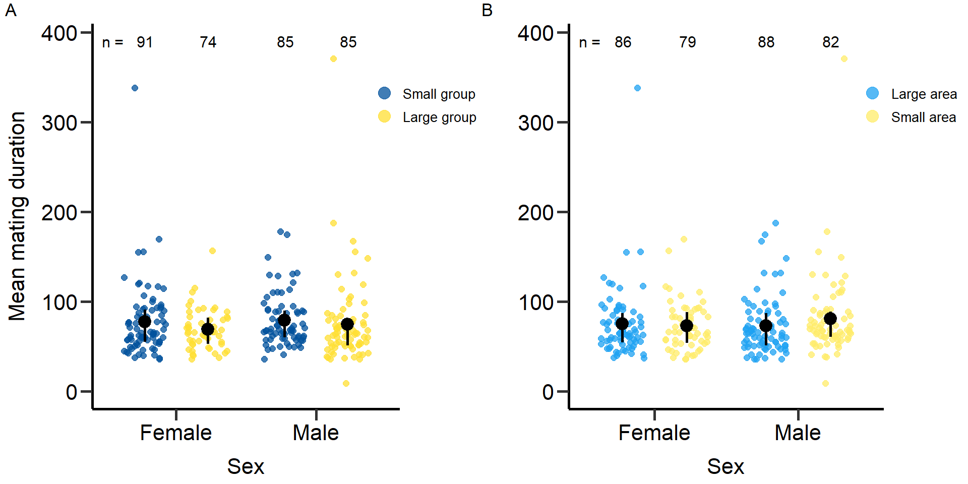 Figure 3: Effects of group size (A) and area treatment (B) on the Mating
duration (in seconds) of female and male focals. Black bars indicate
means and quartile borders.
Figure 3: Effects of group size (A) and area treatment (B) on the Mating
duration (in seconds) of female and male focals. Black bars indicate
means and quartile borders.
Statistical models: Mating duration (Gaussian GLM)
Effect of group size on mating duration in females.
# Statistical models: Mating duration (Gaussian GLM)
# Sex: Female
# Treatment: Group size
mod3.1=glm(f_MatingDuration_av~Gr_size,data=DB_data,family = gaussian)
summary(mod3.1)
Call:
glm(formula = f_MatingDuration_av ~ Gr_size, family = gaussian,
    data = DB_data)

Deviance Residuals:
   Min      1Q  Median      3Q     Max
-41.63  -20.35   -6.36   13.62  260.37

Coefficients:
            Estimate Std. Error t value Pr(>|t|)
(Intercept)   77.626      3.963  19.589   <2e-16 ***
Gr_sizeLG     -8.203      6.266  -1.309    0.193
---
Signif. codes:  0 '***' 0.001 '**' 0.01 '*' 0.05 '.' 0.1 ' ' 1

(Dispersion parameter for gaussian family taken to be 1224.805)

    Null deviance: 158874  on 129  degrees of freedom
Residual deviance: 156775  on 128  degrees of freedom
  (148 Beobachtungen als fehlend gelöscht)
AIC: 1297.3

Number of Fisher Scoring iterations: 2
Effect of group size on mating duration in males.
# Sex: Male
# Treatment: Group size
mod3.2=glm(m_MatingDuration_av~Gr_size,data=DB_data,family = gaussian)
summary(mod3.2)
Call:
glm(formula = m_MatingDuration_av ~ Gr_size, family = gaussian,
    data = DB_data)

Deviance Residuals:
    Min       1Q   Median       3Q      Max
-65.622  -21.472  -10.327    9.798  296.048

Coefficients:
            Estimate Std. Error t value Pr(>|t|)
(Intercept)   79.202      4.594  17.240   <2e-16 ***
Gr_sizeLG     -4.250      6.453  -0.659    0.511
---
Signif. codes:  0 '***' 0.001 '**' 0.01 '*' 0.05 '.' 0.1 ' ' 1

(Dispersion parameter for gaussian family taken to be 1540.677)

    Null deviance: 225607  on 147  degrees of freedom
Residual deviance: 224939  on 146  degrees of freedom
  (130 Beobachtungen als fehlend gelöscht)
AIC: 1510.3

Number of Fisher Scoring iterations: 2
Effect of area on mating duration in females.
# Sex: Female
# Treatment: Area
mod3.3=glm(f_MatingDuration_av~Area,data=DB_data,family = gaussian)
summary(mod3.3)
Call:
glm(formula = f_MatingDuration_av ~ Area, family = gaussian,
    data = DB_data)

Deviance Residuals:
    Min       1Q   Median       3Q      Max
-38.502  -19.592   -7.618   14.121  262.498

Coefficients:
            Estimate Std. Error t value Pr(>|t|)
(Intercept)   75.502      4.178  18.070   <2e-16 ***
AreaSmall     -2.549      6.202  -0.411    0.682
---
Signif. codes:  0 '***' 0.001 '**' 0.01 '*' 0.05 '.' 0.1 ' ' 1

(Dispersion parameter for gaussian family taken to be 1239.57)

    Null deviance: 158874  on 129  degrees of freedom
Residual deviance: 158665  on 128  degrees of freedom
  (148 Beobachtungen als fehlend gelöscht)
AIC: 1298.8

Number of Fisher Scoring iterations: 2
Effect of area on mating duration in males.
# Sex: Male
# Treatment: Area
mod3.4=glm(m_MatingDuration_av~Area,data=DB_data,family = gaussian)
summary(mod3.4)
Call:
glm(formula = m_MatingDuration_av ~ Area, family = gaussian,
    data = DB_data)

Deviance Residuals:
    Min       1Q   Median       3Q      Max
-71.872  -21.242  -10.322    8.445  289.798

Coefficients:
            Estimate Std. Error t value Pr(>|t|)
(Intercept)   73.112      4.485  16.302   <2e-16 ***
AreaSmall      8.090      6.430   1.258     0.21
---
Signif. codes:  0 '***' 0.001 '**' 0.01 '*' 0.05 '.' 0.1 ' ' 1

(Dispersion parameter for gaussian family taken to be 1528.679)

    Null deviance: 225607  on 147  degrees of freedom
Residual deviance: 223187  on 146  degrees of freedom
  (130 Beobachtungen als fehlend gelöscht)
AIC: 1509.2

Number of Fisher Scoring iterations: 2
Mating encounters
# Figure: Mating encounters (mating number + mating attempts)
# Treatment: Group size
p4<-ggplot(DB_data, aes(x=Sex, y=as.numeric(Total_Encounters),fill=Gr_size, col=Gr_size)) +
geom_point(position=position_jitterdodge(jitter.width=0.6,jitter.height = 0,dodge.width=0.9),shape=19, alpha=0.75, size = 2)+
stat_summary(fun.min = function(z) { quantile(z,0.25) },
fun.max = function(z) { quantile(z,0.75) },
fun = mean,position=position_dodge(.9), size = 0.9,col='black',show.legend = F)+
scale_color_manual(values=c(colorESEB[1],colorESEB[2]),name = "Treatment", labels = c('Small group','Large group'))+
scale_fill_manual(values=c(colorESEB[1],colorESEB[2]),name = "Treatment", labels = c('Small group','Large group'))+
xlab('Sex')+ylab("Mating encounters")+ggtitle('')+ theme(plot.title = element_text(hjust = 0.5))+
scale_x_discrete(labels = c('Female','Male'),drop=FALSE)+ ylim(0,33)+labs(tag = "A")+
annotate("text",label='n =',x=0.55,y=33,size=4)+
annotate("text",label='91',x=0.78,y=33,size=4)+
annotate("text",label='74',x=1.23,y=33,size=4)+
annotate("text",label='85',x=1.78,y=33,size=4)+
annotate("text",label='85',x=2.23,y=33,size=4)+
theme(panel.border = element_blank(),
plot.margin = margin(0,2.2,0.15,0.2,"cm"),
plot.title = element_text(hjust = 0.5),
panel.background = element_blank(),
legend.key=element_blank(),
panel.grid.major = element_blank(),
panel.grid.minor = element_blank(),
legend.position = c(1.08, 0.8),
plot.tag.position=c(0.01,0.98),
legend.title = element_blank(),
legend.text = element_text(colour="black", size=10),
axis.line.x = element_line(colour = "black", size = 1),
axis.line.y = element_line(colour = "black", size = 1),
axis.text.x = element_text(face="plain", color="black", size=16, angle=0),
axis.text.y = element_text(face="plain", color="black", size=16, angle=0),
axis.title.x = element_text(size=16,face="plain", margin = margin(r=0,10,0,0)),
axis.title.y = element_text(size=16,face="plain", margin = margin(r=10,0,0,0)),
axis.ticks = element_line(size = 1),
axis.ticks.length = unit(.3, "cm"))+
guides(colour = guide_legend(override.aes = list(size=4)))
# Treatment: Area
p4.2<-ggplot(DB_data, aes(x=Sex, y=as.numeric(Total_Encounters),fill=Area, col=Area)) +
geom_point(position=position_jitterdodge(jitter.width=0.6,jitter.height = 0,dodge.width=0.9),shape=19, alpha=0.75, size = 2)+
stat_summary(fun.min = function(z) { quantile(z,0.25) },
fun.max = function(z) { quantile(z,0.75) },
fun = mean,position=position_dodge(.9), size = 0.9,col='black',show.legend = F)+
scale_color_manual(values=c(colorESEB2[1],colorESEB2[2]),name = "Treatment", labels = c('Large area','Small area'))+
scale_fill_manual(values=c(colorESEB2[1],colorESEB2[2]),name = "Treatment", labels = c('Large area','Small area'))+
xlab('Sex')+ylab("")+ggtitle('')+ theme(plot.title = element_text(hjust = 0.5))+
scale_x_discrete(labels = c('Female','Male'),drop=FALSE)+ ylim(0,33)+labs(tag = "B")+
annotate("text",label='n =',x=0.55,y=33,size=4)+
annotate("text",label='86',x=0.78,y=33,size=4)+
annotate("text",label='79',x=1.23,y=33,size=4)+
annotate("text",label='88',x=1.78,y=33,size=4)+
annotate("text",label='82',x=2.23,y=33,size=4)+
theme(panel.border = element_blank(),
plot.margin = margin(0,2.2,0.15,0,"cm"),
plot.title = element_text(hjust = 0.5),
panel.background = element_blank(),
legend.key=element_blank(),
panel.grid.major = element_blank(),
panel.grid.minor = element_blank(),
legend.position = c(1.08, 0.8),
plot.tag.position=c(0.01,0.98),
legend.title = element_blank(),
legend.text = element_text(colour="black", size=10),
axis.line.x = element_line(colour = "black", size = 1),
axis.line.y = element_line(colour = "black", size = 1),
axis.text.x = element_text(face="plain", color="black", size=16, angle=0),
axis.text.y = element_text(face="plain", color="black", size=16, angle=0),
axis.title.x = element_text(size=16,face="plain", margin = margin(r=0,10,0,0)),
axis.title.y = element_text(size=16,face="plain", margin = margin(r=10,0,0,0)),
axis.ticks = element_line(size = 1),
axis.ticks.length = unit(.3, "cm"))+
guides(colour = guide_legend(override.aes = list(size=4)))
plot4<-grid.arrange(grobs = list(p4,p4.2), nrow = 1,ncol=2, widths=c(2.3, 2.3))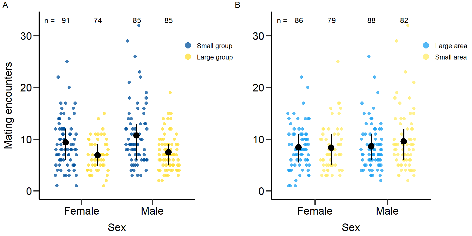 Figure 4: Effects of group size (A) and area treatment (B) on the number
of mating encounters (mating number + mating attempts) of female and
male focals. Black bars indicate means and quartile borders.
Figure 4: Effects of group size (A) and area treatment (B) on the number
of mating encounters (mating number + mating attempts) of female and
male focals. Black bars indicate means and quartile borders.
Statistical models: Mating encounters (Gaussian GLM)
Effect of group size on mating encounters in females.
# Statistical models: Mating encounters (Gaussian GLM)
# Sex: Female
# Treatment: Group size
mod4.1=glm(f_Total_Encounters~Gr_size,data=DB_data,family = gaussian)
summary(mod4.1)
Call:
glm(formula = f_Total_Encounters ~ Gr_size, family = gaussian,
    data = DB_data)

Deviance Residuals:
    Min       1Q   Median       3Q      Max
-8.3718  -2.9038  -0.9038   2.6282  15.6282

Coefficients:
            Estimate Std. Error t value Pr(>|t|)
(Intercept)   9.3718     0.4727  19.827  < 2e-16 ***
Gr_sizeLG    -2.4679     0.7474  -3.302  0.00124 **
---
Signif. codes:  0 '***' 0.001 '**' 0.01 '*' 0.05 '.' 0.1 ' ' 1

(Dispersion parameter for gaussian family taken to be 17.42763)

    Null deviance: 2420.8  on 129  degrees of freedom
Residual deviance: 2230.7  on 128  degrees of freedom
  (148 Beobachtungen als fehlend gelöscht)
AIC: 744.46

Number of Fisher Scoring iterations: 2
Effect of group size on mating encounters in males.
# Sex: Male
# Treatment: Group size
mod4.2=glm(m_Total_Encounters~Gr_size,data=DB_data,family = gaussian)
summary(mod4.2)
Call:
glm(formula = m_Total_Encounters ~ Gr_size, family = gaussian,
    data = DB_data)

Deviance Residuals:
   Min      1Q  Median      3Q     Max
-7.726  -3.453  -0.726   1.728  21.274

Coefficients:
            Estimate Std. Error t value Pr(>|t|)
(Intercept)  10.7260     0.5699  18.822  < 2e-16 ***
Gr_sizeLG    -3.2727     0.8005  -4.088 7.15e-05 ***
---
Signif. codes:  0 '***' 0.001 '**' 0.01 '*' 0.05 '.' 0.1 ' ' 1

(Dispersion parameter for gaussian family taken to be 23.70621)

    Null deviance: 3857.3  on 147  degrees of freedom
Residual deviance: 3461.1  on 146  degrees of freedom
  (130 Beobachtungen als fehlend gelöscht)
AIC: 892.52

Number of Fisher Scoring iterations: 2
Effect of area on mating encounters in females.
# Sex: Female
# Treatment: Area
mod4.3=glm(f_Total_Encounters~Area,data=DB_data,family = gaussian)
summary(mod4.3)
Call:
glm(formula = f_Total_Encounters ~ Area, family = gaussian, data = DB_data)

Deviance Residuals:
    Min       1Q   Median       3Q      Max
-7.4366  -3.3220  -0.4366   2.5634  16.6780

Coefficients:
            Estimate Std. Error t value Pr(>|t|)
(Intercept)   8.4366     0.5161   16.35   <2e-16 ***
AreaSmall    -0.1146     0.7660   -0.15    0.881
---
Signif. codes:  0 '***' 0.001 '**' 0.01 '*' 0.05 '.' 0.1 ' ' 1

(Dispersion parameter for gaussian family taken to be 18.90895)

    Null deviance: 2420.8  on 129  degrees of freedom
Residual deviance: 2420.3  on 128  degrees of freedom
  (148 Beobachtungen als fehlend gelöscht)
AIC: 755.06

Number of Fisher Scoring iterations: 2
Effect of area on mating encounters in males.
# Sex: Male
# Treatment: Area
mod4.4=glm(m_Total_Encounters~Area,data=DB_data,family = gaussian)
summary(mod4.4)
Call:
glm(formula = m_Total_Encounters ~ Area, family = gaussian, data = DB_data)

Deviance Residuals:
   Min      1Q  Median      3Q     Max
-7.556  -3.556  -1.080   2.395  22.444

Coefficients:
            Estimate Std. Error t value Pr(>|t|)
(Intercept)   8.6053     0.5870  14.659   <2e-16 ***
AreaSmall     0.9503     0.8417   1.129    0.261
---
Signif. codes:  0 '***' 0.001 '**' 0.01 '*' 0.05 '.' 0.1 ' ' 1

(Dispersion parameter for gaussian family taken to be 26.19134)

    Null deviance: 3857.3  on 147  degrees of freedom
Residual deviance: 3823.9  on 146  degrees of freedom
  (130 Beobachtungen als fehlend gelöscht)
AIC: 907.28

Number of Fisher Scoring iterations: 2
Proportion of successful matings
# Figure: Proportion of successful matings (mating number/mating number + mating attempts)
# Treatment: Group size
p5<-ggplot(DB_data, aes(x=Sex, y=as.numeric(Prop_MS),fill=Gr_size, col=Gr_size)) +
geom_point(position=position_jitterdodge(jitter.width=0.6,jitter.height = 0,dodge.width=0.9),shape=19, alpha=0.75, size = 2)+
stat_summary(fun.min = function(z) { quantile(z,0.25) },
fun.max = function(z) { quantile(z,0.75) },
fun = mean,position=position_dodge(.9), size = 0.9,col='black',show.legend = F)+
scale_color_manual(values=c(colorESEB[1],colorESEB[2]),name = "Treatment", labels = c('Small group','Large group'))+
scale_fill_manual(values=c(colorESEB[1],colorESEB[2]),name = "Treatment", labels = c('Small group','Large group'))+
xlab('Sex')+ylab("Proportion successful matings")+ggtitle('')+ theme(plot.title = element_text(hjust = 0.5))+
scale_x_discrete(labels = c('Female','Male'),drop=FALSE)+ ylim(0,1.1)+labs(tag = "A")+
annotate("text",label='n =',x=0.55,y=1.1,size=4)+
annotate("text",label='91',x=0.78,y=1.1,size=4)+
annotate("text",label='74',x=1.23,y=1.1,size=4)+
annotate("text",label='85',x=1.78,y=1.1,size=4)+
annotate("text",label='85',x=2.23,y=1.1,size=4)+
theme(panel.border = element_blank(),
plot.margin = margin(0.15,2.2,0,0.2,"cm"),
plot.title = element_text(hjust = 0.5),
panel.background = element_blank(),
legend.key=element_blank(),
panel.grid.major = element_blank(),
panel.grid.minor = element_blank(),
legend.position = c(1.08, 0.8),
plot.tag.position=c(0.01,0.98),
legend.title = element_blank(),
legend.text = element_text(colour="black", size=10),
axis.line.x = element_line(colour = "black", size = 1),
axis.line.y = element_line(colour = "black", size = 1),
axis.text.x = element_text(face="plain", color="black", size=16, angle=0),
axis.text.y = element_text(face="plain", color="black", size=16, angle=0),
axis.title.x = element_text(size=16,face="plain", margin = margin(r=0,10,0,0)),
axis.title.y = element_text(size=16,face="plain", margin = margin(r=10,0,0,0)),
axis.ticks = element_line(size = 1),
axis.ticks.length = unit(.3, "cm"))+
guides(colour = guide_legend(override.aes = list(size=4)))
# Treatment: Area
p5.2<-ggplot(DB_data, aes(x=Sex, y=as.numeric(Prop_MS),fill=Area, col=Area)) +
geom_point(position=position_jitterdodge(jitter.width=0.6,jitter.height = 0,dodge.width=0.9),shape=19, alpha=0.75, size = 2)+
stat_summary(fun.min = function(z) { quantile(z,0.25) },
fun.max = function(z) { quantile(z,0.75) },
fun = mean,position=position_dodge(.9), size = 0.9,col='black',show.legend = F)+
scale_color_manual(values=c(colorESEB2[1],colorESEB2[2]),name = "Treatment", labels = c('Large area','Small area'))+
scale_fill_manual(values=c(colorESEB2[1],colorESEB2[2]),name = "Treatment", labels = c('Large area','Small area'))+
xlab('Sex')+ylab("")+ggtitle('')+ theme(plot.title = element_text(hjust = 0.5))+
scale_x_discrete(labels = c('Female','Male'),drop=FALSE)+ ylim(0,1.1)+labs(tag = "B")+
annotate("text",label='n =',x=0.55,y=1.1,size=4)+
annotate("text",label='86',x=0.78,y=1.1,size=4)+
annotate("text",label='79',x=1.23,y=1.1,size=4)+
annotate("text",label='88',x=1.78,y=1.1,size=4)+
annotate("text",label='82',x=2.23,y=1.1,size=4)+
theme(panel.border = element_blank(),
plot.margin = margin(0.15,2.2,0,0,"cm"),
plot.title = element_text(hjust = 0.5),
panel.background = element_blank(),
legend.key=element_blank(),
panel.grid.major = element_blank(),
panel.grid.minor = element_blank(),
legend.position = c(1.08, 0.8),
plot.tag.position=c(0.01,0.98),
legend.title = element_blank(),
legend.text = element_text(colour="black", size=10),
axis.line.x = element_line(colour = "black", size = 1),
axis.line.y = element_line(colour = "black", size = 1),
axis.text.x = element_text(face="plain", color="black", size=16, angle=0),
axis.text.y = element_text(face="plain", color="black", size=16, angle=0),
axis.title.x = element_text(size=16,face="plain", margin = margin(r=0,10,0,0)),
axis.title.y = element_text(size=16,face="plain", margin = margin(r=10,0,0,0)),
axis.ticks = element_line(size = 1),
axis.ticks.length = unit(.3, "cm"))+
guides(colour = guide_legend(override.aes = list(size=4)))
plot5<-grid.arrange(grobs = list(p5,p5.2), nrow = 1,ncol=2, widths=c(2.3, 2.3))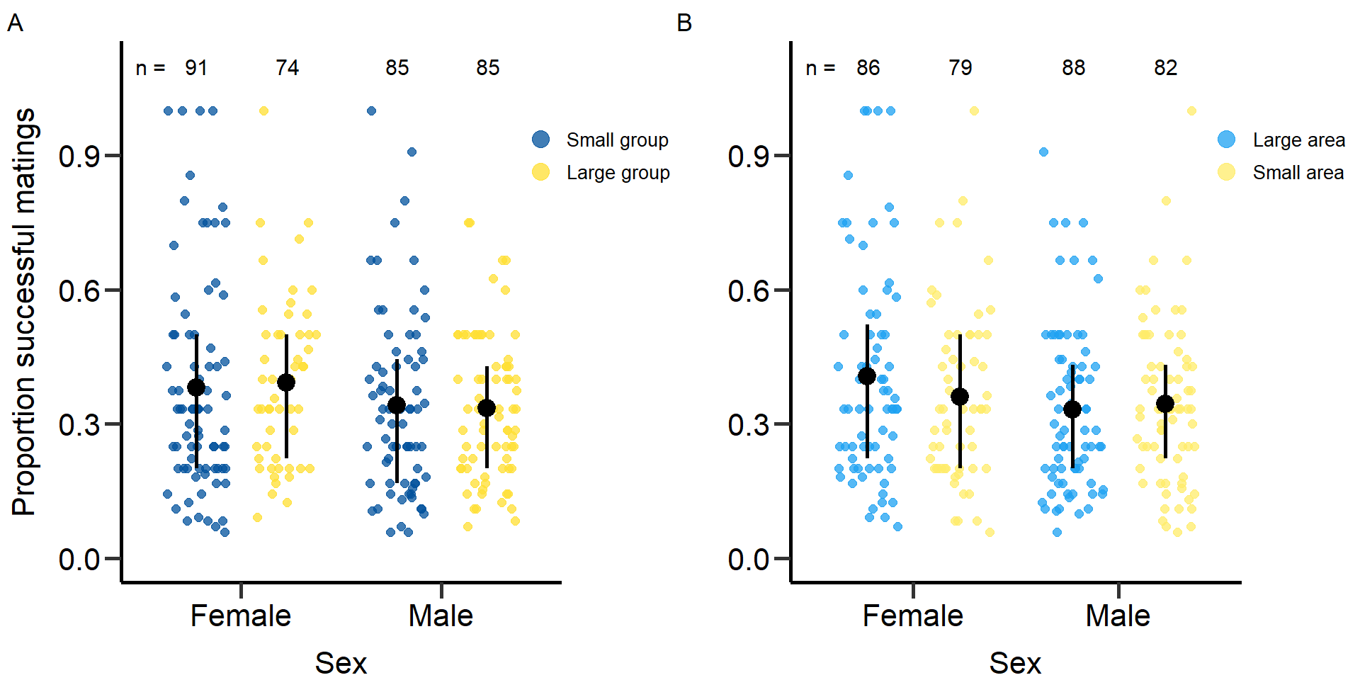 Figure 5: Effects of group size (A) and area treatment (B) on the
proportion of successful matings (mating number/mating number + mating
attempts) of female and male focals. Black bars indicate means and
quartile borders.
Figure 5: Effects of group size (A) and area treatment (B) on the
proportion of successful matings (mating number/mating number + mating
attempts) of female and male focals. Black bars indicate means and
quartile borders.
Statistical models: Proportion of successful matings
(quasi-binomial GLM)
Effect of group size on proportion of
successful matings in females.
# Statistical models: Proportion of successful matings (quasi-binomial GLM)
# Sex: Female
# Treatment: Group size
mod5.1=glm(cbind(f_TotMatings,f_Attempts_number)~Gr_size,data=DB_data,family = quasibinomial)
summary(mod5.1)
Call:
glm(formula = cbind(f_TotMatings, f_Attempts_number) ~ Gr_size,
    family = quasibinomial, data = DB_data)

Deviance Residuals:
    Min       1Q   Median       3Q      Max
-2.8166  -0.8025  -0.0549   0.7731   3.4012

Coefficients:
            Estimate Std. Error t value Pr(>|t|)
(Intercept)  -0.6544     0.0926  -7.067 9.09e-11 ***
Gr_sizeLG     0.1003     0.1598   0.627    0.531
---
Signif. codes:  0 '***' 0.001 '**' 0.01 '*' 0.05 '.' 0.1 ' ' 1

(Dispersion parameter for quasibinomial family taken to be 1.410505)

    Null deviance: 190.01  on 129  degrees of freedom
Residual deviance: 189.45  on 128  degrees of freedom
  (148 Beobachtungen als fehlend gelöscht)
AIC: NA

Number of Fisher Scoring iterations: 4
Effect of group size on proportion of successful matings in
males.
# Sex: Male
# Treatment: Group size
mod5.2=glm(cbind(m_TotMatings,m_Attempts_number)~Gr_size,data=DB_data,family = quasibinomial)
summary(mod5.2)
Call:
glm(formula = cbind(m_TotMatings, m_Attempts_number) ~ Gr_size,
    family = quasibinomial, data = DB_data)

Deviance Residuals:
    Min       1Q   Median       3Q      Max
-2.4940  -0.6358   0.1065   0.7179   4.2524

Coefficients:
            Estimate Std. Error t value Pr(>|t|)
(Intercept) -0.84669    0.08881  -9.533   <2e-16 ***
Gr_sizeLG    0.06083    0.13667   0.445    0.657
---
Signif. codes:  0 '***' 0.001 '**' 0.01 '*' 0.05 '.' 0.1 ' ' 1

(Dispersion parameter for quasibinomial family taken to be 1.297307)

    Null deviance: 194.77  on 147  degrees of freedom
Residual deviance: 194.51  on 146  degrees of freedom
  (130 Beobachtungen als fehlend gelöscht)
AIC: NA

Number of Fisher Scoring iterations: 4
Effect of area on proportion of successful matings in
females.
# Sex: Female
# Treatment: Area
mod5.3=glm(cbind(f_TotMatings,f_Attempts_number)~Area,data=DB_data,family = quasibinomial)
summary(mod5.3)
Call:
glm(formula = cbind(f_TotMatings, f_Attempts_number) ~ Area,
    family = quasibinomial, data = DB_data)

Deviance Residuals:
    Min       1Q   Median       3Q      Max
-2.6934  -0.8646  -0.0321   0.8745   3.1859

Coefficients:
            Estimate Std. Error t value Pr(>|t|)
(Intercept) -0.53673    0.09988  -5.374 3.53e-07 ***
AreaSmall   -0.19021    0.15125  -1.258    0.211
---
Signif. codes:  0 '***' 0.001 '**' 0.01 '*' 0.05 '.' 0.1 ' ' 1

(Dispersion parameter for quasibinomial family taken to be 1.391415)

    Null deviance: 190.01  on 129  degrees of freedom
Residual deviance: 187.80  on 128  degrees of freedom
  (148 Beobachtungen als fehlend gelöscht)
AIC: NA

Number of Fisher Scoring iterations: 4
Effect of area on proportion of successful matings in males.
# Sex: Male
# Treatment: Area
mod5.4=glm(cbind(m_TotMatings,m_Attempts_number)~Area,data=DB_data,family = quasibinomial)
summary(mod5.4)
Call:
glm(formula = cbind(m_TotMatings, m_Attempts_number) ~ Area,
    family = quasibinomial, data = DB_data)

Deviance Residuals:
    Min       1Q   Median       3Q      Max
-2.5859  -0.6372   0.1125   0.7222   4.1648

Coefficients:
            Estimate Std. Error t value Pr(>|t|)
(Intercept) -0.79113    0.09600  -8.241 8.97e-14 ***
AreaSmall   -0.05894    0.13483  -0.437    0.663
---
Signif. codes:  0 '***' 0.001 '**' 0.01 '*' 0.05 '.' 0.1 ' ' 1

(Dispersion parameter for quasibinomial family taken to be 1.293625)

    Null deviance: 194.77  on 147  degrees of freedom
Residual deviance: 194.52  on 146  degrees of freedom
  (130 Beobachtungen als fehlend gelöscht)
AIC: NA

Number of Fisher Scoring iterations: 4
Reproductive success
Secondly, we tested the effect that the treatments (group size and area) had on the reproductive success of focal beetles.
# Figure: Reproductive success
# Treatment: Group size
p6<-ggplot(DB_data_clean, aes(x=Sex, y=as.numeric(Total_N_MTP1),fill=Gr_size, col=Gr_size)) +
geom_point(position=position_jitterdodge(jitter.width=0.6,jitter.height = 0,dodge.width=0.9),shape=19, alpha=0.75, size = 2)+
stat_summary(fun.min = function(z) { quantile(z,0.25) },
fun.max = function(z) { quantile(z,0.75) },
fun = mean,position=position_dodge(.9), size = 0.9,col='black',show.legend = F)+
scale_color_manual(values=c(colorESEB[1],colorESEB[2]),name = "Treatment", labels = c('Small group','Large group'))+
scale_fill_manual(values=c(colorESEB[1],colorESEB[2]),name = "Treatment", labels = c('Small group','Large group'))+
xlab('Sex')+ylab("Number of offspring")+ggtitle('')+ theme(plot.title = element_text(hjust = 0.5))+
scale_x_discrete(labels = c('Female','Male'),drop=FALSE)+ ylim(0,320)+labs(tag = "A")+
annotate("text",label='n =',x=0.55,y=320,size=4)+
annotate("text",label='59',x=0.78,y=320,size=4)+
annotate("text",label='48',x=1.23,y=320,size=4)+
annotate("text",label='51',x=1.78,y=320,size=4)+
annotate("text",label='59',x=2.23,y=320,size=4)+
theme(panel.border = element_blank(),
plot.margin = margin(0,2.2,0,0.2,"cm"),
plot.title = element_text(hjust = 0.5),
panel.background = element_blank(),
legend.key=element_blank(),
panel.grid.major = element_blank(),
panel.grid.minor = element_blank(),
legend.position = c(1.1, 0.8),
plot.tag.position=c(0.01,0.98),
legend.title = element_blank(),
legend.text = element_text(colour="black", size=10),
axis.line.x = element_line(colour = "black", size = 1),
axis.line.y = element_line(colour = "black", size = 1),
axis.text.x = element_text(face="plain", color="black", size=16, angle=0),
axis.text.y = element_text(face="plain", color="black", size=16, angle=0),
axis.title.x = element_text(size=16,face="plain", margin = margin(r=0,10,0,0)),
axis.title.y = element_text(size=16,face="plain", margin = margin(r=10,0,0,0)),
axis.ticks = element_line(size = 1),
axis.ticks.length = unit(.3, "cm"))+
guides(colour = guide_legend(override.aes = list(size=4)))
# Treatment: Area
p6.2<-ggplot(DB_data_clean, aes(x=Sex, y=as.numeric(Total_N_MTP1),fill=Area, col=Area)) +
geom_point(position=position_jitterdodge(jitter.width=0.6,jitter.height = 0,dodge.width=0.9),shape=19, alpha=0.75, size = 2)+
stat_summary(fun.min = function(z) { quantile(z,0.25) },
fun.max = function(z) { quantile(z,0.75) },
fun = mean,position=position_dodge(.9), size = 0.9,col='black',show.legend = F)+
scale_color_manual(values=c(colorESEB2[1],colorESEB2[2]),name = "Treatment", labels = c('Large area','Small area'))+
scale_fill_manual(values=c(colorESEB2[1],colorESEB2[2]),name = "Treatment", labels = c('Large area','Small area'))+
xlab('Sex')+ylab("")+ggtitle('')+ theme(plot.title = element_text(hjust = 0.5))+
scale_x_discrete(labels = c('Female','Male'),drop=FALSE)+ ylim(0,320)+labs(tag = "B")+
annotate("text",label='n =',x=0.55,y=320,size=4)+
annotate("text",label='56',x=0.78,y=320,size=4)+
annotate("text",label='51',x=1.23,y=320,size=4)+
annotate("text",label='57',x=1.78,y=320,size=4)+
annotate("text",label='53',x=2.23,y=320,size=4)+
theme(panel.border = element_blank(),
plot.margin = margin(0,2.2,0,0,"cm"),
plot.title = element_text(hjust = 0.5),
panel.background = element_blank(),
legend.key=element_blank(),
panel.grid.major = element_blank(),
panel.grid.minor = element_blank(),
legend.position = c(1.1, 0.8),
plot.tag.position=c(0.01,0.98),
legend.title = element_blank(),
legend.text = element_text(colour="black", size=10),
axis.line.x = element_line(colour = "black", size = 1),
axis.line.y = element_line(colour = "black", size = 1),
axis.text.x = element_text(face="plain", color="black", size=16, angle=0),
axis.text.y = element_text(face="plain", color="black", size=16, angle=0),
axis.title.x = element_text(size=16,face="plain", margin = margin(r=0,10,0,0)),
axis.title.y = element_text(size=16,face="plain", margin = margin(r=10,0,0,0)),
axis.ticks = element_line(size = 1),
axis.ticks.length = unit(.3, "cm"))+guides(colour = guide_legend(override.aes = list(size=4)))
grid.arrange(grobs = list(p6,p6.2), nrow = 1,ncol=2, widths=c(2.3, 2.3))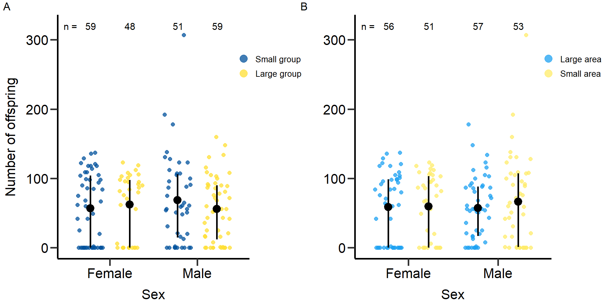 Figure 6: Effects of group size (A) and area treatment (B) on the
reproductive success of female and male focals. Black bars indicate
means and quartile borders.
Figure 6: Effects of group size (A) and area treatment (B) on the
reproductive success of female and male focals. Black bars indicate
means and quartile borders.
Statistical models: Reproductive success (quasi-Poisson
GLM)
Effect of group size on reproductive success in
females.
# Statistical models: Reproductive success (quasi-Poisson GLM)
# Sex: Female
# Treatment: Group size
mod6.1=glm(f_RS~Gr_size,data=DB_data_clean,family = quasipoisson)
summary(mod6.1)
Call:
glm(formula = f_RS ~ Gr_size, family = quasipoisson, data = DB_data_clean)

Deviance Residuals:
    Min       1Q   Median       3Q      Max
-11.143  -10.664    1.433    4.942    8.982

Coefficients:
            Estimate Std. Error t value Pr(>|t|)
(Intercept)  4.04054    0.12007  33.650   <2e-16 ***
Gr_sizeLG    0.08801    0.18288   0.481    0.632
---
Signif. codes:  0 '***' 0.001 '**' 0.01 '*' 0.05 '.' 0.1 ' ' 1

(Dispersion parameter for quasipoisson family taken to be 40.16879)

    Null deviance: 4614.9  on 82  degrees of freedom
Residual deviance: 4605.7  on 81  degrees of freedom
  (94 Beobachtungen als fehlend gelöscht)
AIC: NA

Number of Fisher Scoring iterations: 5
Effect of group size on reproductive success in males.
# Sex: Male
# Treatment: Group size
mod6.2=glm(m_RS~Gr_size,data=DB_data_clean,family = quasipoisson)
summary(mod6.2)
Call:
glm(formula = m_RS ~ Gr_size, family = quasipoisson, data = DB_data_clean)

Deviance Residuals:
     Min        1Q    Median        3Q       Max
-11.7196   -7.9610   -0.7465    4.1631   21.0427

Coefficients:
            Estimate Std. Error t value Pr(>|t|)
(Intercept)    4.229      0.127  33.308   <2e-16 ***
Gr_sizeLG     -0.203      0.181  -1.121    0.265
---
Signif. codes:  0 '***' 0.001 '**' 0.01 '*' 0.05 '.' 0.1 ' ' 1

(Dispersion parameter for quasipoisson family taken to be 47.61251)

    Null deviance: 5078.4  on 93  degrees of freedom
Residual deviance: 5018.5  on 92  degrees of freedom
  (83 Beobachtungen als fehlend gelöscht)
AIC: NA

Number of Fisher Scoring iterations: 5
Effect of area on reproductive success in females.
# Sex: Female
# Treatment: Area
mod6.3=glm(f_RS~Area,data=DB_data_clean,family = quasipoisson)
summary(mod6.3)
Call:
glm(formula = f_RS ~ Area, family = quasipoisson, data = DB_data_clean)

Deviance Residuals:
    Min       1Q   Median       3Q      Max
-10.920  -10.817    1.581    4.922    8.727

Coefficients:
            Estimate Std. Error t value Pr(>|t|)
(Intercept)  4.06903    0.12200  33.354   <2e-16 ***
AreaSmall    0.01899    0.18177   0.104    0.917
---
Signif. codes:  0 '***' 0.001 '**' 0.01 '*' 0.05 '.' 0.1 ' ' 1

(Dispersion parameter for quasipoisson family taken to be 40.05135)

    Null deviance: 4614.9  on 82  degrees of freedom
Residual deviance: 4614.5  on 81  degrees of freedom
  (94 Beobachtungen als fehlend gelöscht)
AIC: NA

Number of Fisher Scoring iterations: 5
Effect of area on reproductive success in males.
# Sex: Male
# Treatment: Area
mod6.4=glm(m_RS~Area,data=DB_data_clean,family = quasipoisson)
summary(mod6.4)
Call:
glm(formula = m_RS ~ Area, family = quasipoisson, data = DB_data_clean)

Deviance Residuals:
    Min       1Q   Median       3Q      Max
-11.536   -7.447   -0.200    3.954   21.400

Coefficients:
            Estimate Std. Error t value Pr(>|t|)
(Intercept)   4.0520     0.1306  31.034   <2e-16 ***
AreaSmall     0.1457     0.1819   0.801    0.425
---
Signif. codes:  0 '***' 0.001 '**' 0.01 '*' 0.05 '.' 0.1 ' ' 1

(Dispersion parameter for quasipoisson family taken to be 48.03915)

    Null deviance: 5078.4  on 93  degrees of freedom
Residual deviance: 5047.5  on 92  degrees of freedom
  (83 Beobachtungen als fehlend gelöscht)
AIC: NA

Number of Fisher Scoring iterations: 5
Metrics of sexual selection
In this part of our analysis we estimated standardized metrics of
(sexual) selection.
Metrics:
- Opportunity for selection
- Opportunity for sexual selection
- Bateman gradient
- Jones
index
We used bootstrapping (10.000 bootstrap replicates) to
obtain 95% confidence intervals and permutation tests (10.000
permutations) to statistically compare treatments and sexes.
# Opportunity for selection
#Area
DB_data_clean_Large_area_Male_rel_propRS <-as.data.table(DB_data_clean_Large_area$rel_m_RS)
c <- function(d, i){
  d2 <- d[i,]
  return(var(d2[,1], na.rm=TRUE))
}
I_Large_area_Male_bootvar <- boot(DB_data_clean_Large_area_Male_rel_propRS, c, R=10000)

DB_data_clean_Large_area_Female_rel_propRS <-as.data.table(DB_data_clean_Large_area$rel_f_RS)

I_Large_area_Female_bootvar <- boot(DB_data_clean_Large_area_Female_rel_propRS, c, R=10000)

DB_data_clean_Small_area_Male_rel_propRS <-as.data.table(DB_data_clean_Small_area$rel_m_RS)

I_Small_area_Male_bootvar <- boot(DB_data_clean_Small_area_Male_rel_propRS, c, R=10000)

DB_data_clean_Small_area_Female_rel_propRS <-as.data.table(DB_data_clean_Small_area$rel_f_RS)

I_Small_area_Female_bootvar <- boot(DB_data_clean_Small_area_Female_rel_propRS, c, R=10000)

#Population size
DB_data_clean_Large_pop_Male_rel_propRS <-as.data.table(DB_data_clean_Large_pop$rel_m_RS)

I_Large_pop_Male_bootvar <- boot(DB_data_clean_Large_pop_Male_rel_propRS, c, R=10000)

DB_data_clean_Large_pop_Female_rel_propRS <-as.data.table(DB_data_clean_Large_pop$rel_f_RS)

I_Large_pop_Female_bootvar <- boot(DB_data_clean_Large_pop_Female_rel_propRS, c, R=10000)

DB_data_clean_Small_pop_Male_rel_propRS <-as.data.table(DB_data_clean_Small_pop$rel_m_RS)

I_Small_pop_Male_bootvar <- boot(DB_data_clean_Small_pop_Male_rel_propRS, c, R=10000)

DB_data_clean_Small_pop_Female_rel_propRS <-as.data.table(DB_data_clean_Small_pop$rel_f_RS)

I_Small_pop_Female_bootvar <- boot(DB_data_clean_Small_pop_Female_rel_propRS, c, R=10000)
rm("c")

# Opportunity for sexual selection
#Area
DB_data_clean_Large_area_Male_relMS <-as.data.table(DB_data_clean_Large_area$rel_m_cMS)
c <- function(d, i){
  d2 <- d[i,]
  return(var(d2[,1], na.rm=TRUE))
}
Is_Large_area_Male_bootvar <- boot(DB_data_clean_Large_area_Male_relMS, c, R=10000)

DB_data_clean_Large_area_Female_relMS <-as.data.table(DB_data_clean_Large_area$rel_f_cMS)

Is_Large_area_Female_bootvar <- boot(DB_data_clean_Large_area_Female_relMS, c, R=10000)

DB_data_clean_Small_area_Male_relMS <-as.data.table(DB_data_clean_Small_area$rel_m_cMS)

Is_Small_area_Male_bootvar <- boot(DB_data_clean_Small_area_Male_relMS, c, R=10000)

DB_data_clean_Small_area_Female_relMS <-as.data.table(DB_data_clean_Small_area$rel_f_cMS)

Is_Small_area_Female_bootvar <- boot(DB_data_clean_Small_area_Female_relMS, c, R=10000)

#Population size
DB_data_clean_Large_pop_Male_relMS <-as.data.table(DB_data_clean_Large_pop$rel_m_cMS)

Is_Large_pop_Male_bootvar <- boot(DB_data_clean_Large_pop_Male_relMS, c, R=10000)

DB_data_clean_Large_pop_Female_relMS <-as.data.table(DB_data_clean_Large_pop$rel_f_cMS)

Is_Large_pop_Female_bootvar <- boot(DB_data_clean_Large_pop_Female_relMS, c, R=10000)

DB_data_clean_Small_pop_Male_relMS <-as.data.table(DB_data_clean_Small_pop$rel_m_cMS)

Is_Small_pop_Male_bootvar <- boot(DB_data_clean_Small_pop_Male_relMS, c, R=10000)

DB_data_clean_Small_pop_Female_relMS <-as.data.table(DB_data_clean_Small_pop$rel_f_cMS)

Is_Small_pop_Female_bootvar <- boot(DB_data_clean_Small_pop_Female_relMS, c, R=10000)
rm("c")

# Bateman Gradient
#Area
DB_data_clean_Large_area_Male_B <-as.data.table(cbind(DB_data_clean_Large_area$rel_m_RS,DB_data_clean_Large_area$rel_m_cMS))

c <- function(d, i){
  d2 <- d[i,]
  return(lm(V1 ~V2,data=d2)$coefficients[2])
}
B_Large_area_Male_bootvar <- boot(DB_data_clean_Large_area_Male_B, c, R=10000)

DB_data_clean_Small_area_Male_B <-as.data.table(cbind(DB_data_clean_Small_area$rel_m_RS,DB_data_clean_Small_area$rel_m_cMS))

B_Small_area_Male_bootvar <- boot(DB_data_clean_Small_area_Male_B, c, R=10000)

DB_data_clean_Large_area_Female_B <-as.data.table(cbind(DB_data_clean_Large_area$rel_f_RS,DB_data_clean_Large_area$rel_f_cMS))

B_Large_area_Female_bootvar <- boot(DB_data_clean_Large_area_Female_B, c, R=10000)

DB_data_clean_Small_area_Female_B <-as.data.table(cbind(DB_data_clean_Small_area$rel_f_RS,DB_data_clean_Small_area$rel_f_cMS))

B_Small_area_Female_bootvar <- boot(DB_data_clean_Small_area_Female_B, c, R=10000)

#Population size
DB_data_clean_Large_pop_Male_B <-as.data.table(cbind(DB_data_clean_Large_pop$rel_m_RS,DB_data_clean_Large_pop$rel_m_cMS))

B_Large_pop_Male_bootvar <- boot(DB_data_clean_Large_pop_Male_B, c, R=10000)

DB_data_clean_Small_pop_Male_B <-as.data.table(cbind(DB_data_clean_Small_pop$rel_m_RS,DB_data_clean_Small_pop$rel_m_cMS))

B_Small_pop_Male_bootvar <- boot(DB_data_clean_Small_pop_Male_B, c, R=10000)

DB_data_clean_Large_pop_Female_B <-as.data.table(cbind(DB_data_clean_Large_pop$rel_f_RS,DB_data_clean_Large_pop$rel_f_cMS))

B_Large_pop_Female_bootvar <- boot(DB_data_clean_Large_pop_Female_B, c, R=10000)

DB_data_clean_Small_pop_Female_B <-as.data.table(cbind(DB_data_clean_Small_pop$rel_f_RS,DB_data_clean_Small_pop$rel_f_cMS))

B_Small_pop_Female_bootvar <- boot(DB_data_clean_Small_pop_Female_B, c, R=10000)
rm("c")

#Jones index
#Area

c <- function(d, i){
  d2 <- d[i,]
  return(lm(d2$V1 ~d2$V2)$coefficients[2]*sqrt(var(d2$V2, na.rm=TRUE)))
}

S_Large_area_Male_bootvar <- boot(DB_data_clean_Large_area_Male_B, c, R=10000)

S_Small_area_Male_bootvar <- boot(DB_data_clean_Small_area_Male_B, c, R=10000)

S_Large_area_Female_bootvar <- boot(DB_data_clean_Large_area_Female_B, c, R=10000)

S_Small_area_Female_bootvar <- boot(DB_data_clean_Small_area_Female_B, c, R=10000)

#Population size

S_Large_pop_Male_bootvar <- boot(DB_data_clean_Large_pop_Male_B, c, R=10000)

S_Small_pop_Male_bootvar <- boot(DB_data_clean_Small_pop_Male_B, c, R=10000)

S_Large_pop_Female_bootvar <- boot(DB_data_clean_Large_pop_Female_B, c, R=10000)

S_Small_pop_Female_bootvar <- boot(DB_data_clean_Small_pop_Female_B, c, R=10000)
rm("c")

#Make data table
PhenVarBoot_Table_Male_Small_pop_I <- as.data.frame(cbind("Male", "Small_pop", "Opportunity for selection", as.numeric(mean(I_Small_pop_Male_bootvar$t)), quantile(I_Small_pop_Male_bootvar$t,.025, names = FALSE), quantile(I_Small_pop_Male_bootvar$t,.975, names = FALSE)))
PhenVarBoot_Table_Male_Large_pop_I <- as.data.frame(cbind("Male", "Large_pop", "Opportunity for selection", mean(I_Large_pop_Male_bootvar$t), quantile(I_Large_pop_Male_bootvar$t,.025, names = FALSE), quantile(I_Large_pop_Male_bootvar$t,.975, names = FALSE)))
PhenVarBoot_Table_Male_Large_area_I <- as.data.frame(cbind("Male", "Large_area", "Opportunity for selection", mean(I_Large_area_Male_bootvar$t), quantile(I_Large_area_Male_bootvar$t,.025, names = FALSE), quantile(I_Large_area_Male_bootvar$t,.975, names = FALSE)))
PhenVarBoot_Table_Male_Small_area_I <- as.data.frame(cbind("Male", "Small_area", "Opportunity for selection", mean(I_Small_area_Male_bootvar$t), quantile(I_Small_area_Male_bootvar$t,.025, names = FALSE), quantile(I_Small_area_Male_bootvar$t,.975, names = FALSE)))
PhenVarBoot_Table_Male_Small_pop_Is <- as.data.frame(cbind("Male", "Small_pop", "Opportunity for sexual selection", mean(Is_Small_pop_Male_bootvar$t), quantile(Is_Small_pop_Male_bootvar$t,.025, names = FALSE), quantile(Is_Small_pop_Male_bootvar$t,.975, names = FALSE)))
PhenVarBoot_Table_Male_Large_pop_Is <- as.data.frame(cbind("Male", "Large_pop", "Opportunity for sexual selection", mean(Is_Large_pop_Male_bootvar$t), quantile(Is_Large_pop_Male_bootvar$t,.025, names = FALSE), quantile(Is_Large_pop_Male_bootvar$t,.975, names = FALSE)))
PhenVarBoot_Table_Male_Large_area_Is <- as.data.frame(cbind("Male", "Large_area", "Opportunity for sexual selection", mean(Is_Large_area_Male_bootvar$t), quantile(Is_Large_area_Male_bootvar$t,.025, names = FALSE), quantile(Is_Large_area_Male_bootvar$t,.975, names = FALSE)))
PhenVarBoot_Table_Male_Small_area_Is <- as.data.frame(cbind("Male", "Small_area", "Opportunity for sexual selection", mean(Is_Small_area_Male_bootvar$t), quantile(Is_Small_area_Male_bootvar$t,.025, names = FALSE), quantile(Is_Small_area_Male_bootvar$t,.975, names = FALSE)))
PhenVarBoot_Table_Male_Small_pop_B <- as.data.frame(cbind("Male", "Small_pop", "Bateman gradient", mean(B_Small_pop_Male_bootvar$t), quantile(B_Small_pop_Male_bootvar$t,.025, names = FALSE), quantile(B_Small_pop_Male_bootvar$t,.975, names = FALSE)))
PhenVarBoot_Table_Male_Large_pop_B <- as.data.frame(cbind("Male", "Large_pop", "Bateman gradient", mean(B_Large_pop_Male_bootvar$t), quantile(B_Large_pop_Male_bootvar$t,.025, names = FALSE), quantile(B_Large_pop_Male_bootvar$t,.975, names = FALSE)))
PhenVarBoot_Table_Male_Large_area_B <- as.data.frame(cbind("Male", "Large_area", "Bateman gradient", mean(B_Large_area_Male_bootvar$t), quantile(B_Large_area_Male_bootvar$t,.025, names = FALSE), quantile(B_Large_area_Male_bootvar$t,.975, names = FALSE)))
PhenVarBoot_Table_Male_Small_area_B <- as.data.frame(cbind("Male", "Small_area", "Bateman gradient", mean(B_Small_area_Male_bootvar$t), quantile(B_Small_area_Male_bootvar$t,.025, names = FALSE), quantile(B_Small_area_Male_bootvar$t,.975, names = FALSE)))
PhenVarBoot_Table_Male_Small_pop_S <- as.data.frame(cbind("Male", "Small_pop", "Maximum standardized sexual selection differential", mean(S_Small_pop_Male_bootvar$t,na.rm = T), quantile(S_Small_pop_Male_bootvar$t,.025, names = FALSE,na.rm = T), quantile(S_Small_pop_Male_bootvar$t,.975, names = FALSE,na.rm = T)))
PhenVarBoot_Table_Male_Large_pop_S <- as.data.frame(cbind("Male", "Large_pop", "Maximum standardized sexual selection differential", mean(S_Large_pop_Male_bootvar$t,na.rm = T), quantile(S_Large_pop_Male_bootvar$t,.025, names = FALSE,na.rm = T), quantile(S_Large_pop_Male_bootvar$t,.975, names = FALSE,na.rm = T)))
PhenVarBoot_Table_Male_Large_area_S <- as.data.frame(cbind("Male", "Large_area", "Maximum standardized sexual selection differential", mean(S_Large_area_Male_bootvar$t,na.rm = T), quantile(S_Large_area_Male_bootvar$t,.025, names = FALSE,na.rm = T), quantile(S_Large_area_Male_bootvar$t,.975, names = FALSE,na.rm = T)))
PhenVarBoot_Table_Male_Small_area_S <- as.data.frame(cbind("Male", "Small_area", "Maximum standardized sexual selection differential", mean(S_Small_area_Male_bootvar$t,na.rm = T), quantile(S_Small_area_Male_bootvar$t,.025, names = FALSE,na.rm = T), quantile(S_Small_area_Male_bootvar$t,.975, names = FALSE,na.rm = T)))

PhenVarBoot_Table_Female_Small_pop_I <- as.data.frame(cbind("Female", "Small_pop", "Opportunity for selection", mean(I_Small_pop_Female_bootvar$t), quantile(I_Small_pop_Female_bootvar$t,.025, names = FALSE), quantile(I_Small_pop_Female_bootvar$t,.975, names = FALSE)))
PhenVarBoot_Table_Female_Large_pop_I <- as.data.frame(cbind("Female", "Large_pop", "Opportunity for selection", mean(I_Large_pop_Female_bootvar$t), quantile(I_Large_pop_Female_bootvar$t,.025, names = FALSE), quantile(I_Large_pop_Female_bootvar$t,.975, names = FALSE)))
PhenVarBoot_Table_Female_Large_area_I <- as.data.frame(cbind("Female", "Large_area", "Opportunity for selection", mean(I_Large_area_Female_bootvar$t), quantile(I_Large_area_Female_bootvar$t,.025, names = FALSE), quantile(I_Large_area_Female_bootvar$t,.975, names = FALSE)))
PhenVarBoot_Table_Female_Small_area_I <- as.data.frame(cbind("Female", "Small_area", "Opportunity for selection", mean(I_Small_area_Female_bootvar$t), quantile(I_Small_area_Female_bootvar$t,.025, names = FALSE), quantile(I_Small_area_Female_bootvar$t,.975, names = FALSE)))
PhenVarBoot_Table_Female_Small_pop_Is <- as.data.frame(cbind("Female", "Small_pop", "Opportunity for sexual selection", mean(Is_Small_pop_Female_bootvar$t), quantile(Is_Small_pop_Female_bootvar$t,.025, names = FALSE), quantile(Is_Small_pop_Female_bootvar$t,.975, names = FALSE)))
PhenVarBoot_Table_Female_Large_pop_Is <- as.data.frame(cbind("Female", "Large_pop", "Opportunity for sexual selection", mean(Is_Large_pop_Female_bootvar$t), quantile(Is_Large_pop_Female_bootvar$t,.025, names = FALSE), quantile(Is_Large_pop_Female_bootvar$t,.975, names = FALSE)))
PhenVarBoot_Table_Female_Large_area_Is <- as.data.frame(cbind("Female", "Large_area", "Opportunity for sexual selection", mean(Is_Large_area_Female_bootvar$t), quantile(Is_Large_area_Female_bootvar$t,.025, names = FALSE), quantile(Is_Large_area_Female_bootvar$t,.975, names = FALSE)))
PhenVarBoot_Table_Female_Small_area_Is <- as.data.frame(cbind("Female", "Small_area", "Opportunity for sexual selection", mean(Is_Small_area_Female_bootvar$t), quantile(Is_Small_area_Female_bootvar$t,.025, names = FALSE), quantile(Is_Small_area_Female_bootvar$t,.975, names = FALSE)))
PhenVarBoot_Table_Female_Small_pop_B <- as.data.frame(cbind("Female", "Small_pop", "Bateman gradient", mean(B_Small_pop_Female_bootvar$t), quantile(B_Small_pop_Female_bootvar$t,.025, names = FALSE), quantile(B_Small_pop_Female_bootvar$t,.975, names = FALSE)))
PhenVarBoot_Table_Female_Large_pop_B <- as.data.frame(cbind("Female", "Large_pop", "Bateman gradient", mean(B_Large_pop_Female_bootvar$t), quantile(B_Large_pop_Female_bootvar$t,.025, names = FALSE), quantile(B_Large_pop_Female_bootvar$t,.975, names = FALSE)))
PhenVarBoot_Table_Female_Large_area_B <- as.data.frame(cbind("Female", "Large_area", "Bateman gradient", mean(B_Large_area_Female_bootvar$t), quantile(B_Large_area_Female_bootvar$t,.025, names = FALSE), quantile(B_Large_area_Female_bootvar$t,.975, names = FALSE)))
PhenVarBoot_Table_Female_Small_area_B <- as.data.frame(cbind("Female", "Small_area", "Bateman gradient", mean(B_Small_area_Female_bootvar$t), quantile(B_Small_area_Female_bootvar$t,.025, names = FALSE), quantile(B_Small_area_Female_bootvar$t,.975, names = FALSE)))
PhenVarBoot_Table_Female_Small_pop_S <- as.data.frame(cbind("Female", "Small_pop", "Maximum standardized sexual selection differential", mean(S_Small_pop_Female_bootvar$t,na.rm = T), quantile(S_Small_pop_Female_bootvar$t,.025, names = FALSE,na.rm = T), quantile(S_Small_pop_Female_bootvar$t,.975, names = FALSE,na.rm = T)))
PhenVarBoot_Table_Female_Large_pop_S <- as.data.frame(cbind("Female", "Large_pop", "Maximum standardized sexual selection differential", mean(S_Large_pop_Female_bootvar$t,na.rm = T), quantile(S_Large_pop_Female_bootvar$t,.025, names = FALSE,na.rm = T), quantile(S_Large_pop_Female_bootvar$t,.975, names = FALSE,na.rm = T)))
PhenVarBoot_Table_Female_Large_area_S <- as.data.frame(cbind("Female", "Large_area", "Maximum standardized sexual selection differential", mean(S_Large_area_Female_bootvar$t,na.rm = T), quantile(S_Large_area_Female_bootvar$t,.025, names = FALSE,na.rm = T), quantile(S_Large_area_Female_bootvar$t,.975, names = FALSE,na.rm = T)))
PhenVarBoot_Table_Female_Small_area_S <- as.data.frame(cbind("Female", "Small_area", "Maximum standardized sexual selection differential", mean(S_Small_area_Female_bootvar$t,na.rm = T), quantile(S_Small_area_Female_bootvar$t,.025, names = FALSE,na.rm = T), quantile(S_Small_area_Female_bootvar$t,.975, names = FALSE,na.rm = T)))


Table_BatemanMetrics <- as.data.frame(as.matrix(rbind(PhenVarBoot_Table_Male_Small_pop_I,PhenVarBoot_Table_Male_Large_pop_I,PhenVarBoot_Table_Male_Large_area_I,PhenVarBoot_Table_Male_Small_area_I,
                                                      PhenVarBoot_Table_Male_Small_pop_Is,PhenVarBoot_Table_Male_Large_pop_Is,PhenVarBoot_Table_Male_Large_area_Is,PhenVarBoot_Table_Male_Small_area_Is,
                                                      PhenVarBoot_Table_Male_Small_pop_B,PhenVarBoot_Table_Male_Large_pop_B,PhenVarBoot_Table_Male_Large_area_B,PhenVarBoot_Table_Male_Small_area_B,
                                                      PhenVarBoot_Table_Male_Small_pop_S,PhenVarBoot_Table_Male_Large_pop_S,PhenVarBoot_Table_Male_Large_area_S,PhenVarBoot_Table_Male_Small_area_S,
                                                      PhenVarBoot_Table_Female_Small_pop_I,PhenVarBoot_Table_Female_Large_pop_I,PhenVarBoot_Table_Female_Large_area_I,PhenVarBoot_Table_Female_Small_area_I,
                                                      PhenVarBoot_Table_Female_Small_pop_Is,PhenVarBoot_Table_Female_Large_pop_Is,PhenVarBoot_Table_Female_Large_area_Is,PhenVarBoot_Table_Female_Small_area_Is,
                                                      PhenVarBoot_Table_Female_Small_pop_B,PhenVarBoot_Table_Female_Large_pop_B,PhenVarBoot_Table_Female_Large_area_B,PhenVarBoot_Table_Female_Small_area_B,
                                                      PhenVarBoot_Table_Female_Small_pop_S,PhenVarBoot_Table_Female_Large_pop_S,PhenVarBoot_Table_Female_Large_area_S,PhenVarBoot_Table_Female_Small_area_S)),digits=3)

is.table(Table_BatemanMetrics)
colnames(Table_BatemanMetrics)[1] <- "Sex"
colnames(Table_BatemanMetrics)[2] <- "Treatment"
colnames(Table_BatemanMetrics)[3] <- "Variable"
colnames(Table_BatemanMetrics)[4] <- "Variance"
colnames(Table_BatemanMetrics)[5] <- "l95.CI"
colnames(Table_BatemanMetrics)[6] <- "u95.CI"
Table_BatemanMetrics[,4]=as.numeric(Table_BatemanMetrics[,4])
Table_BatemanMetrics[,5]=as.numeric(Table_BatemanMetrics[,5])
Table_BatemanMetrics[,6]=as.numeric(Table_BatemanMetrics[,6])
#Bootstrap treatment comparisons
#I
#Area
#Males
Treat_diff_Male_area_I=c(I_Large_area_Male_bootvar$t)-c(I_Small_area_Male_bootvar$t)
t_Treat_diff_Male_area_I=mean(Treat_diff_Male_area_I,na.rm=TRUE)
t_Treat_diff_Male_area_I_lower=quantile(Treat_diff_Male_area_I,.025,na.rm=TRUE)
t_Treat_diff_Male_area_I_upper=quantile(Treat_diff_Male_area_I,.975,na.rm=TRUE)
#Permutation test to calculate p value
comb_data=c(DB_data_clean_Large_area$rel_m_RS,DB_data_clean_Small_area$rel_m_RS)
diff.observed = var(na.omit((DB_data_clean_Large_area$rel_m_RS))) - var(na.omit((DB_data_clean_Small_area$rel_m_RS)))
diff.observed
number_of_permutations = 100000
diff.random = NULL
for (i in 1 : number_of_permutations) {
# Sample from the combined dataset
a.random = sample (na.omit(comb_data), length(c(DB_data_clean_Large_area$rel_m_RS)), TRUE)
b.random = sample (na.omit(comb_data), length(c(DB_data_clean_Small_area$rel_m_RS)), TRUE)
# Null (permuated) difference
diff.random[i] = var(na.omit(b.random)) - var(na.omit(a.random))
}
# P-value is the fraction of how many times the permuted difference is
# equal or more extreme than the observed difference
t_Treat_diff_Male_area_I_p = sum(abs(diff.random) >= as.numeric(abs(diff.observed)))/ number_of_permutations
#Females
Treat_diff_Female_area_I=c(I_Large_area_Female_bootvar$t)-c(I_Small_area_Female_bootvar$t)
t_Treat_diff_Female_area_I=mean(Treat_diff_Female_area_I,na.rm=TRUE)
t_Treat_diff_Female_area_I_lower=quantile(Treat_diff_Female_area_I,.025,na.rm=TRUE)
t_Treat_diff_Female_area_I_upper=quantile(Treat_diff_Female_area_I,.975,na.rm=TRUE)
#Permutation test to calculate p value
comb_data=c(DB_data_clean_Large_area$rel_f_RS,DB_data_clean_Small_area$rel_f_RS)
diff.observed = var(na.omit((DB_data_clean_Large_area$rel_f_RS))) - var(na.omit((DB_data_clean_Small_area$rel_f_RS)))
diff.observed
number_of_permutations = 100000
diff.random = NULL
for (i in 1 : number_of_permutations) {
# Sample from the combined dataset
a.random = sample (na.omit(comb_data), length(c(DB_data_clean_Large_area$rel_f_RS)), TRUE)
b.random = sample (na.omit(comb_data), length(c(DB_data_clean_Small_area$rel_f_RS)), TRUE)
# Null (permuated) difference
diff.random[i] = var(na.omit(b.random)) - var(na.omit(a.random))
}
# P-value is the fraction of how many times the permuted difference is
# equal or more extreme than the observed difference
t_Treat_diff_Female_area_I_p = sum(abs(diff.random) >= as.numeric(abs(diff.observed)))/ number_of_permutations
#Population size ####
#Males
Treat_diff_Male_pop_I=c(I_Small_pop_Male_bootvar$t)-c(I_Large_pop_Male_bootvar$t)
t_Treat_diff_Male_pop_I=mean(Treat_diff_Male_pop_I,na.rm=TRUE)
t_Treat_diff_Male_pop_I_lower=quantile(Treat_diff_Male_pop_I,.025,na.rm=TRUE)
t_Treat_diff_Male_pop_I_upper=quantile(Treat_diff_Male_pop_I,.975,na.rm=TRUE)
#Permutation test to calculate p value
comb_data=c(DB_data_clean_Small_pop$rel_m_RS,DB_data_clean_Large_pop$rel_m_RS)
diff.observed = var(na.omit((DB_data_clean_Small_pop$rel_m_RS))) - var(na.omit((DB_data_clean_Large_pop$rel_m_RS)))
diff.observed
number_of_permutations = 100000
diff.random = NULL
for (i in 1 : number_of_permutations) {
# Sample from the combined dataset
a.random = sample (na.omit(comb_data), length(c(DB_data_clean_Small_pop$rel_m_RS)), TRUE)
b.random = sample (na.omit(comb_data), length(c(DB_data_clean_Large_pop$rel_m_RS)), TRUE)
# Null (permuated) difference
diff.random[i] = var(na.omit(b.random)) - var(na.omit(a.random))
}
# P-value is the fraction of how many times the permuted difference is
# equal or more extreme than the observed difference
t_Treat_diff_Male_pop_I_p = sum(abs(diff.random) >= as.numeric(abs(diff.observed)))/ number_of_permutations
#Females
Treat_diff_Female_pop_I=c(I_Small_pop_Female_bootvar$t)-c(I_Large_pop_Female_bootvar$t)
t_Treat_diff_Female_pop_I=mean(Treat_diff_Female_pop_I,na.rm=TRUE)
t_Treat_diff_Female_pop_I_lower=quantile(Treat_diff_Female_pop_I,.025,na.rm=TRUE)
t_Treat_diff_Female_pop_I_upper=quantile(Treat_diff_Female_pop_I,.975,na.rm=TRUE)
#Permutation test to calculate p value
comb_data=c(DB_data_clean_Small_pop$rel_f_RS,DB_data_clean_Large_pop$rel_f_RS)
diff.observed = var(na.omit(c(DB_data_clean_Small_pop$rel_f_RS))) - var(na.omit(c(DB_data_clean_Large_pop$rel_f_RS)))
diff.observed
number_of_permutations = 100000
diff.random = NULL
for (i in 1 : number_of_permutations) {
# Sample from the combined dataset
a.random = sample (na.omit(comb_data), length(c(DB_data_clean_Small_pop$rel_f_RS)), TRUE)
b.random = sample (na.omit(comb_data), length(c(DB_data_clean_Large_pop$rel_f_RS)), TRUE)
# Null (permuated) difference
diff.random[i] = var(na.omit(b.random)) - var(na.omit(a.random))
}
# P-value is the fraction of how many times the permuted difference is
# equal or more extreme than the observed difference
t_Treat_diff_Female_pop_I_p = sum(abs(diff.random) >= as.numeric(abs(diff.observed)))/ number_of_permutations
#Is ####
#Area ####
#Males
Treat_diff_Male_area_Is=c(Is_Large_area_Male_bootvar$t)-c(Is_Small_area_Male_bootvar$t)
t_Treat_diff_Male_area_Is=mean(Treat_diff_Male_area_Is,na.rm=TRUE)
t_Treat_diff_Male_area_Is_lower=quantile(Treat_diff_Male_area_Is,.025,na.rm=TRUE)
t_Treat_diff_Male_area_Is_upper=quantile(Treat_diff_Male_area_Is,.975,na.rm=TRUE)
#Permutation test to calculate p value
comb_data=c(DB_data_clean_Large_area$rel_m_cMS,DB_data_clean_Small_area$rel_m_cMS)
diff.observed = var(na.omit(c(DB_data_clean_Large_area$rel_m_cMS))) - var(na.omit(c(DB_data_clean_Small_area$rel_m_cMS)))
diff.observed
number_of_permutations = 100000
diff.random = NULL
for (i in 1 : number_of_permutations) {
# Sample from the combined dataset
a.random = sample (na.omit(comb_data), length(c(DB_data_clean_Large_area$rel_m_cMS)), TRUE)
b.random = sample (na.omit(comb_data), length(c(DB_data_clean_Small_area$rel_m_cMS)), TRUE)
# Null (permuated) difference
diff.random[i] = var(na.omit(b.random)) - var(na.omit(a.random))
}
# P-value is the fraction of how many times the permuted difference is
# equal or more extreme than the observed difference
t_Treat_diff_Male_area_Is_p = sum(abs(diff.random) >= as.numeric(abs(diff.observed)))/ number_of_permutations
#Females
Treat_diff_Female_area_Is=c(Is_Large_area_Female_bootvar$t)-c(Is_Small_area_Female_bootvar$t)
t_Treat_diff_Female_area_Is=mean(Treat_diff_Female_area_Is,na.rm=TRUE)
t_Treat_diff_Female_area_Is_lower=quantile(Treat_diff_Female_area_Is,.025,na.rm=TRUE)
t_Treat_diff_Female_area_Is_upper=quantile(Treat_diff_Female_area_Is,.975,na.rm=TRUE)
#Permutation test to calculate p value
comb_data=c(DB_data_clean_Large_area$rel_f_cMS,DB_data_clean_Small_area$rel_f_cMS)
diff.observed = var(na.omit(c(DB_data_clean_Large_area$rel_f_cMS))) - var(na.omit(c(DB_data_clean_Small_area$rel_f_cMS)))
diff.observed
number_of_permutations = 100000
diff.random = NULL
for (i in 1 : number_of_permutations) {
# Sample from the combined dataset
a.random = sample (na.omit(comb_data), length(c(DB_data_clean_Large_area$rel_f_cMS)), TRUE)
b.random = sample (na.omit(comb_data), length(c(DB_data_clean_Small_area$rel_f_cMS)), TRUE)
# Null (permuated) difference
diff.random[i] = var(na.omit(b.random)) - var(na.omit(a.random))
}
# P-value is the fraction of how many times the permuted difference is
# equal or more extreme than the observed difference
t_Treat_diff_Female_area_Is_p = sum(abs(diff.random) >= as.numeric(abs(diff.observed)))/ number_of_permutations
#Population size ####
#Males
Treat_diff_Male_pop_Is=c(Is_Small_pop_Male_bootvar$t)-c(Is_Large_pop_Male_bootvar$t)
t_Treat_diff_Male_pop_Is=mean(Treat_diff_Male_pop_Is,na.rm=TRUE)
t_Treat_diff_Male_pop_Is_lower=quantile(Treat_diff_Male_pop_Is,.025,na.rm=TRUE)
t_Treat_diff_Male_pop_Is_upper=quantile(Treat_diff_Male_pop_Is,.975,na.rm=TRUE)
#Permutation test to calculate p value
comb_data=c(DB_data_clean_Small_pop$rel_m_cMS,DB_data_clean_Large_pop$rel_m_cMS)
diff.observed = var(na.omit(DB_data_clean_Small_pop$rel_m_cMS),na.rm = T) - var(na.omit(DB_data_clean_Large_pop$rel_m_cMS))
diff.observed
number_of_permutations = 100000
diff.random = NULL
for (i in 1 : number_of_permutations) {
# Sample from the combined dataset
a.random = sample (na.omit(comb_data), length(DB_data_clean_Small_pop$rel_m_cMS), TRUE)
b.random = sample (na.omit(comb_data), length(DB_data_clean_Large_pop$rel_m_cMS), TRUE)
# Null (permuated) difference
diff.random[i] = var(na.omit(b.random)) - var(na.omit(a.random))
}
# P-value is the fraction of how many times the permuted difference is
# equal or more extreme than the observed difference
t_Treat_diff_Male_pop_Is_p = sum(abs(diff.random) >= as.numeric(abs(diff.observed)))/ number_of_permutations
#Females
Treat_diff_Female_pop_Is=c(Is_Small_pop_Female_bootvar$t)-c(Is_Large_pop_Female_bootvar$t)
t_Treat_diff_Female_pop_Is=mean(Treat_diff_Female_pop_Is,na.rm=TRUE)
t_Treat_diff_Female_pop_Is_lower=quantile(Treat_diff_Female_pop_Is,.025,na.rm=TRUE)
t_Treat_diff_Female_pop_Is_upper=quantile(Treat_diff_Female_pop_Is,.975,na.rm=TRUE)
#Permutation test to calculate p value
comb_data=c(DB_data_clean_Small_pop$rel_f_cMS,DB_data_clean_Large_pop$rel_f_cMS)
diff.observed = var(na.omit(DB_data_clean_Small_pop$rel_f_cMS)) - var(na.omit(DB_data_clean_Large_pop$rel_f_cMS))
diff.observed
number_of_permutations = 100000
diff.random = NULL
for (i in 1 : number_of_permutations) {
# Sample from the combined dataset
a.random = sample (na.omit(comb_data), length(c(DB_data_clean_Small_pop$rel_f_cMS)), TRUE)
b.random = sample (na.omit(comb_data), length(c(DB_data_clean_Large_pop$rel_f_cMS)), TRUE)
# Null (permuated) difference
diff.random[i] = var(na.omit(b.random)) - var(na.omit(a.random))
}
# P-value is the fraction of how many times the permuted difference is
# equal or more extreme than the observed difference
t_Treat_diff_Female_pop_Is_p = sum(abs(diff.random) >= as.numeric(abs(diff.observed)))/ number_of_permutations
#B ####
#Area ####
#Males
Treat_diff_Male_area_B=c(B_Large_area_Male_bootvar$t)-c(B_Small_area_Male_bootvar$t)
t_Treat_diff_Male_area_B=mean(Treat_diff_Male_area_B,na.rm=TRUE)
t_Treat_diff_Male_area_B_lower=quantile(Treat_diff_Male_area_B,.025,na.rm=TRUE)
t_Treat_diff_Male_area_B_upper=quantile(Treat_diff_Male_area_B,.975,na.rm=TRUE)
#Permutation test to calculate p value
comb_data1=c(DB_data_clean_Large_area$rel_m_RS, DB_data_clean_Small_area$rel_m_RS)
comb_data2=c(DB_data_clean_Large_area$rel_m_cMS,DB_data_clean_Small_area$rel_m_cMS)
diff.observed = lm(DB_data_clean_Large_area$rel_m_RS ~DB_data_clean_Large_area$rel_m_cMS)$coefficients[2] - lm(DB_data_clean_Small_area$rel_m_RS ~DB_data_clean_Small_area$rel_m_cMS)$coefficients[2]
diff.observed
number_of_permutations = 100000
diff.random = NULL
for (i in 1 : number_of_permutations) {
# Sample from the combined dataset
a.random = sample (na.omit(comb_data1), length(DB_data_clean_Large_area$rel_m_RS), TRUE)
b.random = sample (na.omit(comb_data1), length(DB_data_clean_Small_area$rel_m_RS), TRUE)
c.random = sample (na.omit(comb_data2), length(DB_data_clean_Large_area$rel_m_cMS), TRUE)
d.random = sample (na.omit(comb_data2), length(DB_data_clean_Small_area$rel_m_cMS), TRUE)
# Null (permuated) difference
diff.random[i] = lm(a.random ~c.random)$coefficients[2] - lm(b.random ~d.random)$coefficients[2]
}
# P-value is the fraction of how many times the permuted difference is
# equal or more extreme than the observed difference
t_Treat_diff_Male_area_B_p = sum(abs(diff.random) >= as.numeric(abs(diff.observed)))/ number_of_permutations
#Females
Treat_diff_Female_area_B=c(B_Large_area_Female_bootvar$t)-c(B_Small_area_Female_bootvar$t)
t_Treat_diff_Female_area_B=mean(Treat_diff_Female_area_B,na.rm=TRUE)
t_Treat_diff_Female_area_B_lower=quantile(Treat_diff_Female_area_B,.025,na.rm=TRUE)
t_Treat_diff_Female_area_B_upper=quantile(Treat_diff_Female_area_B,.975,na.rm=TRUE)
#Permutation test to calculate p value
comb_data1=c(DB_data_clean_Large_area$rel_f_RS, DB_data_clean_Small_area$rel_f_RS)
comb_data2=c(DB_data_clean_Large_area$rel_f_cMS,DB_data_clean_Small_area$rel_f_cMS)
diff.observed = lm(DB_data_clean_Large_area$rel_f_RS ~DB_data_clean_Large_area$rel_f_cMS)$coefficients[2] - lm(DB_data_clean_Small_area$rel_f_RS ~DB_data_clean_Small_area$rel_f_cMS)$coefficients[2]
diff.observed
number_of_permutations = 100000
diff.random = NULL
for (i in 1 : number_of_permutations) {
# Sample from the combined dataset
a.random = sample (na.omit(comb_data1), length(DB_data_clean_Large_area$rel_f_RS), TRUE)
b.random = sample (na.omit(comb_data1), length(DB_data_clean_Small_area$rel_f_RS), TRUE)
c.random = sample (na.omit(comb_data2), length(DB_data_clean_Large_area$rel_f_cMS), TRUE)
d.random = sample (na.omit(comb_data2), length(DB_data_clean_Small_area$rel_f_cMS), TRUE)
# Null (permuated) difference
diff.random[i] = lm(a.random ~c.random)$coefficients[2] - lm(b.random ~d.random)$coefficients[2]
}
# P-value is the fraction of how many times the permuted difference is
# equal or more extreme than the observed difference
t_Treat_diff_Female_area_B_p = sum(abs(diff.random) >= as.numeric(abs(diff.observed)))/ number_of_permutations
#Population size ####
#Males
Treat_diff_Male_pop_B=c(B_Small_pop_Male_bootvar$t)-c(B_Large_pop_Male_bootvar$t)
t_Treat_diff_Male_pop_B=mean(Treat_diff_Male_pop_B,na.rm=TRUE)
t_Treat_diff_Male_pop_B_lower=quantile(Treat_diff_Male_pop_B,.025,na.rm=TRUE)
t_Treat_diff_Male_pop_B_upper=quantile(Treat_diff_Male_pop_B,.975,na.rm=TRUE)
#Permutation test to calculate p value
comb_data1=c(DB_data_clean_Small_pop$rel_m_RS, DB_data_clean_Large_pop$rel_m_RS)
comb_data2=c(DB_data_clean_Small_pop$rel_m_cMS,DB_data_clean_Large_pop$rel_m_cMS)
diff.observed = lm(DB_data_clean_Small_pop$rel_m_RS ~DB_data_clean_Small_pop$rel_m_cMS)$coefficients[2] - lm(DB_data_clean_Large_pop$rel_m_RS ~DB_data_clean_Large_pop$rel_m_cMS)$coefficients[2]
diff.observed
number_of_permutations = 100000
diff.random = NULL
for (i in 1 : number_of_permutations) {
# Sample from the combined dataset
a.random = sample (na.omit(comb_data1), length(DB_data_clean_Small_pop$rel_m_RS), TRUE)
b.random = sample (na.omit(comb_data1), length(DB_data_clean_Large_pop$rel_m_RS), TRUE)
c.random = sample (na.omit(comb_data2), length(DB_data_clean_Small_pop$rel_m_cMS), TRUE)
d.random = sample (na.omit(comb_data2), length(DB_data_clean_Large_pop$rel_m_cMS), TRUE)
# Null (permuated) difference
diff.random[i] = lm(a.random ~c.random)$coefficients[2] - lm(b.random ~d.random)$coefficients[2]
}
# P-value is the fraction of how many times the permuted difference is
# equal or more extreme than the observed difference
t_Treat_diff_Male_pop_B_p = sum(abs(diff.random) >= as.numeric(abs(diff.observed)))/ number_of_permutations
#Females
Treat_diff_Female_pop_B=c(B_Small_pop_Female_bootvar$t)-c(B_Large_pop_Female_bootvar$t)
t_Treat_diff_Female_pop_B=mean(Treat_diff_Female_pop_B,na.rm=TRUE)
t_Treat_diff_Female_pop_B_lower=quantile(Treat_diff_Female_pop_B,.025,na.rm=TRUE)
t_Treat_diff_Female_pop_B_upper=quantile(Treat_diff_Female_pop_B,.975,na.rm=TRUE)
#Permutation test to calculate p value
comb_data1=c(DB_data_clean_Small_pop$rel_f_RS, DB_data_clean_Large_pop$rel_f_RS)
comb_data2=c(DB_data_clean_Small_pop$rel_f_cMS,DB_data_clean_Large_pop$rel_f_cMS)
diff.observed = lm(DB_data_clean_Small_pop$rel_f_RS ~DB_data_clean_Small_pop$rel_f_cMS)$coefficients[2] - lm(DB_data_clean_Large_pop$rel_f_RS ~DB_data_clean_Large_pop$rel_f_cMS)$coefficients[2]
diff.observed
number_of_permutations = 100000
diff.random = NULL
for (i in 1 : number_of_permutations) {
# Sample from the combined dataset
a.random = sample (na.omit(comb_data1), length(DB_data_clean_Small_pop$rel_f_RS), TRUE)
b.random = sample (na.omit(comb_data1), length(DB_data_clean_Large_pop$rel_f_RS), TRUE)
c.random = sample (na.omit(comb_data2), length(DB_data_clean_Small_pop$rel_f_cMS), TRUE)
d.random = sample (na.omit(comb_data2), length(DB_data_clean_Large_pop$rel_f_cMS), TRUE)
# Null (permuated) difference
diff.random[i] = lm(a.random ~c.random)$coefficients[2] - lm(b.random ~d.random)$coefficients[2]
}
# P-value is the fraction of how many times the permuted difference is
# equal or more extreme than the observed difference
t_Treat_diff_Female_pop_B_p = sum(abs(diff.random) >= as.numeric(abs(diff.observed)))/ number_of_permutations
#S ####
#Area ####
#Males
Treat_diff_Male_area_S=c(S_Large_area_Male_bootvar$t)-c(S_Small_area_Male_bootvar$t)
t_Treat_diff_Male_area_S=mean(Treat_diff_Male_area_S,na.rm=TRUE)
t_Treat_diff_Male_area_S_lower=quantile(Treat_diff_Male_area_S,.025,na.rm=TRUE)
t_Treat_diff_Male_area_S_upper=quantile(Treat_diff_Male_area_S,.975,na.rm=TRUE)
#Permutation test to calculate p value
comb_data1=c(DB_data_clean_Large_area$rel_m_cMS, DB_data_clean_Small_area$rel_m_cMS)
comb_data2=c(DB_data_clean_Large_area$rel_m_RS, DB_data_clean_Small_area$rel_m_RS)
diff.observed = lm(DB_data_clean_Large_area$rel_m_RS ~DB_data_clean_Large_area$rel_m_cMS)$coefficients[2]*sqrt(var(DB_data_clean_Large_area$rel_m_cMS, na.rm=TRUE)) - lm(DB_data_clean_Small_area$rel_m_RS ~DB_data_clean_Small_area$rel_m_cMS)$coefficients[2]*sqrt(var(DB_data_clean_Small_area$rel_m_cMS, na.rm=TRUE))
diff.observed
number_of_permutations = 100000
diff.random = NULL
for (i in 1 : number_of_permutations) {
# Sample from the combined dataset
a.random = sample (na.omit(comb_data1), length(DB_data_clean_Large_area$rel_m_cMS), TRUE)
b.random = sample (na.omit(comb_data1), length(DB_data_clean_Small_area$rel_m_cMS), TRUE)
c.random = sample (na.omit(comb_data2), length(DB_data_clean_Large_area$rel_m_RS), TRUE)
d.random = sample (na.omit(comb_data2), length(DB_data_clean_Small_area$rel_m_RS), TRUE)
# Null (permuated) difference
diff.random[i] = lm(c.random ~a.random)$coefficients[2]*sqrt(var(a.random, na.rm=TRUE)) - lm(d.random ~b.random)$coefficients[2]*sqrt(var(b.random, na.rm=TRUE))
}
# P-value is the fraction of how many times the permuted difference is
# equal or more extreme than the observed difference
t_Treat_diff_Male_area_S_p = sum(abs(diff.random) >= as.numeric(abs(diff.observed)))/ number_of_permutations
#Females
Treat_diff_Female_area_S=c(S_Large_area_Female_bootvar$t)-c(S_Small_area_Female_bootvar$t)
t_Treat_diff_Female_area_S=mean(Treat_diff_Female_area_S,na.rm=TRUE)
t_Treat_diff_Female_area_S_lower=quantile(Treat_diff_Female_area_S,.025,na.rm=TRUE)
t_Treat_diff_Female_area_S_upper=quantile(Treat_diff_Female_area_S,.975,na.rm=TRUE)
#Permutation test to calculate p value
comb_data1=c(DB_data_clean_Large_area$rel_f_cMS, DB_data_clean_Small_area$rel_f_cMS)
comb_data2=c(DB_data_clean_Large_area$rel_f_RS, DB_data_clean_Small_area$rel_f_RS)
diff.observed = lm(DB_data_clean_Large_area$rel_f_RS ~DB_data_clean_Large_area$rel_f_cMS)$coefficients[2]*sqrt(var(DB_data_clean_Large_area$rel_f_cMS, na.rm=TRUE)) - lm(DB_data_clean_Small_area$rel_f_RS ~DB_data_clean_Small_area$rel_f_cMS)$coefficients[2]*sqrt(var(DB_data_clean_Small_area$rel_f_cMS, na.rm=TRUE))
diff.observed
number_of_permutations = 100000
diff.random = NULL
for (i in 1 : number_of_permutations) {
# Sample from the combined dataset
a.random = sample (na.omit(comb_data1), length(DB_data_clean_Large_area$rel_f_cMS), TRUE)
b.random = sample (na.omit(comb_data1), length(DB_data_clean_Small_area$rel_f_cMS), TRUE)
c.random = sample (na.omit(comb_data2), length(DB_data_clean_Large_area$rel_f_RS), TRUE)
d.random = sample (na.omit(comb_data2), length(DB_data_clean_Small_area$rel_f_RS), TRUE)
# Null (permuated) difference
diff.random[i] = lm(c.random ~a.random)$coefficients[2]*sqrt(var(a.random, na.rm=TRUE)) - lm(d.random ~b.random)$coefficients[2]*sqrt(var(b.random, na.rm=TRUE))
}
# P-value is the fraction of how many times the permuted difference is
# equal or more extreme than the observed difference
t_Treat_diff_Female_area_S_p = sum(abs(diff.random) >= as.numeric(abs(diff.observed)))/ number_of_permutations
#Population size ####
#Males
Treat_diff_Male_pop_S=c(S_Small_pop_Male_bootvar$t)-c(S_Large_pop_Male_bootvar$t)
t_Treat_diff_Male_pop_S=mean(Treat_diff_Male_pop_S,na.rm=TRUE)
t_Treat_diff_Male_pop_S_lower=quantile(Treat_diff_Male_pop_S,.025,na.rm=TRUE)
t_Treat_diff_Male_pop_S_upper=quantile(Treat_diff_Male_pop_S,.975,na.rm=TRUE)
#Permutation test to calculate p value
comb_data1=c(DB_data_clean_Small_pop$rel_m_cMS, DB_data_clean_Large_pop$rel_m_cMS)
comb_data2=c(DB_data_clean_Small_pop$rel_m_RS, DB_data_clean_Large_pop$rel_m_RS)
diff.observed = lm(DB_data_clean_Small_pop$rel_m_RS ~DB_data_clean_Small_pop$rel_m_cMS)$coefficients[2]*sqrt(var(DB_data_clean_Small_pop$rel_m_cMS, na.rm=TRUE)) - lm(DB_data_clean_Large_pop$rel_m_RS ~DB_data_clean_Large_pop$rel_m_cMS)$coefficients[2]*sqrt(var(DB_data_clean_Large_pop$rel_m_cMS, na.rm=TRUE))
diff.observed
number_of_permutations = 100000
diff.random = NULL
for (i in 1 : number_of_permutations) {
# Sample from the combined dataset
a.random = sample (na.omit(comb_data1), length(DB_data_clean_Small_pop$rel_m_cMS), TRUE)
b.random = sample (na.omit(comb_data1), length(DB_data_clean_Large_pop$rel_m_cMS), TRUE)
c.random = sample (na.omit(comb_data2), length(DB_data_clean_Small_pop$rel_m_RS), TRUE)
d.random = sample (na.omit(comb_data2), length(DB_data_clean_Large_pop$rel_m_RS), TRUE)
# Null (permuated) difference
diff.random[i] = lm(c.random ~a.random)$coefficients[2]*sqrt(var(a.random, na.rm=TRUE)) - lm(d.random ~b.random)$coefficients[2]*sqrt(var(b.random, na.rm=TRUE))
}
# P-value is the fraction of how many times the permuted difference is
# equal or more extreme than the observed difference
t_Treat_diff_Male_pop_S_p = sum(abs(diff.random) >= as.numeric(abs(diff.observed)))/ number_of_permutations
#Females
Treat_diff_Female_pop_S=c(S_Small_pop_Female_bootvar$t)-c(S_Large_pop_Female_bootvar$t)
t_Treat_diff_Female_pop_S=mean(Treat_diff_Female_pop_S,na.rm=TRUE)
t_Treat_diff_Female_pop_S_lower=quantile(Treat_diff_Female_pop_S,.025,na.rm=TRUE)
t_Treat_diff_Female_pop_S_upper=quantile(Treat_diff_Female_pop_S,.975,na.rm=TRUE)
#Permutation test to calculate p value
comb_data1=c(DB_data_clean_Small_pop$rel_f_cMS, DB_data_clean_Large_pop$rel_f_cMS)
comb_data2=c(DB_data_clean_Small_pop$rel_f_RS, DB_data_clean_Large_pop$rel_f_RS)
diff.observed = lm(DB_data_clean_Small_pop$rel_f_RS ~DB_data_clean_Small_pop$rel_f_cMS)$coefficients[2]*sqrt(var(DB_data_clean_Small_pop$rel_f_cMS, na.rm=TRUE)) - lm(DB_data_clean_Large_pop$rel_f_RS ~DB_data_clean_Large_pop$rel_f_cMS)$coefficients[2]*sqrt(var(DB_data_clean_Large_pop$rel_f_cMS, na.rm=TRUE))
diff.observed
number_of_permutations = 100000
diff.random = NULL
for (i in 1 : number_of_permutations) {
# Sample from the combined dataset
a.random = sample (na.omit(comb_data1), length(DB_data_clean_Small_pop$rel_f_cMS), TRUE)
b.random = sample (na.omit(comb_data1), length(DB_data_clean_Large_pop$rel_f_cMS), TRUE)
c.random = sample (na.omit(comb_data2), length(DB_data_clean_Small_pop$rel_f_RS), TRUE)
d.random = sample (na.omit(comb_data2), length(DB_data_clean_Large_pop$rel_f_RS), TRUE)
# Null (permuated) difference
diff.random[i] = lm(c.random ~a.random)$coefficients[2]*sqrt(var(a.random, na.rm=TRUE)) - lm(d.random ~b.random)$coefficients[2]*sqrt(var(b.random, na.rm=TRUE))
}
# P-value is the fraction of how many times the permuted difference is
# equal or more extreme than the observed difference
t_Treat_diff_Female_pop_S_p = sum(abs(diff.random) >= as.numeric(abs(diff.observed)))/ number_of_permutations
#Save data table ####
CompTreat_Table_Male_area_I <- as.data.frame(cbind("Male", "Area", "Opportunity for selection", t_Treat_diff_Male_area_I, t_Treat_diff_Male_area_I_lower, t_Treat_diff_Male_area_I_upper, t_Treat_diff_Male_area_I_p))
names(CompTreat_Table_Male_area_I)=c('V1','V2','V3','V4','V5','V6','V7')
CompTreat_Table_Male_pop_I <- as.data.frame(cbind("Male", "Group size", "Opportunity for selection", t_Treat_diff_Male_pop_I, t_Treat_diff_Male_pop_I_lower, t_Treat_diff_Male_pop_I_upper, t_Treat_diff_Male_pop_I_p))
names(CompTreat_Table_Male_pop_I)=c('V1','V2','V3','V4','V5','V6','V7')
CompTreat_Table_Male_area_Is <- as.data.frame(cbind("Male", "Area", "Opportunity for sexual selection", t_Treat_diff_Male_area_Is, t_Treat_diff_Male_area_Is_lower, t_Treat_diff_Male_area_Is_upper, t_Treat_diff_Male_area_Is_p))
names(CompTreat_Table_Male_area_Is)=c('V1','V2','V3','V4','V5','V6','V7')
CompTreat_Table_Male_pop_Is <- as.data.frame(cbind("Male", "Group size", "Opportunity for sexual selection", t_Treat_diff_Male_pop_Is, t_Treat_diff_Male_pop_Is_lower, t_Treat_diff_Male_pop_Is_upper, t_Treat_diff_Male_pop_Is_p))
names(CompTreat_Table_Male_pop_Is)=c('V1','V2','V3','V4','V5','V6','V7')
CompTreat_Table_Male_area_B <- as.data.frame(cbind("Male", "Area", "Bateman gradient", t_Treat_diff_Male_area_B, t_Treat_diff_Male_area_B_lower, t_Treat_diff_Male_area_B_upper, t_Treat_diff_Male_area_B_p))
names(CompTreat_Table_Male_area_B)=c('V1','V2','V3','V4','V5','V6','V7')
CompTreat_Table_Male_pop_B <- as.data.frame(cbind("Male", "Group size", "Bateman gradient", t_Treat_diff_Male_pop_B, t_Treat_diff_Male_pop_B_lower, t_Treat_diff_Male_pop_B_upper, t_Treat_diff_Male_pop_B_p))
names(CompTreat_Table_Male_pop_B)=c('V1','V2','V3','V4','V5','V6','V7')
CompTreat_Table_Male_area_S <- as.data.frame(cbind("Male", "Area", "Jones index", t_Treat_diff_Male_area_S, t_Treat_diff_Male_area_S_lower, t_Treat_diff_Male_area_S_upper, t_Treat_diff_Male_area_S_p))
names(CompTreat_Table_Male_area_S)=c('V1','V2','V3','V4','V5','V6','V7')
CompTreat_Table_Male_pop_S <- as.data.frame(cbind("Male", "Group size", "Jones index", t_Treat_diff_Male_pop_S, t_Treat_diff_Male_pop_S_lower, t_Treat_diff_Male_pop_S_upper, t_Treat_diff_Male_pop_S_p))
names(CompTreat_Table_Male_pop_S)=c('V1','V2','V3','V4','V5','V6','V7')
CompTreat_Table_Female_area_I <- as.data.frame(cbind("Female", "Area", "Opportunity for selection", t_Treat_diff_Female_area_I, t_Treat_diff_Female_area_I_lower, t_Treat_diff_Female_area_I_upper, t_Treat_diff_Female_area_I_p))
names(CompTreat_Table_Female_area_I)=c('V1','V2','V3','V4','V5','V6','V7')
CompTreat_Table_Female_pop_I <- as.data.frame(cbind("Female", "Group size", "Opportunity for selection", t_Treat_diff_Female_pop_I, t_Treat_diff_Female_pop_I_lower, t_Treat_diff_Female_pop_I_upper, t_Treat_diff_Female_pop_I_p))
names(CompTreat_Table_Female_pop_I)=c('V1','V2','V3','V4','V5','V6','V7')
CompTreat_Table_Female_area_Is <- as.data.frame(cbind("Female", "Area", "Opportunity for sexual selection", t_Treat_diff_Female_area_Is, t_Treat_diff_Female_area_Is_lower, t_Treat_diff_Female_area_Is_upper, t_Treat_diff_Female_area_Is_p))
names(CompTreat_Table_Female_area_Is)=c('V1','V2','V3','V4','V5','V6','V7')
CompTreat_Table_Female_pop_Is <- as.data.frame(cbind("Female", "Group size", "Opportunity for sexual selection", t_Treat_diff_Female_pop_Is, t_Treat_diff_Female_pop_Is_lower, t_Treat_diff_Female_pop_Is_upper, t_Treat_diff_Female_pop_Is_p))
names(CompTreat_Table_Female_pop_Is)=c('V1','V2','V3','V4','V5','V6','V7')
CompTreat_Table_Female_area_B <- as.data.frame(cbind("Female", "Area", "Bateman gradient", t_Treat_diff_Female_area_B, t_Treat_diff_Female_area_B_lower, t_Treat_diff_Female_area_B_upper, t_Treat_diff_Female_area_B_p))
names(CompTreat_Table_Female_area_B)=c('V1','V2','V3','V4','V5','V6','V7')
CompTreat_Table_Female_pop_B <- as.data.frame(cbind("Female", "Group size", "Bateman gradient", t_Treat_diff_Female_pop_B, t_Treat_diff_Female_pop_B_lower, t_Treat_diff_Female_pop_B_upper, t_Treat_diff_Female_pop_B_p))
names(CompTreat_Table_Female_pop_B)=c('V1','V2','V3','V4','V5','V6','V7')
CompTreat_Table_Female_area_S <- as.data.frame(cbind("Female", "Area", "Jones index", t_Treat_diff_Female_area_S, t_Treat_diff_Female_area_S_lower, t_Treat_diff_Female_area_S_upper, t_Treat_diff_Female_area_S_p))
names(CompTreat_Table_Female_area_S)=c('V1','V2','V3','V4','V5','V6','V7')
CompTreat_Table_Female_pop_S <- as.data.frame(cbind("Female", "Group size", "Jones index", t_Treat_diff_Female_pop_S, t_Treat_diff_Female_pop_S_lower, t_Treat_diff_Female_pop_S_upper, t_Treat_diff_Female_pop_S_p))
names(CompTreat_Table_Female_pop_S)=c('V1','V2','V3','V4','V5','V6','V7')
Table_BatemanMetrics_TreatComp <- as.data.frame(as.matrix(rbind(CompTreat_Table_Male_area_I,CompTreat_Table_Male_area_Is,
CompTreat_Table_Male_area_B,CompTreat_Table_Male_area_S,
CompTreat_Table_Male_pop_I,CompTreat_Table_Male_pop_Is,
CompTreat_Table_Male_pop_B,CompTreat_Table_Male_pop_S,
CompTreat_Table_Female_area_I,CompTreat_Table_Female_area_Is,
CompTreat_Table_Female_area_B,CompTreat_Table_Female_area_S,
CompTreat_Table_Female_pop_I,CompTreat_Table_Female_pop_Is,
CompTreat_Table_Female_pop_B,CompTreat_Table_Female_pop_S
)))
Table_BatemanMetrics_TreatComp[,4]=as.numeric(Table_BatemanMetrics_TreatComp[,4])
Table_BatemanMetrics_TreatComp[,5]=as.numeric(Table_BatemanMetrics_TreatComp[,5])
Table_BatemanMetrics_TreatComp[,6]=as.numeric(Table_BatemanMetrics_TreatComp[,6])
Table_BatemanMetrics_TreatComp[,7]=as.numeric(Table_BatemanMetrics_TreatComp[,7])
colnames(Table_BatemanMetrics_TreatComp)[1] <- "Sex"
colnames(Table_BatemanMetrics_TreatComp)[2] <- "Treatment"
colnames(Table_BatemanMetrics_TreatComp)[3] <- "Selection_metric"
colnames(Table_BatemanMetrics_TreatComp)[4] <- "Variance"
colnames(Table_BatemanMetrics_TreatComp)[5] <- "l95.CI"
colnames(Table_BatemanMetrics_TreatComp)[6] <- "u95.CI"
colnames(Table_BatemanMetrics_TreatComp)[7] <- "p-value"
Table_BatemanMetrics_TreatComp[,4]=as.numeric(Table_BatemanMetrics_TreatComp[,4])
Table_BatemanMetrics_TreatComp[,5]=as.numeric(Table_BatemanMetrics_TreatComp[,5])
Table_BatemanMetrics_TreatComp[,6]=as.numeric(Table_BatemanMetrics_TreatComp[,6])
Table_BatemanMetrics_TreatComp[,7]=as.numeric(Table_BatemanMetrics_TreatComp[,7])
Table_BatemanMetrics_TreatComp_round=cbind(Table_BatemanMetrics_TreatComp[,c(1,2,3)],round(Table_BatemanMetrics_TreatComp[,c(4,5,6,7)],digit=3))
rownames(Table_BatemanMetrics_TreatComp_round) <- NULL#Bootstrap sex comparisons ####
#I ####
#Area ####
#Large
Sex_diff_Large_area_I=c(I_Large_area_Male_bootvar$t)-c(I_Large_area_Female_bootvar$t)
t_Sex_diff_Large_area_I=mean(Sex_diff_Large_area_I,na.rm=TRUE)
t_Sex_diff_Large_area_I_lower=quantile(Sex_diff_Large_area_I,.025,na.rm=TRUE)
t_Sex_diff_Large_area_I_upper=quantile(Sex_diff_Large_area_I,.975,na.rm=TRUE)
#Permutation test to calculate p value
comb_data=c(DB_data_clean_Large_area$rel_m_RS,DB_data_clean_Large_area$rel_f_RS)
diff.observed = var(na.omit((DB_data_clean_Large_area$rel_m_RS))) - var(na.omit((DB_data_clean_Large_area$rel_f_RS)))
diff.observed
number_of_permutations = 100000
diff.random = NULL
for (i in 1 : number_of_permutations) {
# Sample from the combined dataset
a.random = sample (na.omit(comb_data), length(c(DB_data_clean_Large_area$rel_m_RS)), TRUE)
b.random = sample (na.omit(comb_data), length(c(DB_data_clean_Large_area$rel_f_RS)), TRUE)
# Null (permuated) difference
diff.random[i] = var(na.omit(b.random)) - var(na.omit(a.random))
}
# P-value is the fraction of how many times the permuted difference is
# equal or more extreme than the observed difference
t_Sex_diff_Large_area_I_p = sum(abs(diff.random) >= as.numeric(abs(diff.observed)))/ number_of_permutations
#Small
Sex_diff_Small_area_I=c(I_Small_area_Male_bootvar$t)-c(I_Small_area_Female_bootvar$t)
t_Sex_diff_Small_area_I=mean(Sex_diff_Small_area_I,na.rm=TRUE)
t_Sex_diff_Small_area_I_lower=quantile(Sex_diff_Small_area_I,.025,na.rm=TRUE)
t_Sex_diff_Small_area_I_upper=quantile(Sex_diff_Small_area_I,.975,na.rm=TRUE)
#Permutation test to calculate p value
comb_data=c(DB_data_clean_Small_area$rel_m_RS,DB_data_clean_Small_area$rel_f_RS)
diff.observed = var(na.omit((DB_data_clean_Small_area$rel_m_RS))) - var(na.omit((DB_data_clean_Small_area$rel_f_RS)))
diff.observed
number_of_permutations = 100000
diff.random = NULL
for (i in 1 : number_of_permutations) {
# Sample from the combined dataset
a.random = sample (na.omit(comb_data), length(c(DB_data_clean_Small_area$rel_m_RS)), TRUE)
b.random = sample (na.omit(comb_data), length(c(DB_data_clean_Small_area$rel_f_RS)), TRUE)
# Null (permuated) difference
diff.random[i] = var(na.omit(b.random)) - var(na.omit(a.random))
}
# P-value is the fraction of how many times the permuted difference is
# equal or more extreme than the observed difference
t_Sex_diff_Small_area_I_p = sum(abs(diff.random) >= as.numeric(abs(diff.observed)))/ number_of_permutations
#Population size ####
#Small
Sex_diff_Small_pop_I=c(I_Small_pop_Male_bootvar$t)-c(I_Small_pop_Female_bootvar$t)
t_Sex_diff_Small_pop_I=mean(Sex_diff_Small_pop_I,na.rm=TRUE)
t_Sex_diff_Small_pop_I_lower=quantile(Sex_diff_Small_pop_I,.025,na.rm=TRUE)
t_Sex_diff_Small_pop_I_upper=quantile(Sex_diff_Small_pop_I,.975,na.rm=TRUE)
#Permutation test to calculate p value
comb_data=c(DB_data_clean_Small_pop$rel_m_RS,DB_data_clean_Small_pop$rel_f_RS)
diff.observed = var(na.omit((DB_data_clean_Small_pop$rel_m_RS))) - var(na.omit((DB_data_clean_Small_pop$rel_f_RS)))
diff.observed
number_of_permutations = 100000
diff.random = NULL
for (i in 1 : number_of_permutations) {
# Sample from the combined dataset
a.random = sample (na.omit(comb_data), length(c(DB_data_clean_Small_pop$rel_m_RS)), TRUE)
b.random = sample (na.omit(comb_data), length(c(DB_data_clean_Small_pop$rel_f_RS)), TRUE)
# Null (permuated) difference
diff.random[i] = var(na.omit(b.random)) - var(na.omit(a.random))
}
# P-value is the fraction of how many times the permuted difference is
# equal or more extreme than the observed difference
t_Sex_diff_Small_pop_I_p = sum(abs(diff.random) >= as.numeric(abs(diff.observed)))/ number_of_permutations
#Large
Sex_diff_Large_pop_I=c(I_Large_pop_Male_bootvar$t)-c(I_Large_pop_Female_bootvar$t)
t_Sex_diff_Large_pop_I=mean(Sex_diff_Large_pop_I,na.rm=TRUE)
t_Sex_diff_Large_pop_I_lower=quantile(Sex_diff_Large_pop_I,.025,na.rm=TRUE)
t_Sex_diff_Large_pop_I_upper=quantile(Sex_diff_Large_pop_I,.975,na.rm=TRUE)
#Permutation test to calculate p value
comb_data=c(DB_data_clean_Large_pop$rel_m_RS,DB_data_clean_Large_pop$rel_f_RS)
diff.observed = var(na.omit(c(DB_data_clean_Large_pop$rel_m_RS))) - var(na.omit(c(DB_data_clean_Large_pop$rel_f_RS)))
diff.observed
number_of_permutations = 100000
diff.random = NULL
for (i in 1 : number_of_permutations) {
# Sample from the combined dataset
a.random = sample (na.omit(comb_data), length(c(DB_data_clean_Large_pop$rel_m_RS)), TRUE)
b.random = sample (na.omit(comb_data), length(c(DB_data_clean_Large_pop$rel_f_RS)), TRUE)
# Null (permuated) difference
diff.random[i] = var(na.omit(b.random)) - var(na.omit(a.random))
}
# P-value is the fraction of how many times the permuted difference is
# equal or more extreme than the observed difference
t_Sex_diff_Large_pop_I_p = sum(abs(diff.random) >= as.numeric(abs(diff.observed)))/ number_of_permutations
#Is ####
#Area ####
#Small
Sex_diff_Small_area_Is=c(Is_Small_area_Male_bootvar$t)-c(Is_Small_area_Female_bootvar$t)
t_Sex_diff_Small_area_Is=mean(Sex_diff_Small_area_Is,na.rm=TRUE)
t_Sex_diff_Small_area_Is_lower=quantile(Sex_diff_Small_area_Is,.025,na.rm=TRUE)
t_Sex_diff_Small_area_Is_upper=quantile(Sex_diff_Small_area_Is,.975,na.rm=TRUE)
#Permutation test to calculate p value
comb_data=c(DB_data_clean_Small_area$rel_m_cMS,DB_data_clean_Small_area$rel_f_cMS)
diff.observed = var(na.omit(c(DB_data_clean_Small_area$rel_m_cMS))) - var(na.omit(c(DB_data_clean_Small_area$rel_f_cMS)))
diff.observed
number_of_permutations = 100000
diff.random = NULL
for (i in 1 : number_of_permutations) {
# Sample from the combined dataset
a.random = sample (na.omit(comb_data), length(c(DB_data_clean_Small_area$rel_m_cMS)), TRUE)
b.random = sample (na.omit(comb_data), length(c(DB_data_clean_Small_area$rel_f_cMS)), TRUE)
# Null (permuated) difference
diff.random[i] = var(na.omit(b.random)) - var(na.omit(a.random))
}
# P-value is the fraction of how many times the permuted difference is
# equal or more extreme than the observed difference
t_Sex_diff_Small_area_Is_p = sum(abs(diff.random) >= as.numeric(abs(diff.observed)))/ number_of_permutations
#Large
Sex_diff_Large_area_Is=c(Is_Large_area_Male_bootvar$t)-c(Is_Large_area_Female_bootvar$t)
t_Sex_diff_Large_area_Is=mean(Sex_diff_Large_area_Is,na.rm=TRUE)
t_Sex_diff_Large_area_Is_lower=quantile(Sex_diff_Large_area_Is,.025,na.rm=TRUE)
t_Sex_diff_Large_area_Is_upper=quantile(Sex_diff_Large_area_Is,.975,na.rm=TRUE)
#Permutation test to calculate p value
comb_data=c(DB_data_clean_Large_area$rel_m_cMS,DB_data_clean_Large_area$rel_f_cMS)
diff.observed = var(na.omit(c(DB_data_clean_Large_area$rel_m_cMS))) - var(na.omit(c(DB_data_clean_Large_area$rel_f_cMS)))
diff.observed
number_of_permutations = 100000
diff.random = NULL
for (i in 1 : number_of_permutations) {
# Sample from the combined dataset
a.random = sample (na.omit(comb_data), length(c(DB_data_clean_Large_area$rel_m_cMS)), TRUE)
b.random = sample (na.omit(comb_data), length(c(DB_data_clean_Large_area$rel_f_cMS)), TRUE)
# Null (permuated) difference
diff.random[i] = var(na.omit(b.random)) - var(na.omit(a.random))
}
# P-value is the fraction of how many times the permuted difference is
# equal or more extreme than the observed difference
t_Sex_diff_Large_area_Is_p = sum(abs(diff.random) >= as.numeric(abs(diff.observed)))/ number_of_permutations
#Population size ####
#Small
Sex_diff_Small_pop_Is=c(Is_Small_pop_Male_bootvar$t)-c(Is_Small_pop_Female_bootvar$t)
t_Sex_diff_Small_pop_Is=mean(Sex_diff_Small_pop_Is,na.rm=TRUE)
t_Sex_diff_Small_pop_Is_lower=quantile(Sex_diff_Small_pop_Is,.025,na.rm=TRUE)
t_Sex_diff_Small_pop_Is_upper=quantile(Sex_diff_Small_pop_Is,.975,na.rm=TRUE)
#Permutation test to calculate p value
comb_data=c(DB_data_clean_Small_pop$rel_m_cMS,DB_data_clean_Small_pop$rel_f_cMS)
diff.observed = var(na.omit(c(DB_data_clean_Small_pop$rel_m_cMS))) - var(na.omit(c(DB_data_clean_Small_pop$rel_f_cMS)))
diff.observed
number_of_permutations = 100000
diff.random = NULL
for (i in 1 : number_of_permutations) {
# Sample from the combined dataset
a.random = sample (na.omit(comb_data), length(c(DB_data_clean_Small_pop$rel_m_cMS)), TRUE)
b.random = sample (na.omit(comb_data), length(c(DB_data_clean_Small_pop$rel_f_cMS)), TRUE)
# Null (permuated) difference
diff.random[i] = var(na.omit(b.random)) - var(na.omit(a.random))
}
# P-value is the fraction of how many times the permuted difference is
# equal or more extreme than the observed difference
t_Sex_diff_Small_pop_Is_p = sum(abs(diff.random) >= as.numeric(abs(diff.observed)))/ number_of_permutations
#Large
Sex_diff_Large_pop_Is=c(Is_Large_pop_Male_bootvar$t)-c(Is_Large_pop_Female_bootvar$t)
t_Sex_diff_Large_pop_Is=mean(Sex_diff_Large_pop_Is,na.rm=TRUE)
t_Sex_diff_Large_pop_Is_lower=quantile(Sex_diff_Large_pop_Is,.025,na.rm=TRUE)
t_Sex_diff_Large_pop_Is_upper=quantile(Sex_diff_Large_pop_Is,.975,na.rm=TRUE)
#Permutation test to calculate p value
comb_data=c(DB_data_clean_Large_pop$rel_m_cMS,DB_data_clean_Large_pop$rel_f_cMS)
diff.observed = var(na.omit(c(DB_data_clean_Large_pop$rel_m_cMS))) - var(na.omit(c(DB_data_clean_Large_pop$rel_f_cMS)))
diff.observed
number_of_permutations = 100000
diff.random = NULL
for (i in 1 : number_of_permutations) {
# Sample from the combined dataset
a.random = sample (na.omit(comb_data), length(c(DB_data_clean_Large_pop$rel_m_cMS)), TRUE)
b.random = sample (na.omit(comb_data), length(c(DB_data_clean_Large_pop$rel_f_cMS)), TRUE)
# Null (permuated) difference
diff.random[i] = var(na.omit(b.random)) - var(na.omit(a.random))
}
# P-value is the fraction of how many times the permuted difference is
# equal or more extreme than the observed difference
t_Sex_diff_Large_pop_Is_p = sum(abs(diff.random) >= as.numeric(abs(diff.observed)))/ number_of_permutations
#B ####
#Area ####
#Large
Sex_diff_Large_area_B=c(B_Large_area_Male_bootvar$t)-c(B_Large_area_Female_bootvar$t)
t_Sex_diff_Large_area_B=mean(Sex_diff_Large_area_B,na.rm=TRUE)
t_Sex_diff_Large_area_B_lower=quantile(Sex_diff_Large_area_B,.025,na.rm=TRUE)
t_Sex_diff_Large_area_B_upper=quantile(Sex_diff_Large_area_B,.975,na.rm=TRUE)
#Permutation test to calculate p value
comb_data1=c(DB_data_clean_Large_area$rel_m_RS, DB_data_clean_Large_area$rel_f_RS)
comb_data2=c(DB_data_clean_Large_area$rel_m_cMS,DB_data_clean_Large_area$rel_f_cMS)
diff.observed = lm(DB_data_clean_Large_area$rel_m_RS ~DB_data_clean_Large_area$rel_m_cMS)$coefficients[2] - lm(DB_data_clean_Large_area$rel_f_RS ~DB_data_clean_Large_area$rel_f_cMS)$coefficients[2]
diff.observed
number_of_permutations = 100000
diff.random = NULL
for (i in 1 : number_of_permutations) {
# Sample from the combined dataset
a.random = sample (na.omit(comb_data1), length(DB_data_clean_Large_area$rel_m_RS), TRUE)
b.random = sample (na.omit(comb_data1), length(DB_data_clean_Small_area$rel_m_RS), TRUE)
c.random = sample (na.omit(comb_data2), length(DB_data_clean_Large_area$rel_m_cMS), TRUE)
d.random = sample (na.omit(comb_data2), length(DB_data_clean_Small_area$rel_m_cMS), TRUE)
# Null (permuated) difference
diff.random[i] = lm(a.random ~c.random)$coefficients[2] - lm(b.random ~d.random)$coefficients[2]
}
# P-value is the fraction of how many times the permuted difference is
# equal or more extreme than the observed difference
t_Sex_diff_Large_area_B_p = sum(abs(diff.random) >= as.numeric(abs(diff.observed)))/ number_of_permutations
#Small
Sex_diff_Small_area_B=c(B_Small_area_Male_bootvar$t)-c(B_Small_area_Female_bootvar$t)
t_Sex_diff_Small_area_B=mean(Sex_diff_Small_area_B,na.rm=TRUE)
t_Sex_diff_Small_area_B_lower=quantile(Sex_diff_Small_area_B,.025,na.rm=TRUE)
t_Sex_diff_Small_area_B_upper=quantile(Sex_diff_Small_area_B,.975,na.rm=TRUE)
#Permutation test to calculate p value
comb_data1=c(DB_data_clean_Small_area$rel_m_RS, DB_data_clean_Small_area$rel_f_RS)
comb_data2=c(DB_data_clean_Small_area$rel_m_cMS,DB_data_clean_Small_area$rel_f_cMS)
diff.observed = lm(DB_data_clean_Small_area$rel_m_RS ~DB_data_clean_Small_area$rel_m_cMS)$coefficients[2] - lm(DB_data_clean_Small_area$rel_f_RS ~DB_data_clean_Small_area$rel_f_cMS)$coefficients[2]
diff.observed
number_of_permutations = 100000
diff.random = NULL
for (i in 1 : number_of_permutations) {
# Sample from the combined dataset
a.random = sample (na.omit(comb_data1), length(DB_data_clean_Small_area$rel_m_RS), TRUE)
b.random = sample (na.omit(comb_data1), length(DB_data_clean_Small_area$rel_f_RS), TRUE)
c.random = sample (na.omit(comb_data2), length(DB_data_clean_Small_area$rel_m_cMS), TRUE)
d.random = sample (na.omit(comb_data2), length(DB_data_clean_Small_area$rel_f_cMS), TRUE)
# Null (permuated) difference
diff.random[i] = lm(a.random ~c.random)$coefficients[2] - lm(b.random ~d.random)$coefficients[2]
}
# P-value is the fraction of how many times the permuted difference is
# equal or more extreme than the observed difference
t_Sex_diff_Small_area_B_p = sum(abs(diff.random) >= as.numeric(abs(diff.observed)))/ number_of_permutations
#Population size ####
#Large
Sex_diff_Large_pop_B=c(B_Large_pop_Male_bootvar$t)-c(B_Large_pop_Female_bootvar$t)
t_Sex_diff_Large_pop_B=mean(Sex_diff_Large_pop_B,na.rm=TRUE)
t_Sex_diff_Large_pop_B_lower=quantile(Sex_diff_Large_pop_B,.025,na.rm=TRUE)
t_Sex_diff_Large_pop_B_upper=quantile(Sex_diff_Large_pop_B,.975,na.rm=TRUE)
#Permutation test to calculate p value
comb_data1=c(DB_data_clean_Large_pop$rel_m_RS, DB_data_clean_Large_pop$rel_f_RS)
comb_data2=c(DB_data_clean_Large_pop$rel_m_cMS,DB_data_clean_Large_pop$rel_f_cMS)
diff.observed = lm(DB_data_clean_Large_pop$rel_m_RS ~DB_data_clean_Large_pop$rel_m_cMS)$coefficients[2] - lm(DB_data_clean_Large_pop$rel_f_RS ~DB_data_clean_Large_pop$rel_f_cMS)$coefficients[2]
diff.observed
number_of_permutations = 100000
diff.random = NULL
for (i in 1 : number_of_permutations) {
# Sample from the combined dataset
a.random = sample (na.omit(comb_data1), length(DB_data_clean_Small_pop$rel_m_RS), TRUE)
b.random = sample (na.omit(comb_data1), length(DB_data_clean_Large_pop$rel_m_RS), TRUE)
c.random = sample (na.omit(comb_data2), length(DB_data_clean_Small_pop$rel_m_cMS), TRUE)
d.random = sample (na.omit(comb_data2), length(DB_data_clean_Large_pop$rel_m_cMS), TRUE)
# Null (permuated) difference
diff.random[i] = lm(a.random ~c.random)$coefficients[2] - lm(b.random ~d.random)$coefficients[2]
}
# P-value is the fraction of how many times the permuted difference is
# equal or more extreme than the observed difference
t_Sex_diff_Large_pop_B_p = sum(abs(diff.random) >= as.numeric(abs(diff.observed)))/ number_of_permutations
#Small
Sex_diff_Small_pop_B=c(B_Small_pop_Male_bootvar$t)-c(B_Small_pop_Female_bootvar$t)
t_Sex_diff_Small_pop_B=mean(Sex_diff_Small_pop_B,na.rm=TRUE)
t_Sex_diff_Small_pop_B_lower=quantile(Sex_diff_Small_pop_B,.025,na.rm=TRUE)
t_Sex_diff_Small_pop_B_upper=quantile(Sex_diff_Small_pop_B,.975,na.rm=TRUE)
#Permutation test to calculate p value
comb_data1=c(DB_data_clean_Small_pop$rel_m_RS, DB_data_clean_Small_pop$rel_f_RS)
comb_data2=c(DB_data_clean_Small_pop$rel_m_cMS,DB_data_clean_Small_pop$rel_f_cMS)
diff.observed = lm(DB_data_clean_Small_pop$rel_m_RS ~DB_data_clean_Small_pop$rel_m_cMS)$coefficients[2] - lm(DB_data_clean_Small_pop$rel_f_RS ~DB_data_clean_Small_pop$rel_f_cMS)$coefficients[2]
diff.observed
number_of_permutations = 100000
diff.random = NULL
for (i in 1 : number_of_permutations) {
# Sample from the combined dataset
a.random = sample (na.omit(comb_data1), length(DB_data_clean_Small_pop$rel_m_RS), TRUE)
b.random = sample (na.omit(comb_data1), length(DB_data_clean_Small_pop$rel_f_RS), TRUE)
c.random = sample (na.omit(comb_data2), length(DB_data_clean_Small_pop$rel_m_cMS), TRUE)
d.random = sample (na.omit(comb_data2), length(DB_data_clean_Small_pop$rel_f_cMS), TRUE)
# Null (permuated) difference
diff.random[i] = lm(a.random ~c.random)$coefficients[2] - lm(b.random ~d.random)$coefficients[2]
}
# P-value is the fraction of how many times the permuted difference is
# equal or more extreme than the observed difference
t_Sex_diff_Small_pop_B_p = sum(abs(diff.random) >= as.numeric(abs(diff.observed)))/ number_of_permutations
#S ####
#Area ####
#Large
Sex_diff_Large_area_S=c(S_Large_area_Male_bootvar$t)-c(S_Large_area_Female_bootvar$t)
t_Sex_diff_Large_area_S=mean(Sex_diff_Large_area_S,na.rm=TRUE)
t_Sex_diff_Large_area_S_lower=quantile(Sex_diff_Large_area_S,.025,na.rm=TRUE)
t_Sex_diff_Large_area_S_upper=quantile(Sex_diff_Large_area_S,.975,na.rm=TRUE)
#Permutation test to calculate p value
comb_data1=c(DB_data_clean_Large_area$rel_m_cMS, DB_data_clean_Large_area$rel_f_cMS)
comb_data2=c(DB_data_clean_Large_area$rel_m_RS, DB_data_clean_Large_area$rel_f_RS)
diff.observed = lm(DB_data_clean_Large_area$rel_m_RS ~DB_data_clean_Large_area$rel_m_cMS)$coefficients[2]*sqrt(var(DB_data_clean_Large_area$rel_m_cMS, na.rm=TRUE)) - lm(DB_data_clean_Large_area$rel_f_RS ~DB_data_clean_Large_area$rel_f_cMS)$coefficients[2]*sqrt(var(DB_data_clean_Large_area$rel_f_cMS, na.rm=TRUE))
diff.observed
number_of_permutations = 100000
diff.random = NULL
for (i in 1 : number_of_permutations) {
# Sample from the combined dataset
a.random = sample (na.omit(comb_data1), length(DB_data_clean_Large_area$rel_m_cMS), TRUE)
b.random = sample (na.omit(comb_data1), length(DB_data_clean_Large_area$rel_f_cMS), TRUE)
c.random = sample (na.omit(comb_data2), length(DB_data_clean_Large_area$rel_m_RS), TRUE)
d.random = sample (na.omit(comb_data2), length(DB_data_clean_Large_area$rel_f_RS), TRUE)
# Null (permuated) difference
diff.random[i] = lm(c.random ~a.random)$coefficients[2]*sqrt(var(a.random, na.rm=TRUE)) - lm(d.random ~b.random)$coefficients[2]*sqrt(var(b.random, na.rm=TRUE))
}
# P-value is the fraction of how many times the permuted difference is
# equal or more extreme than the observed difference
t_Sex_diff_Large_area_S_p = sum(abs(diff.random) >= as.numeric(abs(diff.observed)))/ number_of_permutations
#Small
Sex_diff_Small_area_S=c(S_Small_area_Male_bootvar$t)-c(S_Small_area_Female_bootvar$t)
t_Sex_diff_Small_area_S=mean(Sex_diff_Small_area_S,na.rm=TRUE)
t_Sex_diff_Small_area_S_lower=quantile(Sex_diff_Small_area_S,.025,na.rm=TRUE)
t_Sex_diff_Small_area_S_upper=quantile(Sex_diff_Small_area_S,.975,na.rm=TRUE)
#Permutation test to calculate p value
comb_data1=c(DB_data_clean_Small_area$rel_m_cMS, DB_data_clean_Small_area$rel_f_cMS)
comb_data2=c(DB_data_clean_Small_area$rel_m_RS, DB_data_clean_Small_area$rel_f_RS)
diff.observed = lm(DB_data_clean_Small_area$rel_m_RS ~DB_data_clean_Small_area$rel_m_cMS)$coefficients[2]*sqrt(var(DB_data_clean_Small_area$rel_m_cMS, na.rm=TRUE)) - lm(DB_data_clean_Small_area$rel_f_RS ~DB_data_clean_Small_area$rel_f_cMS)$coefficients[2]*sqrt(var(DB_data_clean_Small_area$rel_f_cMS, na.rm=TRUE))
diff.observed
number_of_permutations = 100000
diff.random = NULL
for (i in 1 : number_of_permutations) {
# Sample from the combined dataset
a.random = sample (na.omit(comb_data1), length(DB_data_clean_Small_area$rel_m_cMS), TRUE)
b.random = sample (na.omit(comb_data1), length(DB_data_clean_Small_area$rel_f_cMS), TRUE)
c.random = sample (na.omit(comb_data2), length(DB_data_clean_Small_area$rel_m_RS), TRUE)
d.random = sample (na.omit(comb_data2), length(DB_data_clean_Small_area$rel_f_RS), TRUE)
# Null (permuated) difference
diff.random[i] = lm(c.random ~a.random)$coefficients[2]*sqrt(var(a.random, na.rm=TRUE)) - lm(d.random ~b.random)$coefficients[2]*sqrt(var(b.random, na.rm=TRUE))
}
# P-value is the fraction of how many times the permuted difference is
# equal or more extreme than the observed difference
t_Sex_diff_Small_area_S_p = sum(abs(diff.random) >= as.numeric(abs(diff.observed)))/ number_of_permutations
#Population size ####
#Small
Sex_diff_Small_pop_S=c(S_Small_pop_Male_bootvar$t)-c(S_Small_pop_Female_bootvar$t)
t_Sex_diff_Small_pop_S=mean(Sex_diff_Small_pop_S,na.rm=TRUE)
t_Sex_diff_Small_pop_S_lower=quantile(Sex_diff_Small_pop_S,.025,na.rm=TRUE)
t_Sex_diff_Small_pop_S_upper=quantile(Sex_diff_Small_pop_S,.975,na.rm=TRUE)
#Permutation test to calculate p value
comb_data1=c(DB_data_clean_Small_pop$rel_m_cMS, DB_data_clean_Small_pop$rel_f_cMS)
comb_data2=c(DB_data_clean_Small_pop$rel_m_RS, DB_data_clean_Small_pop$rel_f_RS)
diff.observed = lm(DB_data_clean_Small_pop$rel_m_RS ~DB_data_clean_Small_pop$rel_m_cMS)$coefficients[2]*sqrt(var(DB_data_clean_Small_pop$rel_m_cMS, na.rm=TRUE)) - lm(DB_data_clean_Small_pop$rel_f_RS ~DB_data_clean_Small_pop$rel_f_cMS)$coefficients[2]*sqrt(var(DB_data_clean_Small_pop$rel_f_cMS, na.rm=TRUE))
diff.observed
number_of_permutations = 100000
diff.random = NULL
for (i in 1 : number_of_permutations) {
# Sample from the combined dataset
a.random = sample (na.omit(comb_data1), length(DB_data_clean_Small_pop$rel_m_cMS), TRUE)
b.random = sample (na.omit(comb_data1), length(DB_data_clean_Small_pop$rel_f_cMS), TRUE)
c.random = sample (na.omit(comb_data2), length(DB_data_clean_Small_pop$rel_m_RS), TRUE)
d.random = sample (na.omit(comb_data2), length(DB_data_clean_Small_pop$rel_f_RS), TRUE)
# Null (permuated) difference
diff.random[i] = lm(c.random ~a.random)$coefficients[2]*sqrt(var(a.random, na.rm=TRUE)) - lm(d.random ~b.random)$coefficients[2]*sqrt(var(b.random, na.rm=TRUE))
}
# P-value is the fraction of how many times the permuted difference is
# equal or more extreme than the observed difference
t_Sex_diff_Small_pop_S_p = sum(abs(diff.random) >= as.numeric(abs(diff.observed)))/ number_of_permutations
#Large
Sex_diff_Large_pop_S=c(S_Large_pop_Male_bootvar$t)-c(S_Large_pop_Female_bootvar$t)
t_Sex_diff_Large_pop_S=mean(Sex_diff_Large_pop_S,na.rm=TRUE)
t_Sex_diff_Large_pop_S_lower=quantile(Sex_diff_Large_pop_S,.025,na.rm=TRUE)
t_Sex_diff_Large_pop_S_upper=quantile(Sex_diff_Large_pop_S,.975,na.rm=TRUE)
#Permutation test to calculate p value
comb_data1=c(DB_data_clean_Large_pop$rel_m_cMS, DB_data_clean_Large_pop$rel_f_cMS)
comb_data2=c(DB_data_clean_Large_pop$rel_m_RS, DB_data_clean_Large_pop$rel_f_RS)
diff.observed = lm(DB_data_clean_Large_pop$rel_m_RS ~DB_data_clean_Large_pop$rel_m_cMS)$coefficients[2]*sqrt(var(DB_data_clean_Large_pop$rel_m_cMS, na.rm=TRUE)) - lm(DB_data_clean_Large_pop$rel_f_RS ~DB_data_clean_Large_pop$rel_f_cMS)$coefficients[2]*sqrt(var(DB_data_clean_Large_pop$rel_f_cMS, na.rm=TRUE))
diff.observed
number_of_permutations = 100000
diff.random = NULL
for (i in 1 : number_of_permutations) {
# Sample from the combined dataset
a.random = sample (na.omit(comb_data1), length(DB_data_clean_Large_pop$rel_m_cMS), TRUE)
b.random = sample (na.omit(comb_data1), length(DB_data_clean_Large_pop$rel_f_cMS), TRUE)
c.random = sample (na.omit(comb_data2), length(DB_data_clean_Large_pop$rel_f_RS), TRUE)
d.random = sample (na.omit(comb_data2), length(DB_data_clean_Large_pop$rel_m_RS), TRUE)
# Null (permuated) difference
diff.random[i] = lm(c.random ~a.random)$coefficients[2]*sqrt(var(a.random, na.rm=TRUE)) - lm(d.random ~b.random)$coefficients[2]*sqrt(var(b.random, na.rm=TRUE))
}
# P-value is the fraction of how many times the permuted difference is
# equal or more extreme than the observed difference
t_Sex_diff_Large_pop_S_p = sum(abs(diff.random) >= as.numeric(abs(diff.observed)))/ number_of_permutations
#Save data table ####
CompSex_Table_Large_area_I <- as.data.frame(cbind("Large area", "Opportunity for selection", t_Sex_diff_Large_area_I, t_Sex_diff_Large_area_I_lower, t_Sex_diff_Large_area_I_upper, t_Sex_diff_Large_area_I_p))
names(CompSex_Table_Large_area_I)=c('V1','V2','V3','V4','V5','V6')
CompSex_Table_Large_pop_I <- as.data.frame(cbind("Large group size", "Opportunity for selection", t_Sex_diff_Large_pop_I, t_Sex_diff_Large_pop_I_lower, t_Sex_diff_Large_pop_I_upper, t_Sex_diff_Large_pop_I_p))
names(CompSex_Table_Large_pop_I)=c('V1','V2','V3','V4','V5','V6')
CompSex_Table_Large_area_Is <- as.data.frame(cbind("Large area", "Opportunity for sexual selection", t_Sex_diff_Large_area_Is, t_Sex_diff_Large_area_Is_lower, t_Sex_diff_Large_area_Is_upper, t_Sex_diff_Large_area_Is_p))
names(CompSex_Table_Large_area_Is)=c('V1','V2','V3','V4','V5','V6')
CompSex_Table_Large_pop_Is <- as.data.frame(cbind("Large group size", "Opportunity for sexual selection", t_Sex_diff_Large_pop_Is, t_Sex_diff_Large_pop_Is_lower, t_Sex_diff_Large_pop_Is_upper, t_Sex_diff_Large_pop_Is_p))
names(CompSex_Table_Large_pop_Is)=c('V1','V2','V3','V4','V5','V6')
CompSex_Table_Large_area_B <- as.data.frame(cbind("Large area", "Bateman gradient", t_Sex_diff_Large_area_B, t_Sex_diff_Large_area_B_lower, t_Sex_diff_Large_area_B_upper, t_Sex_diff_Large_area_B_p))
names(CompSex_Table_Large_area_B)=c('V1','V2','V3','V4','V5','V6')
CompSex_Table_Large_pop_B <- as.data.frame(cbind("Large group size", "Bateman gradient", t_Sex_diff_Large_pop_B, t_Sex_diff_Large_pop_B_lower, t_Sex_diff_Large_pop_B_upper, t_Sex_diff_Large_pop_B_p))
names(CompSex_Table_Large_pop_B)=c('V1','V2','V3','V4','V5','V6')
CompSex_Table_Large_area_S <- as.data.frame(cbind("Large area", "Jones index", t_Sex_diff_Large_area_S, t_Sex_diff_Large_area_S_lower, t_Sex_diff_Large_area_S_upper, t_Sex_diff_Large_area_S_p))
names(CompSex_Table_Large_area_S)=c('V1','V2','V3','V4','V5','V6')
CompSex_Table_Large_pop_S <- as.data.frame(cbind("Large group size", "Jones index", t_Sex_diff_Large_pop_S, t_Sex_diff_Large_pop_S_lower, t_Sex_diff_Large_pop_S_upper, t_Sex_diff_Large_pop_S_p))
names(CompSex_Table_Large_pop_S)=c('V1','V2','V3','V4','V5','V6')
CompSex_Table_Small_area_I <- as.data.frame(cbind("Small area", "Opportunity for selection", t_Sex_diff_Small_area_I, t_Sex_diff_Small_area_I_lower, t_Sex_diff_Small_area_I_upper, t_Sex_diff_Small_area_I_p))
names(CompSex_Table_Small_area_I)=c('V1','V2','V3','V4','V5','V6')
CompSex_Table_Small_pop_I <- as.data.frame(cbind("Small group size", "Opportunity for selection", t_Sex_diff_Small_pop_I, t_Sex_diff_Small_pop_I_lower, t_Sex_diff_Small_pop_I_upper, t_Sex_diff_Small_pop_I_p))
names(CompSex_Table_Small_pop_I)=c('V1','V2','V3','V4','V5','V6')
CompSex_Table_Small_area_Is <- as.data.frame(cbind("Small area", "Opportunity for sexual selection", t_Sex_diff_Small_area_Is, t_Sex_diff_Small_area_Is_lower, t_Sex_diff_Small_area_Is_upper, t_Sex_diff_Small_area_Is_p))
names(CompSex_Table_Small_area_Is)=c('V1','V2','V3','V4','V5','V6')
CompSex_Table_Small_pop_Is <- as.data.frame(cbind("Small group size", "Opportunity for sexual selection", t_Sex_diff_Small_pop_Is, t_Sex_diff_Small_pop_Is_lower, t_Sex_diff_Small_pop_Is_upper, t_Sex_diff_Small_pop_Is_p))
names(CompSex_Table_Small_pop_Is)=c('V1','V2','V3','V4','V5','V6')
CompSex_Table_Small_area_B <- as.data.frame(cbind("Small area", "Bateman gradient", t_Sex_diff_Small_area_B, t_Sex_diff_Small_area_B_lower, t_Sex_diff_Small_area_B_upper, t_Sex_diff_Small_area_B_p))
names(CompSex_Table_Small_area_B)=c('V1','V2','V3','V4','V5','V6')
CompSex_Table_Small_pop_B <- as.data.frame(cbind("Small group size", "Bateman gradient", t_Sex_diff_Small_pop_B, t_Sex_diff_Small_pop_B_lower, t_Sex_diff_Small_pop_B_upper, t_Sex_diff_Small_pop_B_p))
names(CompSex_Table_Small_pop_B)=c('V1','V2','V3','V4','V5','V6')
CompSex_Table_Small_area_S <- as.data.frame(cbind("Small area", "Jones index", t_Sex_diff_Small_area_S, t_Sex_diff_Small_area_S_lower, t_Sex_diff_Small_area_S_upper, t_Sex_diff_Small_area_S_p))
names(CompSex_Table_Small_area_S)=c('V1','V2','V3','V4','V5','V6')
CompSex_Table_Small_pop_S <- as.data.frame(cbind("Small group size", "Jones index", t_Sex_diff_Small_pop_S, t_Sex_diff_Small_pop_S_lower, t_Sex_diff_Small_pop_S_upper, t_Sex_diff_Small_pop_S_p))
names(CompSex_Table_Small_pop_S)=c('V1','V2','V3','V4','V5','V6')
Table_BatemanMetrics_SexComp <- as.data.frame(as.matrix(rbind(CompSex_Table_Small_pop_I,CompSex_Table_Small_pop_Is,
CompSex_Table_Small_pop_B,CompSex_Table_Small_pop_S,
CompSex_Table_Large_pop_I,CompSex_Table_Large_pop_Is,
CompSex_Table_Large_pop_B,CompSex_Table_Large_pop_S,
CompSex_Table_Large_area_I,CompSex_Table_Large_area_Is,
CompSex_Table_Large_area_B,CompSex_Table_Large_area_S,
CompSex_Table_Small_area_I,CompSex_Table_Small_area_Is,
CompSex_Table_Small_area_B,CompSex_Table_Small_area_S)))
colnames(Table_BatemanMetrics_SexComp)[1] <- "Treatment"
colnames(Table_BatemanMetrics_SexComp)[2] <- "Selection_metric"
colnames(Table_BatemanMetrics_SexComp)[3] <- "Variance"
colnames(Table_BatemanMetrics_SexComp)[4] <- "l95.CI"
colnames(Table_BatemanMetrics_SexComp)[5] <- "u95.CI"
colnames(Table_BatemanMetrics_SexComp)[6] <- "p-value"
Table_BatemanMetrics_SexComp[,3]=as.numeric(Table_BatemanMetrics_SexComp[,3])
Table_BatemanMetrics_SexComp[,4]=as.numeric(Table_BatemanMetrics_SexComp[,4])
Table_BatemanMetrics_SexComp[,5]=as.numeric(Table_BatemanMetrics_SexComp[,5])
Table_BatemanMetrics_SexComp[,6]=as.numeric(Table_BatemanMetrics_SexComp[,6])
Table_BatemanMetrics_SexComp_round=cbind(Table_BatemanMetrics_SexComp[,c(1,2)],round(Table_BatemanMetrics_SexComp[,c(3,4,5,6)],digit=3))
rownames(Table_BatemanMetrics_SexComp_round) <- NULLOpportunity for selection
#Plot Selection Metrics
Table_BatemanMetrics$Sex<- factor(Table_BatemanMetrics$Sex, levels=c("Female",'Male'))
Table_BatemanMetrics$Treatment<- factor(Table_BatemanMetrics$Treatment, levels=c("Small_pop",'Large_pop','Large_area','Small_area'))
Table_BatemanMetrics$Variable <- factor(Table_BatemanMetrics$Variable, levels=c("Opportunity for selection",'Opportunity for sexual selection','Bateman gradient','Maximum standardized sexual selection differential'))
Table_BatemanMetrics_area=Table_BatemanMetrics[Table_BatemanMetrics$Treatment!='Large_pop',]
Table_BatemanMetrics_area=Table_BatemanMetrics_area[Table_BatemanMetrics_area$Treatment!='Small_pop',]
Table_BatemanMetrics_pop=Table_BatemanMetrics[Table_BatemanMetrics$Treatment!='Large_area',]
Table_BatemanMetrics_pop=Table_BatemanMetrics_pop[Table_BatemanMetrics_pop$Treatment!='Small_area',]
# Opportunity for selection
BarPlot_1<- ggplot(Table_BatemanMetrics_pop[c(1,2,9,10),], aes(x=Sex, y=Variance, fill=Treatment)) +
scale_y_continuous(limits = c(0, 2), breaks = seq(0,2,0.5), expand = c(0 ,0)) +
geom_hline(yintercept=0, linetype="dashed", color = "black", size=1) +
geom_bar(stat="identity", color="black", position=position_dodge(), alpha=0.8) +
ylab(expression(paste(~italic("I"))))+ggtitle('Opportunity for selection')+labs(tag = "A")+xlab('Sex')+
scale_x_discrete(breaks=waiver(),labels = c("Female","Male"))+
theme(panel.border = element_blank(),
plot.title = element_text(hjust = 0.5),
panel.background = element_blank(),
panel.grid.major = element_blank(),
panel.grid.minor = element_blank(),
plot.tag.position=c(0.01,0.98),
legend.position = c(0.8, 0.9),
legend.title = element_blank(),
legend.text = element_text(colour="black", size=10),
axis.line.x = element_line(colour = "black", size = 1),
axis.line.y = element_line(colour = "black", size = 1),
axis.text.x = element_text(face="plain", color="black", size=16, angle=0),
axis.text.y = element_text(face="plain", color="black", size=16, angle=0),
axis.title.x = element_text(size=16,face="plain", margin = margin(r=0,10,0,0)),
axis.title.y = element_text(size=16,face="plain", margin = margin(r=10,0,0,0)),
axis.ticks = element_line(size = 1),
axis.ticks.length = unit(.3, "cm")) +
geom_errorbar(aes(ymin=l95.CI, ymax=u95.CI), width=.3,size=1, position=position_dodge(.9)) +
scale_fill_manual(values=c(colorESEB[1],colorESEB[2]),name = "Treatment", labels = c('Small group','Large group'))
BarPlot_2<- ggplot(Table_BatemanMetrics_area[c(1,2,9,10),], aes(x=Sex, y=Variance, fill=Treatment)) +
scale_y_continuous(limits = c(0, 2), breaks = seq(0,2,0.5), expand = c(0 ,0)) +
geom_hline(yintercept=0, linetype="dashed", color = "black", size=1) +
geom_bar(stat="identity", color="black", position=position_dodge(), alpha=0.8) +
ylab('')+ggtitle('Opportunity for selection')+labs(tag = "B")+xlab('Sex')+
scale_x_discrete(breaks=waiver(),labels = c("Female","Male"))+
theme(panel.border = element_blank(),
plot.title = element_text(hjust = 0.5),
panel.background = element_blank(),
panel.grid.major = element_blank(),
panel.grid.minor = element_blank(),
plot.tag.position=c(0.01,0.98),
legend.position = c(0.8, 0.9),
legend.title = element_blank(),
legend.text = element_text(colour="black", size=10),
axis.line.x = element_line(colour = "black", size = 1),
axis.line.y = element_line(colour = "black", size = 1),
axis.text.x = element_text(face="plain", color="black", size=16, angle=0),
axis.text.y = element_text(face="plain", color="black", size=16, angle=0),
axis.title.x = element_text(size=16,face="plain", margin = margin(r=0,10,0,0)),
axis.title.y = element_text(size=16,face="plain", margin = margin(r=10,0,0,0)),
axis.ticks = element_line(size = 1),
axis.ticks.length = unit(.3, "cm")) +
geom_errorbar(aes(ymin=l95.CI, ymax=u95.CI), width=.3,size=1, position=position_dodge(.9)) +
scale_fill_manual(values=c(colorESEB2[1],colorESEB2[2]),name = "Treatment", labels = c('Large area','Small area'))
grid.arrange(grobs = list(BarPlot_1,BarPlot_2), nrow = 1,ncol=2, widths=c(2.3, 2.3))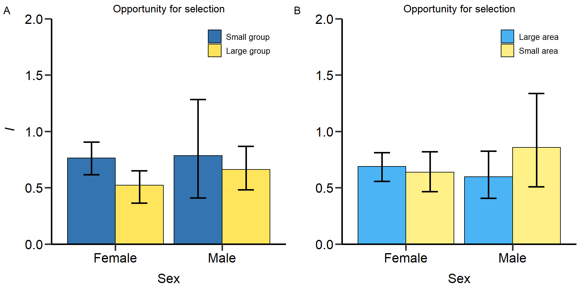 Figure 7: Effects of group size (A) and area treatment (B) on the
opportunity for selection (variance in reproductive success) in females
and males. Means and 95% confidence intervals.
Figure 7: Effects of group size (A) and area treatment (B) on the
opportunity for selection (variance in reproductive success) in females
and males. Means and 95% confidence intervals.
Treatement
comparisons via permutation test for the opportunity for selection
Table_BatemanMetrics_TreatComp_round[c(1,5,9,13),c(1,3,4,5,6)] Sex Selection_metric Variance l95.CI u95.CI
1 Male Opportunity for selection -0.261 -0.778 0.161
5 Male Opportunity for selection 0.124 -0.310 0.653
9 Female Opportunity for selection 0.050 -0.170 0.258
13 Female Opportunity for selection 0.240 0.043 0.450Sex comparisons via permutation test for the opportunity for selection
Table_BatemanMetrics_SexComp_round[c(1,5,9,13),c(1,3,4,5,6)] Treatment Variance l95.CI u95.CI p-value
1 Small group size 0.023 -0.383 0.534 0.859
5 Large group size 0.140 -0.087 0.390 0.136
9 Large area -0.091 -0.322 0.172 0.281
13 Small area 0.220 -0.184 0.723 0.199Opportunity for sexual selection
# Opportunity for sexual selection
BarPlot_3<- ggplot(Table_BatemanMetrics_pop[c(3,4,11,12),], aes(x=Sex, y=Variance, fill=Treatment)) +
scale_y_continuous(limits = c(0,1), breaks = seq(0,1,0.25), expand = c(0 ,0)) +
geom_hline(yintercept=0, linetype="dashed", color = "black", size=1) +
geom_bar(stat="identity", color="black", position=position_dodge(), alpha=0.8) +
ylab(expression(paste(~italic("I"['s']))))+ggtitle('Opportunity for sexual selection')+labs(tag = "A")+xlab('Sex')+
scale_x_discrete(breaks=waiver(),labels = c("Female","Male"))+
theme(panel.border = element_blank(),
plot.title = element_text(hjust = 0.5),
panel.background = element_blank(),
panel.grid.major = element_blank(),
panel.grid.minor = element_blank(),
plot.tag.position=c(0.01,0.98),
legend.position = c(0.8, 0.9),
legend.title = element_blank(),
legend.text = element_text(colour="black", size=10),
axis.line.x = element_line(colour = "black", size = 1),
axis.line.y = element_line(colour = "black", size = 1),
axis.text.x = element_text(face="plain", color="black", size=16, angle=0),
axis.text.y = element_text(face="plain", color="black", size=16, angle=0),
axis.title.x = element_text(size=16,face="plain", margin = margin(r=0,10,0,0)),
axis.title.y = element_text(size=16,face="plain", margin = margin(r=10,0,0,0)),
axis.ticks = element_line(size = 1),
axis.ticks.length = unit(.3, "cm")) +
geom_errorbar(aes(ymin=l95.CI, ymax=u95.CI), width=.3,size=1, position=position_dodge(.9)) +
scale_fill_manual(values=c(colorESEB[1],colorESEB[2]),name = "Treatment", labels = c('Small group','Large group'))
BarPlot_4<- ggplot(Table_BatemanMetrics_area[c(3,4,11,12),], aes(x=Sex, y=Variance, fill=Treatment)) +
scale_y_continuous(limits = c(0,1), breaks = seq(0,1,0.25), expand = c(0 ,0)) +
geom_hline(yintercept=0, linetype="dashed", color = "black", size=1) +
geom_bar(stat="identity", color="black", position=position_dodge(), alpha=0.8) +
ylab('')+ggtitle('Opportunity for sexual selection')+labs(tag = "B")+xlab('Sex')+
scale_x_discrete(breaks=waiver(),labels = c("Female","Male"))+
theme(panel.border = element_blank(),
plot.title = element_text(hjust = 0.5),
panel.background = element_blank(),
panel.grid.major = element_blank(),
panel.grid.minor = element_blank(),
plot.tag.position=c(0.01,0.98),
legend.position = c(0.8, 0.9),
legend.title = element_blank(),
legend.text = element_text(colour="black", size=10),
axis.line.x = element_line(colour = "black", size = 1),
axis.line.y = element_line(colour = "black", size = 1),
axis.text.x = element_text(face="plain", color="black", size=16, angle=0),
axis.text.y = element_text(face="plain", color="black", size=16, angle=0),
axis.title.x = element_text(size=16,face="plain", margin = margin(r=0,10,0,0)),
axis.title.y = element_text(size=16,face="plain", margin = margin(r=10,0,0,0)),
axis.ticks = element_line(size = 1),
axis.ticks.length = unit(.3, "cm")) +
geom_errorbar(aes(ymin=l95.CI, ymax=u95.CI), width=.3,size=1, position=position_dodge(.9)) +
scale_fill_manual(values=c(colorESEB2[1],colorESEB2[2]),name = "Treatment", labels = c('Large area','Small area'))
grid.arrange(grobs = list(BarPlot_3,BarPlot_4), nrow = 1,ncol=2, widths=c(2.3, 2.3))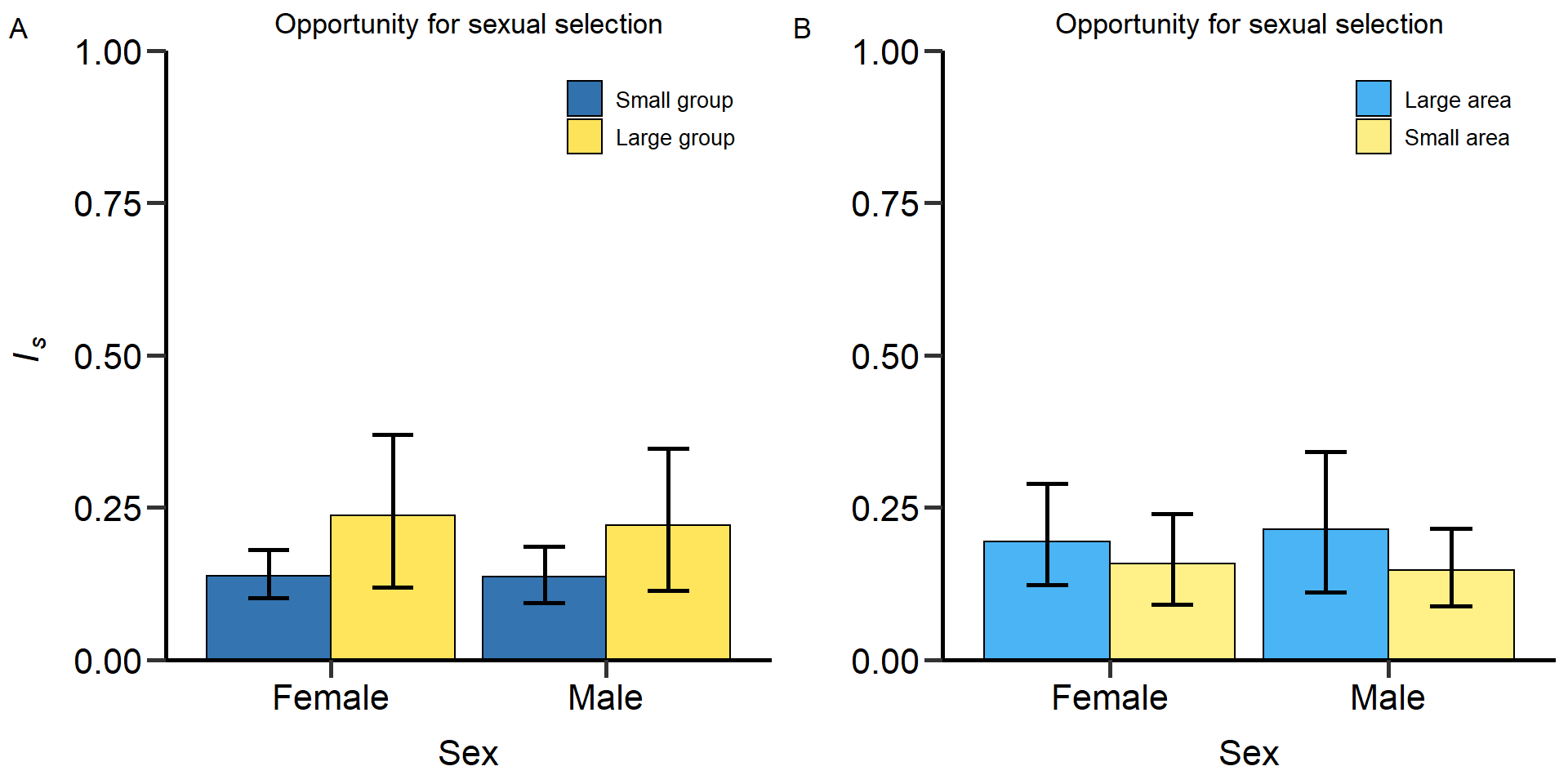 Figure 8: Effects of group size (A) and area treatment (B) on the
opportunity for sexual selection (variance in mating success) in females
and males. Means and 95% confidence intervals.
Figure 8: Effects of group size (A) and area treatment (B) on the
opportunity for sexual selection (variance in mating success) in females
and males. Means and 95% confidence intervals.
Treatement
comparisons via permutation test for the opportunity for sexual
selection
Table_BatemanMetrics_TreatComp_round[c(2,6,10,14),c(1,3,4,5,6)] Sex Selection_metric Variance l95.CI u95.CI
2 Male Opportunity for sexual selection 0.067 -0.055 0.206
6 Male Opportunity for sexual selection -0.084 -0.216 0.033
10 Female Opportunity for sexual selection 0.036 -0.075 0.155
14 Female Opportunity for sexual selection -0.099 -0.235 0.025Sex comparisons via permutation test for the opportunity for selection
Table_BatemanMetrics_SexComp_round[c(2,6,10,14),c(1,3,4,5,6)] Treatment Variance l95.CI u95.CI p-value
2 Small group size -0.001 -0.064 0.059 0.960
6 Large group size -0.016 -0.187 0.153 0.770
10 Large area 0.020 -0.119 0.172 0.689
14 Small area -0.011 -0.111 0.086 0.718Bateman gradient
# Bateman gradient
BarPlot_5<- ggplot(Table_BatemanMetrics_pop[c(5,6,13,14),], aes(x=Sex, y=Variance, fill=Treatment)) +
geom_hline(yintercept=0, linetype="dashed", color = "black", size=1) +
geom_bar(stat="identity", color="black", position=position_dodge(), alpha=0.8) +
ylab(expression(paste(~italic(symbol("b")['ss']))))+ggtitle('Bateman gradient')+labs(tag = "A")+xlab('Sex')+
scale_x_discrete(breaks=waiver(),labels = c("Female","Male"))+
theme(panel.border = element_blank(),
plot.title = element_text(hjust = 0.5),
panel.background = element_blank(),
panel.grid.major = element_blank(),
panel.grid.minor = element_blank(),
plot.tag.position=c(0.01,0.98),
legend.position = c(0.8, 0.9),
legend.title = element_blank(),
legend.text = element_text(colour="black", size=10),
axis.line.x = element_line(colour = "black", size = 1),
axis.line.y = element_line(colour = "black", size = 1),
axis.text.x = element_text(face="plain", color="black", size=16, angle=0),
axis.text.y = element_text(face="plain", color="black", size=16, angle=0),
axis.title.x = element_text(size=16,face="plain", margin = margin(r=0,10,0,0)),
axis.title.y = element_text(size=16,face="plain", margin = margin(r=10,0,0,0)),
axis.ticks = element_line(size = 1),
axis.ticks.length = unit(.3, "cm")) +
geom_errorbar(aes(ymin=l95.CI, ymax=u95.CI), width=.3,size=1, position=position_dodge(.9)) +
scale_fill_manual(values=c(colorESEB[1],colorESEB[2]),name = "Treatment", labels = c('Small group','Large group'))
BarPlot_6<- ggplot(Table_BatemanMetrics_area[c(5,6,13,14),], aes(x=Sex, y=Variance, fill=Treatment)) +
geom_hline(yintercept=0, linetype="dashed", color = "black", size=1) +
geom_bar(stat="identity", color="black", position=position_dodge(), alpha=0.8) +
ylab('')+ggtitle('Bateman gradient')+labs(tag = "B")+xlab('Sex')+
scale_x_discrete(breaks=waiver(),labels = c("Female","Male"))+
theme(panel.border = element_blank(),
plot.title = element_text(hjust = 0.5),
panel.background = element_blank(),
panel.grid.major = element_blank(),
panel.grid.minor = element_blank(),
plot.tag.position=c(0.01,0.98),
legend.position = c(0.8, 0.9),
legend.title = element_blank(),
legend.text = element_text(colour="black", size=10),
axis.line.x = element_line(colour = "black", size = 1),
axis.line.y = element_line(colour = "black", size = 1),
axis.text.x = element_text(face="plain", color="black", size=16, angle=0),
axis.text.y = element_text(face="plain", color="black", size=16, angle=0),
axis.title.x = element_text(size=16,face="plain", margin = margin(r=0,10,0,0)),
axis.title.y = element_text(size=16,face="plain", margin = margin(r=10,0,0,0)),
axis.ticks = element_line(size = 1),
axis.ticks.length = unit(.3, "cm")) +
geom_errorbar(aes(ymin=l95.CI, ymax=u95.CI), width=.3,size=1, position=position_dodge(.9)) +
scale_fill_manual(values=c(colorESEB2[1],colorESEB2[2]),name = "Treatment", labels = c('Large area','Small area'))
grid.arrange(grobs = list(BarPlot_5,BarPlot_6), nrow = 1,ncol=2, widths=c(2.3, 2.3))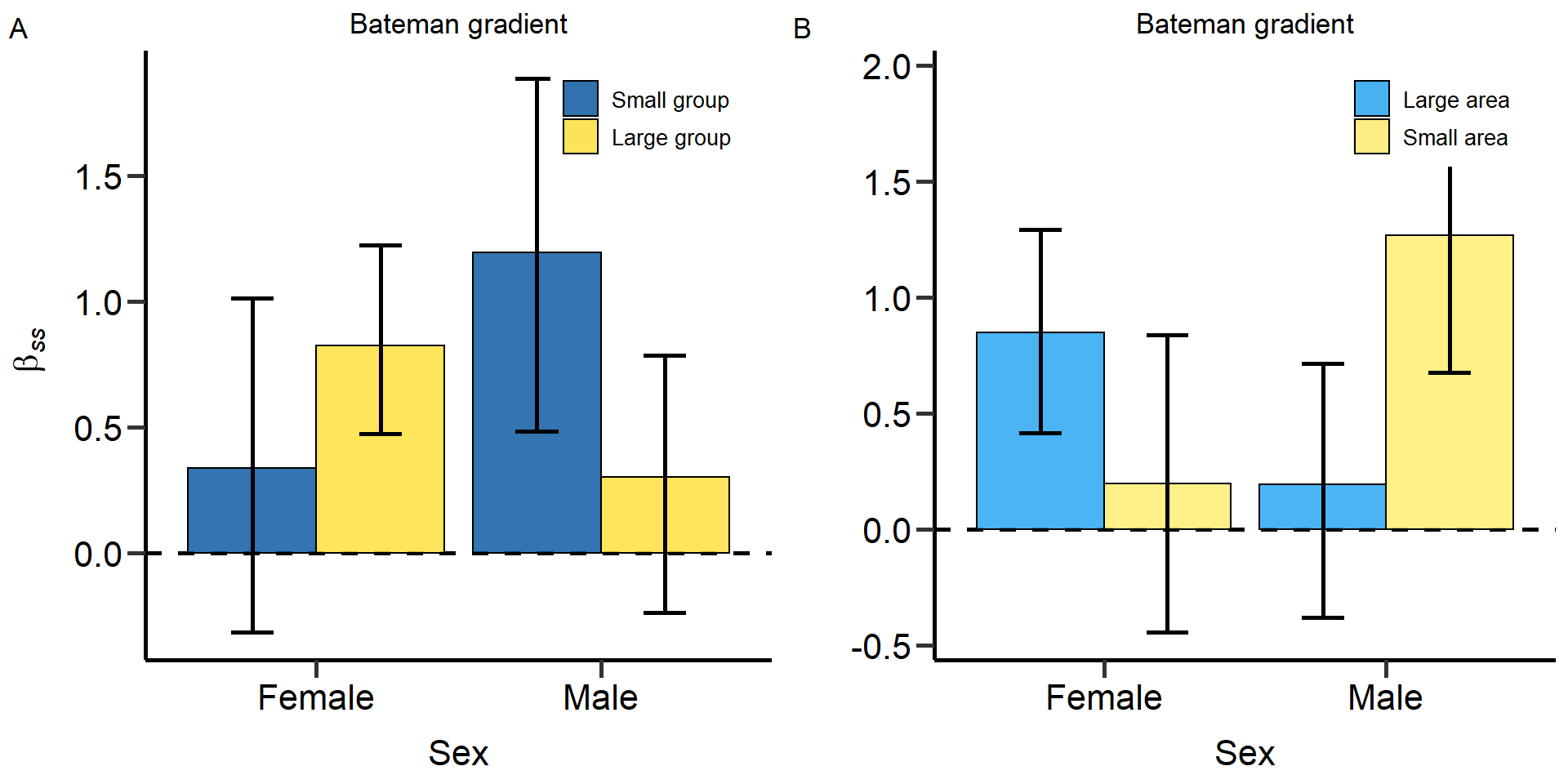 Figure 9: Effects of group size (A) and area treatment (B) on the
Bateman gradient (slope of mating success on reproductive success) in
females and males. Means and 95% confidence intervals.
Figure 9: Effects of group size (A) and area treatment (B) on the
Bateman gradient (slope of mating success on reproductive success) in
females and males. Means and 95% confidence intervals.
Treatement comparisons via permutation test for the Bateman gradient
Table_BatemanMetrics_TreatComp_round[c(3,7,11,15),c(1,3,4,5,6)] Sex Selection_metric Variance l95.CI u95.CI
3 Male Bateman gradient -1.074 -1.954 -0.270
7 Male Bateman gradient 0.892 0.025 1.754
11 Female Bateman gradient 0.653 -0.124 1.410
15 Female Bateman gradient -0.485 -1.258 0.277Sex comparisons via permutation test for the opportunity for selection
Table_BatemanMetrics_SexComp_round[c(3,7,11,15),c(1,3,4,5,6)] Treatment Variance l95.CI u95.CI p-value
3 Small group size 0.854 -0.125 1.805 0.012
7 Large group size -0.523 -1.180 0.077 0.052
11 Large area -0.655 -1.363 0.025 0.021
15 Small area 1.072 0.181 2.011 0.003# Bateman gradient (scatter)
p1<-ggplot(DB_data_clean_Small_pop, aes(x=rel_m_cMS, y=rel_m_RS)) +
geom_point(alpha=0.4,shape=16, size = 3,color=colpal2[2]) +
geom_smooth(method=lm, se=TRUE,alpha=0.3) +
theme(plot.tag.position=c(0.1,0.98))+
labs(tag = "A")+xlab('Rel. mating success')+ylab("Rel. reproductive success")+ggtitle('Small group')+ theme(plot.title = element_text(hjust = 0.5))+
theme(axis.text=element_text(size=13),
axis.title=element_text(size=14))+ theme(legend.position="none")+
ylim(0,4.2)+xlim(0,3.2)+
annotate("text",label=expression(paste(beta['female'],' = 0.69')),x=.48,y=4.2,size=4)+
annotate("text",label=expression(paste(beta['male'],' = 1.15')),x=.42,y=3.85,size=4)+
theme(panel.grid.major = element_blank(), panel.grid.minor = element_blank(),panel.background = element_blank(), axis.line = element_line(colour = "black"))
p1=p1+geom_point(aes(x=rel_f_cMS, y=rel_f_RS),color=colpal2[1],alpha=0.4,shape=16, size = 3)+
geom_smooth(aes(x=rel_f_cMS, y=rel_f_RS),color=colpal2[1],method=lm, se=TRUE,alpha=0.3)
p2<-ggplot(DB_data_clean_Large_pop, aes(x=rel_m_cMS, y=rel_m_RS)) +
geom_point(alpha=0.4,shape=16, size = 3,color=colpal2[2]) +
geom_smooth(method=lm, se=TRUE,alpha=0.3) +
theme(plot.tag.position=c(0.1,0.98))+
labs(tag = "B")+xlab('Rel. mating success')+ylab("Rel. reproductive success")+ggtitle('Large group')+ theme(plot.title = element_text(hjust = 0.5))+
theme(axis.text=element_text(size=13),
axis.title=element_text(size=14))+ theme(legend.position="none")+
ylim(0,4.2)+xlim(0,3.2)+
annotate("text",label=expression(paste(beta['female'],' = 0.88')),x=.48,y=4.2,size=4)+
annotate("text",label=expression(paste(beta['male'],' = 0.59')),x=.42,y=3.85,size=4)+
theme(panel.grid.major = element_blank(), panel.grid.minor = element_blank(),panel.background = element_blank(), axis.line = element_line(colour = "black"))
p2=p2+geom_point(aes(x=rel_f_cMS, y=rel_f_RS),color=colpal2[1],alpha=0.4,shape=16, size = 3)+
geom_smooth(aes(x=rel_f_cMS, y=rel_f_RS),color=colpal2[1],method=lm, se=TRUE,alpha=0.3)
p3<-ggplot(DB_data_clean_Large_area, aes(x=rel_m_cMS, y=rel_m_RS)) +
geom_point(alpha=0.4,shape=16, size = 3,color=colpal2[2]) +
geom_smooth(method=lm, se=TRUE,alpha=0.3) +
theme(plot.tag.position=c(0.1,0.98))+
labs(tag = "C")+xlab('Rel. mating success')+ylab("Rel. reproductive success")+ggtitle('Large area')+ theme(plot.title = element_text(hjust = 0.5))+
theme(axis.text=element_text(size=13),
axis.title=element_text(size=14))+ theme(legend.position="none")+
ylim(0,4.2)+xlim(0,3.2)+
annotate("text",label=expression(paste(beta['female'],' = 0.93')),x=.48,y=4.2,size=4)+
annotate("text",label=expression(paste(beta['male'],' = 0.51')),x=.42,y=3.85,size=4)+
theme(panel.grid.major = element_blank(), panel.grid.minor = element_blank(),panel.background = element_blank(), axis.line = element_line(colour = "black"))
p3=p3+geom_point(aes(x=rel_f_cMS, y=rel_f_RS),color=colpal2[1],alpha=0.4,shape=16, size = 3)+
geom_smooth(aes(x=rel_f_cMS, y=rel_f_RS),color=colpal2[1],method=lm, se=TRUE,alpha=0.3)
p4<-ggplot(DB_data_clean_Small_area, aes(x=rel_m_cMS, y=rel_m_RS)) +
geom_point(alpha=0.4,shape=16, size = 3,color=colpal2[2]) +
geom_smooth(method=lm, se=TRUE,alpha=0.3) +
theme(plot.tag.position=c(0.1,0.98))+
labs(tag = "D")+xlab('Rel. mating success')+ylab("Rel. reproductive success")+ggtitle('Small area')+ theme(plot.title = element_text(hjust = 0.5))+
theme(axis.text=element_text(size=13),
axis.title=element_text(size=14))+
ylim(0,4.2)+xlim(0,3.2)+
theme(legend.position="none")+
annotate("text",label=expression(paste(beta['female'],' = 0.72')),x=.48,y=4.2,size=4)+
annotate("text",label=expression(paste(beta['male'],' = 1.19')),x=.42,y=3.85,size=4)+
theme(panel.grid.major = element_blank(), panel.grid.minor = element_blank(),panel.background = element_blank(), axis.line = element_line(colour = "black"))
p4=p4+geom_point(aes(x=rel_f_cMS, y=rel_f_RS),color=colpal2[1],alpha=0.4,shape=16, size = 3)+
geom_smooth(aes(x=rel_f_cMS, y=rel_f_RS),color=colpal2[1],method=lm, se=TRUE,alpha=0.3)
#Create legend
p5<-ggplot(DB_data_clean, aes(x=Total_N_MTP1, y=Total_N_Rd, color=Sex)) +
geom_point(alpha=0.4,shape=16, size = 3, position=position_jitterdodge(jitter.height=0,jitter.width=0,dodge.width = 0)) +
geom_smooth(method=lm, se=TRUE,alpha=0.3) +
scale_color_manual(values=c(colpal2[1],colpal2[2]),name = "Sex", labels = c('Females','Males'))+
xlab('Rel. mating success')+ylab("Rel. reproductive success")+
guides(color=guide_legend(override.aes=list(fill=NA)))+
theme(legend.key = element_rect(fill = "transparent"))
legend <- get_legend(p5)
plot1<-grid.arrange(p1,p2,legend,p3,p4,legend, nrow = 2,ncol=3, widths=c(2.3, 2.3, 0.65))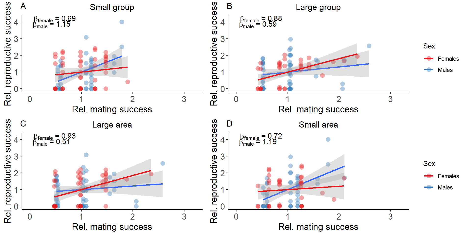 Figure 10: Scatter plot of the Bateman gradient in females and males.
Means and 95% confidence intervals.
Figure 10: Scatter plot of the Bateman gradient in females and males.
Means and 95% confidence intervals.
Jones index
# Jones index
BarPlot_7<- ggplot(Table_BatemanMetrics_pop[c(7,8,14,15),], aes(x=Sex, y=Variance, fill=Treatment)) +
geom_hline(yintercept=0, linetype="dashed", color = "black", size=1) +
geom_bar(stat="identity", color="black", position=position_dodge(), alpha=0.8) +
ylab(expression(paste(~italic("s'"['max']))))+ggtitle('Jones index')+labs(tag = "A")+xlab('Sex')+
scale_x_discrete(breaks=waiver(),labels = c("Female","Male"))+
theme(panel.border = element_blank(),
plot.title = element_text(hjust = 0.5),
panel.background = element_blank(),
panel.grid.major = element_blank(),
panel.grid.minor = element_blank(),
plot.tag.position=c(0.01,0.98),
legend.position = c(0.8, 0.9),
legend.title = element_blank(),
legend.text = element_text(colour="black", size=10),
axis.line.x = element_line(colour = "black", size = 1),
axis.line.y = element_line(colour = "black", size = 1),
axis.text.x = element_text(face="plain", color="black", size=16, angle=0),
axis.text.y = element_text(face="plain", color="black", size=16, angle=0),
axis.title.x = element_text(size=16,face="plain", margin = margin(r=0,10,0,0)),
axis.title.y = element_text(size=16,face="plain", margin = margin(r=10,0,0,0)),
axis.ticks = element_line(size = 1),
axis.ticks.length = unit(.3, "cm")) +
geom_errorbar(aes(ymin=l95.CI, ymax=u95.CI), width=.3,size=1, position=position_dodge(.9)) +
scale_fill_manual(values=c(colorESEB[1],colorESEB[2]),name = "Treatment", labels = c('Small group','Large group'))
BarPlot_8<- ggplot(Table_BatemanMetrics_area[c(7,8,14,15),], aes(x=Sex, y=Variance, fill=Treatment)) +
geom_hline(yintercept=0, linetype="dashed", color = "black", size=1) +
geom_bar(stat="identity", color="black", position=position_dodge(), alpha=0.8) +
ylab('')+ggtitle('Jones index')+labs(tag = "B")+xlab('Sex')+
scale_x_discrete(breaks=waiver(),labels = c("Female","Male"))+
theme(panel.border = element_blank(),
plot.title = element_text(hjust = 0.5),
panel.background = element_blank(),
panel.grid.major = element_blank(),
panel.grid.minor = element_blank(),
plot.tag.position=c(0.01,0.98),
legend.position = c(0.8, 0.9),
legend.title = element_blank(),
legend.text = element_text(colour="black", size=10),
axis.line.x = element_line(colour = "black", size = 1),
axis.line.y = element_line(colour = "black", size = 1),
axis.text.x = element_text(face="plain", color="black", size=16, angle=0),
axis.text.y = element_text(face="plain", color="black", size=16, angle=0),
axis.title.x = element_text(size=16,face="plain", margin = margin(r=0,10,0,0)),
axis.title.y = element_text(size=16,face="plain", margin = margin(r=10,0,0,0)),
axis.ticks = element_line(size = 1),
axis.ticks.length = unit(.3, "cm")) +
geom_errorbar(aes(ymin=l95.CI, ymax=u95.CI), width=.3,size=1, position=position_dodge(.9)) +
scale_fill_manual(values=c(colorESEB2[1],colorESEB2[2]),name = "Treatment", labels = c('Large area','Small area'))
grid.arrange(grobs = list(BarPlot_7,BarPlot_8), nrow = 1,ncol=2, widths=c(2.3, 2.3))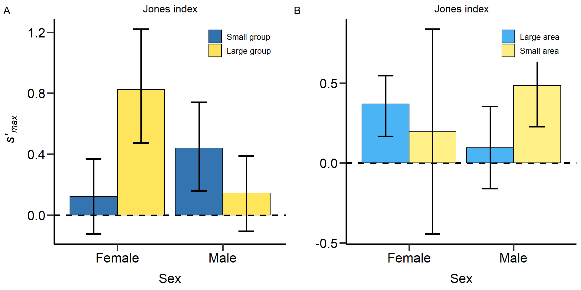 Figure 11: Effects of group size (A) and area treatment (B) on the Jones
index (maximum strength of sexual selection) in females and males. Means
and 95% confidence intervals.
Figure 11: Effects of group size (A) and area treatment (B) on the Jones
index (maximum strength of sexual selection) in females and males. Means
and 95% confidence intervals.
Treatement comparisons via
permutation test for the Jones index
Table_BatemanMetrics_TreatComp_round[c(4,8,12,16),c(1,3,4,5,6)] Sex Selection_metric Variance l95.CI u95.CI
4 Male Jones index -0.389 -0.777 -0.009
8 Male Jones index 0.297 -0.075 0.694
12 Female Jones index 0.290 -0.026 0.600
16 Female Jones index -0.269 -0.563 0.035Sex comparisons via permutation test for the opportunity for selection
Table_BatemanMetrics_SexComp_round[c(4,8,12,16),c(1,3,4,5,6)] Treatment Variance l95.CI u95.CI p-value
4 Small group size 0.319 -0.060 0.712 0.011
8 Large group size -0.246 -0.542 0.053 0.039
12 Large area -0.273 -0.593 0.057 0.018
16 Small area 0.406 0.046 0.780 0.002Variance decopmposition
We decomposed the variance in reproductive success for males and
females.
Components fro males were:
- Mating success
-
Insemination success
- Fertilization success
- Partner
fecundity
Components for females were:
- Mating success
- Fecundity
We used bootstrapping (10.000 bootstrap
replicates) to obtain 95% confidence intervals and permutation tests
(10.000 permutations) to statistically compare treatments and
sexes.
# Bootstrapping variances + CI
# mMS
# Large area
DB_data_clean_Large_area_M_MS_n <-as.data.table(DB_data_clean_Large_area$rel_m_cMS)
c <- function(d, i){
  d2 <- d[i,]
  return(var(d2[,1], na.rm=TRUE))
}
Large_area_M_MS_bootvar <- boot(DB_data_clean_Large_area_M_MS_n, c, R=10000)


# Small Area
DB_data_clean_Small_area_M_MS_n <-as.data.table(DB_data_clean_Small_area$rel_m_cMS)

Small_area_M_MS_bootvar <- boot(DB_data_clean_Small_area_M_MS_n, c, R=10000)


# Small group
DB_data_clean_Small_pop_M_MS_n <-as.data.table(DB_data_clean_Small_pop$rel_m_cMS)

Small_pop_M_MS_bootvar <- boot(DB_data_clean_Small_pop_M_MS_n, c, R=10000)


# Large group
DB_data_clean_Large_pop_M_MS_n <-as.data.table(DB_data_clean_Large_pop$rel_m_cMS)

Large_pop_M_MS_bootvar <- boot(DB_data_clean_Large_pop_M_MS_n, c, R=10000)

rm("c")

# InSuc ####
# Large area
DB_data_clean_Large_area_M_InSuc_n <-as.data.table(DB_data_clean_Large_area$rel_m_InSuc)
c <- function(d, i){
  d2 <- d[i,]
  return(var(d2[,1], na.rm=TRUE))
}
Large_area_M_InSuc_bootvar <- boot(DB_data_clean_Large_area_M_InSuc_n, c, R=10000)


# Small Area
DB_data_clean_Small_area_M_InSuc_n <-as.data.table(DB_data_clean_Small_area$rel_m_InSuc)

Small_area_M_InSuc_bootvar <- boot(DB_data_clean_Small_area_M_InSuc_n, c, R=10000)


# Small group
DB_data_clean_Small_pop_M_InSuc_n <-as.data.table(DB_data_clean_Small_pop$rel_m_InSuc)

Small_pop_M_InSuc_bootvar <- boot(DB_data_clean_Small_pop_M_InSuc_n, c, R=10000)


# Large group
DB_data_clean_Large_pop_M_InSuc_n <-as.data.table(DB_data_clean_Large_pop$rel_m_InSuc)

Large_pop_M_InSuc_bootvar <- boot(DB_data_clean_Large_pop_M_InSuc_n, c, R=10000)

rm("c")

# feSuc ####
# Large area
DB_data_clean_Large_area_M_feSuc_n <-as.data.table(DB_data_clean_Large_area$rel_m_feSuc)
c <- function(d, i){
  d2 <- d[i,]
  return(var(d2$V1, na.rm=TRUE))
}
Large_area_M_feSuc_bootvar <- boot(DB_data_clean_Large_area_M_feSuc_n, c, R=10000)


# Small Area
DB_data_clean_Small_area_M_feSuc_n <-as.data.table(DB_data_clean_Small_area$rel_m_feSuc)

Small_area_M_feSuc_bootvar <- boot(DB_data_clean_Small_area_M_feSuc_n, c, R=10000)

# Small group
DB_data_clean_Small_pop_M_feSuc_n <-as.data.table(DB_data_clean_Small_pop$rel_m_feSuc)

Small_pop_M_feSuc_bootvar <- boot(DB_data_clean_Small_pop_M_feSuc_n, c, R=10000)


# Large group
DB_data_clean_Large_pop_M_feSuc_n <-as.data.table(DB_data_clean_Large_pop$rel_m_feSuc)

Large_pop_M_feSuc_bootvar <- boot(DB_data_clean_Large_pop_M_feSuc_n, c, R=10000)

rm("c")

# pFec ####
# Large area
DB_data_clean_Large_area_M_pFec_n <-as.data.table(DB_data_clean_Large_area$rel_m_pFec)
c <- function(d, i){
  d2 <- d[i,]
  return(var(d2[,1], na.rm=TRUE))
}
Large_area_M_pFec_bootvar <- boot(DB_data_clean_Large_area_M_pFec_n, c, R=10000)


# Small Area
DB_data_clean_Small_area_M_pFec_n <-as.data.table(DB_data_clean_Small_area$rel_m_pFec)

Small_area_M_pFec_bootvar <- boot(DB_data_clean_Small_area_M_pFec_n, c, R=10000)


# Small group
DB_data_clean_Small_pop_M_pFec_n <-as.data.table(DB_data_clean_Small_pop$rel_m_pFec)

Small_pop_M_pFec_bootvar <- boot(DB_data_clean_Small_pop_M_pFec_n, c, R=10000)

# Large group
DB_data_clean_Large_pop_M_pFec_n <-as.data.table(DB_data_clean_Large_pop$rel_m_pFec)

Large_pop_M_pFec_bootvar <- boot(DB_data_clean_Large_pop_M_pFec_n, c, R=10000)

rm("c")

# fMS ####
# Large area
DB_data_clean_Large_area_F_fMS_n <-as.data.table(DB_data_clean_Large_area$rel_f_cMS)
c <- function(d, i){
  d2 <- d[i,]
  return(var(d2[,1], na.rm=TRUE))
}
Large_area_F_fMS_bootvar <- boot(DB_data_clean_Large_area_F_fMS_n, c, R=10000)


# Small Area
DB_data_clean_Small_area_F_fMS_n <-as.data.table(DB_data_clean_Small_area$rel_f_cMS)

Small_area_F_fMS_bootvar <- boot(DB_data_clean_Small_area_F_fMS_n, c, R=10000)


# Small group
DB_data_clean_Small_pop_F_fMS_n <-as.data.table(DB_data_clean_Small_pop$rel_f_cMS)

Small_pop_F_fMS_bootvar <- boot(DB_data_clean_Small_pop_F_fMS_n, c, R=10000)


# Large group
DB_data_clean_Large_pop_F_fMS_n <-as.data.table(DB_data_clean_Large_pop$rel_f_cMS)

Large_pop_F_fMS_bootvar <- boot(DB_data_clean_Large_pop_F_fMS_n, c, R=10000)

rm("c")

# fFec ####
# Large area
DB_data_clean_Large_area_F_fFec_n <-as.data.table(DB_data_clean_Large_area$rel_f_fec_pMate)
c <- function(d, i){
  d2 <- d[i,]
  return(var(d2[,1], na.rm=TRUE))
}
Large_area_F_fFec_bootvar <- boot(DB_data_clean_Large_area_F_fFec_n, c, R=10000)


# Small Area
DB_data_clean_Small_area_F_fFec_n <-as.data.table(DB_data_clean_Small_area$rel_f_fec_pMate)

Small_area_F_fFec_bootvar <- boot(DB_data_clean_Small_area_F_fFec_n, c, R=10000)


# Small group
DB_data_clean_Small_pop_F_fFec_n <-as.data.table(DB_data_clean_Small_pop$rel_f_fec_pMate)

Small_pop_F_fFec_bootvar <- boot(DB_data_clean_Small_pop_F_fFec_n, c, R=10000)

# Large group
DB_data_clean_Large_pop_F_fFec_n <-as.data.table(DB_data_clean_Large_pop$rel_f_fec_pMate)

Large_pop_F_fFec_bootvar <- boot(DB_data_clean_Large_pop_F_fFec_n, c, R=10000)

rm("c")

#Write Table ####
library(base)

PhenVarBoot_Table_Male_Large_area_MS <- as.data.frame(cbind("Male", "MS", "Large_area", mean(Large_area_M_MS_bootvar$t), quantile(Large_area_M_MS_bootvar$t,.025, names = FALSE), quantile(Large_area_M_MS_bootvar$t,.975, names = FALSE)))
PhenVarBoot_Table_Male_Small_area_MS <- as.data.frame(cbind("Male", "MS", "Small_area", mean(Small_area_M_MS_bootvar$t), quantile(Small_area_M_MS_bootvar$t,.025, names = FALSE), quantile(Small_area_M_MS_bootvar$t,.975, names = FALSE)))
PhenVarBoot_Table_Male_Small_pop_MS <- as.data.frame(cbind("Male", "MS", "Small_pop", mean(Small_pop_M_MS_bootvar$t), quantile(Small_pop_M_MS_bootvar$t,.025, names = FALSE), quantile(Small_pop_M_MS_bootvar$t,.975, names = FALSE)))
PhenVarBoot_Table_Male_Large_pop_MS <- as.data.frame(cbind("Male", "MS", "Large_pop", mean(Large_pop_M_MS_bootvar$t), quantile(Large_pop_M_MS_bootvar$t,.025, names = FALSE), quantile(Large_pop_M_MS_bootvar$t,.975, names = FALSE)))

PhenVarBoot_Table_Male_Large_area_InSuc <- as.data.frame(cbind("Male", "InSuc", "Large_area", mean(Large_area_M_InSuc_bootvar$t), quantile(Large_area_M_InSuc_bootvar$t,.025, names = FALSE), quantile(Large_area_M_InSuc_bootvar$t,.975, names = FALSE)))
PhenVarBoot_Table_Male_Small_area_InSuc <- as.data.frame(cbind("Male", "InSuc", "Small_area", mean(Small_area_M_InSuc_bootvar$t), quantile(Small_area_M_InSuc_bootvar$t,.025, names = FALSE), quantile(Small_area_M_InSuc_bootvar$t,.975, names = FALSE)))
PhenVarBoot_Table_Male_Small_pop_InSuc <- as.data.frame(cbind("Male", "InSuc", "Small_pop", mean(Small_pop_M_InSuc_bootvar$t), quantile(Small_pop_M_InSuc_bootvar$t,.025, names = FALSE), quantile(Small_pop_M_InSuc_bootvar$t,.975, names = FALSE)))
PhenVarBoot_Table_Male_Large_pop_InSuc <- as.data.frame(cbind("Male", "InSuc", "Large_pop", mean(Large_pop_M_InSuc_bootvar$t), quantile(Large_pop_M_InSuc_bootvar$t,.025, names = FALSE), quantile(Large_pop_M_InSuc_bootvar$t,.975, names = FALSE)))

PhenVarBoot_Table_Male_Large_area_feSuc <- as.data.frame(cbind("Male", "feSuc", "Large_area", mean(Large_area_M_feSuc_bootvar$t), quantile(Large_area_M_feSuc_bootvar$t,.025, names = FALSE), quantile(Large_area_M_feSuc_bootvar$t,.975, names = FALSE)))
PhenVarBoot_Table_Male_Small_area_feSuc <- as.data.frame(cbind("Male", "feSuc", "Small_area", mean(Small_area_M_feSuc_bootvar$t), quantile(Small_area_M_feSuc_bootvar$t,.025, names = FALSE), quantile(Small_area_M_feSuc_bootvar$t,.975, names = FALSE)))
PhenVarBoot_Table_Male_Small_pop_feSuc <- as.data.frame(cbind("Male", "feSuc", "Small_pop", mean(Small_pop_M_feSuc_bootvar$t), quantile(Small_pop_M_feSuc_bootvar$t,.025, names = FALSE), quantile(Small_pop_M_feSuc_bootvar$t,.975, names = FALSE)))
PhenVarBoot_Table_Male_Large_pop_feSuc <- as.data.frame(cbind("Male", "feSuc", "Large_pop", mean(Large_pop_M_feSuc_bootvar$t), quantile(Large_pop_M_feSuc_bootvar$t,.025, names = FALSE), quantile(Large_pop_M_feSuc_bootvar$t,.975, names = FALSE)))

PhenVarBoot_Table_Male_Large_area_pFec <- as.data.frame(cbind("Male", "pFec", "Large_area", mean(Large_area_M_pFec_bootvar$t), quantile(Large_area_M_pFec_bootvar$t,.025, names = FALSE), quantile(Large_area_M_pFec_bootvar$t,.975, names = FALSE)))
PhenVarBoot_Table_Male_Small_area_pFec <- as.data.frame(cbind("Male", "pFec", "Small_area", mean(Small_area_M_pFec_bootvar$t), quantile(Small_area_M_pFec_bootvar$t,.025, names = FALSE), quantile(Small_area_M_pFec_bootvar$t,.975, names = FALSE)))
PhenVarBoot_Table_Male_Small_pop_pFec <- as.data.frame(cbind("Male", "pFec", "Small_pop", mean(Small_pop_M_pFec_bootvar$t), quantile(Small_pop_M_pFec_bootvar$t,.025, names = FALSE), quantile(Small_pop_M_pFec_bootvar$t,.975, names = FALSE)))
PhenVarBoot_Table_Male_Large_pop_pFec <- as.data.frame(cbind("Male", "pFec", "Large_pop", mean(Large_pop_M_pFec_bootvar$t), quantile(Large_pop_M_pFec_bootvar$t,.025, names = FALSE), quantile(Large_pop_M_pFec_bootvar$t,.975, names = FALSE)))

PhenVarBoot_Table_Female_Large_area_fMS <- as.data.frame(cbind("Female", "fMS", "Large_area", mean(Large_area_F_fMS_bootvar$t), quantile(Large_area_F_fMS_bootvar$t,.025, names = FALSE), quantile(Large_area_F_fMS_bootvar$t,.975, names = FALSE)))
PhenVarBoot_Table_Female_Small_area_fMS <- as.data.frame(cbind("Female", "fMS", "Small_area", mean(Small_area_F_fMS_bootvar$t), quantile(Small_area_F_fMS_bootvar$t,.025, names = FALSE), quantile(Small_area_F_fMS_bootvar$t,.975, names = FALSE)))
PhenVarBoot_Table_Female_Small_pop_fMS <- as.data.frame(cbind("Female", "fMS", "Small_pop", mean(Small_pop_F_fMS_bootvar$t), quantile(Small_pop_F_fMS_bootvar$t,.025, names = FALSE), quantile(Small_pop_F_fMS_bootvar$t,.975, names = FALSE)))
PhenVarBoot_Table_Female_Large_pop_fMS <- as.data.frame(cbind("Female", "fMS", "Large_pop", mean(Large_pop_F_fMS_bootvar$t), quantile(Large_pop_F_fMS_bootvar$t,.025, names = FALSE), quantile(Large_pop_F_fMS_bootvar$t,.975, names = FALSE)))

PhenVarBoot_Table_Female_Large_area_fFec <- as.data.frame(cbind("Female", "fFec", "Large_area", mean(Large_area_F_fFec_bootvar$t), quantile(Large_area_F_fFec_bootvar$t,.025, names = FALSE), quantile(Large_area_F_fFec_bootvar$t,.975, names = FALSE)))
PhenVarBoot_Table_Female_Small_area_fFec <- as.data.frame(cbind("Female", "fFec", "Small_area", mean(Small_area_F_fFec_bootvar$t), quantile(Small_area_F_fFec_bootvar$t,.025, names = FALSE), quantile(Small_area_F_fFec_bootvar$t,.975, names = FALSE)))
PhenVarBoot_Table_Female_Small_pop_fFec <- as.data.frame(cbind("Female", "fFec", "Small_pop", mean(Small_pop_F_fFec_bootvar$t), quantile(Small_pop_F_fFec_bootvar$t,.025, names = FALSE), quantile(Small_pop_F_fFec_bootvar$t,.975, names = FALSE)))
PhenVarBoot_Table_Female_Large_pop_fFec <- as.data.frame(cbind("Female", "fFec", "Large_pop", mean(Large_pop_F_fFec_bootvar$t,na.rm=T), quantile(Large_pop_F_fFec_bootvar$t,.025, names = FALSE,na.rm=T), quantile(Large_pop_F_fFec_bootvar$t,.975, names = FALSE,na.rm=T)))

PhenVarBoot_Table <- as.data.frame(as.matrix(rbind(PhenVarBoot_Table_Male_Small_pop_MS,PhenVarBoot_Table_Male_Large_pop_MS,
                                                   PhenVarBoot_Table_Male_Large_area_MS,PhenVarBoot_Table_Male_Small_area_MS,
                                                   PhenVarBoot_Table_Male_Small_pop_InSuc,PhenVarBoot_Table_Male_Large_pop_InSuc,
                                                   PhenVarBoot_Table_Male_Large_area_InSuc,PhenVarBoot_Table_Male_Small_area_InSuc,
                                                   PhenVarBoot_Table_Male_Small_pop_feSuc,PhenVarBoot_Table_Male_Large_pop_feSuc,
                                                   PhenVarBoot_Table_Male_Large_area_feSuc,PhenVarBoot_Table_Male_Small_area_feSuc,
                                                   PhenVarBoot_Table_Male_Small_pop_pFec,PhenVarBoot_Table_Male_Large_pop_pFec,
                                                   PhenVarBoot_Table_Male_Large_area_pFec,PhenVarBoot_Table_Male_Small_area_pFec,
                                                   PhenVarBoot_Table_Female_Small_pop_fMS,PhenVarBoot_Table_Female_Large_pop_fMS,
                                                   PhenVarBoot_Table_Female_Large_area_fMS,PhenVarBoot_Table_Female_Small_area_fMS,
                                                   PhenVarBoot_Table_Female_Small_pop_fFec,PhenVarBoot_Table_Female_Large_pop_fFec,
                                                   PhenVarBoot_Table_Female_Large_area_fFec,PhenVarBoot_Table_Female_Small_area_fFec)))

is.table(PhenVarBoot_Table)
colnames(PhenVarBoot_Table)[1] <- "Sex"
colnames(PhenVarBoot_Table)[2] <- "Variance_component"
colnames(PhenVarBoot_Table)[3] <- "Treatment"
colnames(PhenVarBoot_Table)[4] <- "Variance"
colnames(PhenVarBoot_Table)[5] <- "l95.CI"
colnames(PhenVarBoot_Table)[6] <- "u95.CI"
PhenVarBoot_Table[,4]=as.numeric(PhenVarBoot_Table[,4])
PhenVarBoot_Table[,5]=as.numeric(PhenVarBoot_Table[,5])
PhenVarBoot_Table[,6]=as.numeric(PhenVarBoot_Table[,6])

PhenVarBoot_Table_round=cbind(PhenVarBoot_Table[,c(1,2,3)],round(PhenVarBoot_Table[,c(4,5,6)],digit=3))
rownames(PhenVarBoot_Table_round) <- NULL
# Treatment comparison
#mMS
#Area
Treat_diff_Male_area_mMS=c(Large_area_M_MS_bootvar$t)-c(Small_area_M_MS_bootvar$t)
t_Treat_diff_Male_area_mMS=mean(Treat_diff_Male_area_mMS,na.rm=TRUE)
t_Treat_diff_Male_area_mMS_lower=quantile(Treat_diff_Male_area_mMS,.025,na.rm=TRUE)
t_Treat_diff_Male_area_mMS_upper=quantile(Treat_diff_Male_area_mMS,.975,na.rm=TRUE)
#Permutation test to calculate p value
comb_data=c(DB_data_clean_Large_area$rel_m_cMS,DB_data_clean_Small_area$rel_m_cMS)
diff.observed = var(na.omit((DB_data_clean_Large_area$rel_m_cMS))) - var(na.omit((DB_data_clean_Small_area$rel_m_cMS)))
diff.observed
number_of_permutations = 100000
diff.random = NULL
for (i in 1 : number_of_permutations) {
# Sample from the combined dataset
a.random = sample (na.omit(comb_data), length(c(DB_data_clean_Large_area$rel_m_cMS)), TRUE)
b.random = sample (na.omit(comb_data), length(c(DB_data_clean_Small_area$rel_m_cMS)), TRUE)
# Null (permuated) difference
diff.random[i] = var(na.omit(b.random)) - var(na.omit(a.random))
}
# P-value is the fraction of how many times the permuted difference is
# equal or more extreme than the observed difference
t_Treat_diff_Male_area_mMS_p = sum(abs(diff.random) >= as.numeric(abs(diff.observed)))/ number_of_permutations
#Population size ####
Treat_diff_Male_pop_mMS=c(Small_pop_M_MS_bootvar$t)-c(Large_pop_M_MS_bootvar$t)
t_Treat_diff_Male_pop_mMS=mean(Treat_diff_Male_pop_mMS,na.rm=TRUE)
t_Treat_diff_Male_pop_mMS_lower=quantile(Treat_diff_Male_pop_mMS,.025,na.rm=TRUE)
t_Treat_diff_Male_pop_mMS_upper=quantile(Treat_diff_Male_pop_mMS,.975,na.rm=TRUE)
#Permutation test to calculate p value
comb_data=c(DB_data_clean_Small_pop$rel_m_cMS,DB_data_clean_Large_pop$rel_m_cMS)
diff.observed = var(na.omit((DB_data_clean_Small_pop$rel_m_cMS))) - var(na.omit((DB_data_clean_Large_pop$rel_m_cMS)))
diff.observed
number_of_permutations = 100000
diff.random = NULL
for (i in 1 : number_of_permutations) {
# Sample from the combined dataset
a.random = sample (na.omit(comb_data), length(c(DB_data_clean_Small_pop$rel_m_cMS)), TRUE)
b.random = sample (na.omit(comb_data), length(c(DB_data_clean_Large_pop$rel_m_cMS)), TRUE)
# Null (permuated) difference
diff.random[i] = var(na.omit(b.random)) - var(na.omit(a.random))
}
# P-value is the fraction of how many times the permuted difference is
# equal or more extreme than the observed difference
t_Treat_diff_Male_pop_mMS_p = sum(abs(diff.random) >= as.numeric(abs(diff.observed)))/ number_of_permutations
#InSuc ####
#Area ####
Treat_diff_Male_area_InSuc=c(Large_area_M_InSuc_bootvar$t)-c(Small_area_M_InSuc_bootvar$t)
t_Treat_diff_Male_area_InSuc=mean(Treat_diff_Male_area_InSuc,na.rm=TRUE)
t_Treat_diff_Male_area_InSuc_lower=quantile(Treat_diff_Male_area_InSuc,.025,na.rm=TRUE)
t_Treat_diff_Male_area_InSuc_upper=quantile(Treat_diff_Male_area_InSuc,.975,na.rm=TRUE)
#Permutation test to calculate p value
comb_data=c(DB_data_clean_Large_area$rel_m_InSuc,DB_data_clean_Small_area$rel_m_InSuc)
diff.observed = var(na.omit((DB_data_clean_Large_area$rel_m_InSuc))) - var(na.omit((DB_data_clean_Small_area$rel_m_InSuc)))
diff.observed
number_of_permutations = 100000
diff.random = NULL
for (i in 1 : number_of_permutations) {
# Sample from the combined dataset
a.random = sample (na.omit(comb_data), length(c(DB_data_clean_Large_area$rel_m_InSuc)), TRUE)
b.random = sample (na.omit(comb_data), length(c(DB_data_clean_Small_area$rel_m_InSuc)), TRUE)
# Null (permuated) difference
diff.random[i] = var(na.omit(b.random)) - var(na.omit(a.random))
}
# P-value is the fraction of how many times the permuted difference is
# equal or more extreme than the observed difference
t_Treat_diff_Male_area_InSuc_p = sum(abs(diff.random) >= as.numeric(abs(diff.observed)))/ number_of_permutations
#Population size ####
Treat_diff_Male_pop_InSuc=c(Small_pop_M_InSuc_bootvar$t)-c(Large_pop_M_InSuc_bootvar$t)
t_Treat_diff_Male_pop_InSuc=mean(Treat_diff_Male_pop_InSuc,na.rm=TRUE)
t_Treat_diff_Male_pop_InSuc_lower=quantile(Treat_diff_Male_pop_InSuc,.025,na.rm=TRUE)
t_Treat_diff_Male_pop_InSuc_upper=quantile(Treat_diff_Male_pop_InSuc,.975,na.rm=TRUE)
#Permutation test to calculate p value
comb_data=c(DB_data_clean_Small_pop$rel_m_InSuc,DB_data_clean_Large_pop$rel_m_InSuc)
diff.observed = var(na.omit((DB_data_clean_Small_pop$rel_m_InSuc))) - var(na.omit((DB_data_clean_Large_pop$rel_m_InSuc)))
diff.observed
number_of_permutations = 100000
diff.random = NULL
for (i in 1 : number_of_permutations) {
# Sample from the combined dataset
a.random = sample (na.omit(comb_data), length(c(DB_data_clean_Small_pop$rel_m_InSuc)), TRUE)
b.random = sample (na.omit(comb_data), length(c(DB_data_clean_Large_pop$rel_m_InSuc)), TRUE)
# Null (permuated) difference
diff.random[i] = var(na.omit(b.random)) - var(na.omit(a.random))
}
# P-value is the fraction of how many times the permuted difference is
# equal or more extreme than the observed difference
t_Treat_diff_Male_pop_InSuc_p = sum(abs(diff.random) >= as.numeric(abs(diff.observed)))/ number_of_permutations
#feSuc ####
#Area ####
Treat_diff_Male_area_feSuc=c(Large_area_M_feSuc_bootvar$t)-c(Small_area_M_feSuc_bootvar$t)
t_Treat_diff_Male_area_feSuc=mean(Treat_diff_Male_area_feSuc,na.rm=TRUE)
t_Treat_diff_Male_area_feSuc_lower=quantile(Treat_diff_Male_area_feSuc,.025,na.rm=TRUE)
t_Treat_diff_Male_area_feSuc_upper=quantile(Treat_diff_Male_area_feSuc,.975,na.rm=TRUE)
#Permutation test to calculate p value
comb_data=c(DB_data_clean_Large_area$rel_m_feSuc,DB_data_clean_Small_area$rel_m_feSuc)
diff.observed = var(na.omit((DB_data_clean_Large_area$rel_m_feSuc))) - var(na.omit((DB_data_clean_Small_area$rel_m_feSuc)))
diff.observed
number_of_permutations = 100000
diff.random = NULL
for (i in 1 : number_of_permutations) {
# Sample from the combined dataset
a.random = sample (na.omit(comb_data), length(c(DB_data_clean_Large_area$rel_m_feSuc)), TRUE)
b.random = sample (na.omit(comb_data), length(c(DB_data_clean_Small_area$rel_m_feSuc)), TRUE)
# Null (permuated) difference
diff.random[i] = var(na.omit(b.random)) - var(na.omit(a.random))
}
# P-value is the fraction of how many times the permuted difference is
# equal or more extreme than the observed difference
t_Treat_diff_Male_area_feSuc_p = sum(abs(diff.random) >= as.numeric(abs(diff.observed)))/ number_of_permutations
#Population size ####
Treat_diff_Male_pop_feSuc=c(Small_pop_M_feSuc_bootvar$t)-c(Large_pop_M_feSuc_bootvar$t)
t_Treat_diff_Male_pop_feSuc=mean(Treat_diff_Male_pop_feSuc,na.rm=TRUE)
t_Treat_diff_Male_pop_feSuc_lower=quantile(Treat_diff_Male_pop_feSuc,.025,na.rm=TRUE)
t_Treat_diff_Male_pop_feSuc_upper=quantile(Treat_diff_Male_pop_feSuc,.975,na.rm=TRUE)
#Permutation test to calculate p value
comb_data=c(DB_data_clean_Small_pop$rel_m_feSuc,DB_data_clean_Large_pop$rel_m_feSuc)
diff.observed = var(na.omit((DB_data_clean_Small_pop$rel_m_feSuc))) - var(na.omit((DB_data_clean_Large_pop$rel_m_feSuc)))
diff.observed
number_of_permutations = 100000
diff.random = NULL
for (i in 1 : number_of_permutations) {
# Sample from the combined dataset
a.random = sample (na.omit(comb_data), length(c(DB_data_clean_Small_pop$rel_m_feSuc)), TRUE)
b.random = sample (na.omit(comb_data), length(c(DB_data_clean_Large_pop$rel_m_feSuc)), TRUE)
# Null (permuated) difference
diff.random[i] = var(na.omit(b.random)) - var(na.omit(a.random))
}
# P-value is the fraction of how many times the permuted difference is
# equal or more extreme than the observed difference
t_Treat_diff_Male_pop_feSuc_p = sum(abs(diff.random) >= as.numeric(abs(diff.observed)))/ number_of_permutations
#pFec ####
#Area ####
Treat_diff_Male_area_mFec=c(Large_area_M_pFec_bootvar$t)-c(Small_area_M_pFec_bootvar$t)
t_Treat_diff_Male_area_mFec=mean(Treat_diff_Male_area_mFec,na.rm=TRUE)
t_Treat_diff_Male_area_mFec_lower=quantile(Treat_diff_Male_area_mFec,.025,na.rm=TRUE)
t_Treat_diff_Male_area_mFec_upper=quantile(Treat_diff_Male_area_mFec,.975,na.rm=TRUE)
#Permutation test to calculate p value
comb_data=c(DB_data_clean_Large_area$rel_m_pFec,DB_data_clean_Small_area$rel_m_pFec)
diff.observed = var(na.omit((DB_data_clean_Large_area$rel_m_pFec))) - var(na.omit((DB_data_clean_Small_area$rel_m_pFec)))
diff.observed
number_of_permutations = 100000
diff.random = NULL
for (i in 1 : number_of_permutations) {
# Sample from the combined dataset
a.random = sample (na.omit(comb_data), length(c(DB_data_clean_Large_area$rel_m_pFec)), TRUE)
b.random = sample (na.omit(comb_data), length(c(DB_data_clean_Small_area$rel_m_pFec)), TRUE)
# Null (permuated) difference
diff.random[i] = var(na.omit(b.random)) - var(na.omit(a.random))
}
# P-value is the fraction of how many times the permuted difference is
# equal or more extreme than the observed difference
t_Treat_diff_Male_area_mFec_p = sum(abs(diff.random) >= as.numeric(abs(diff.observed)))/ number_of_permutations
#Population size ####
Treat_diff_Male_pop_mFec=c(Small_pop_M_pFec_bootvar$t)-c(Large_pop_M_pFec_bootvar$t)
t_Treat_diff_Male_pop_mFec=mean(Treat_diff_Male_pop_mFec,na.rm=TRUE)
t_Treat_diff_Male_pop_mFec_lower=quantile(Treat_diff_Male_pop_mFec,.025,na.rm=TRUE)
t_Treat_diff_Male_pop_mFec_upper=quantile(Treat_diff_Male_pop_mFec,.975,na.rm=TRUE)
#Permutation test to calculate p value
comb_data=c(DB_data_clean_Small_pop$rel_m_pFec,DB_data_clean_Large_pop$rel_m_pFec)
diff.observed = var(na.omit((DB_data_clean_Small_pop$rel_m_pFec))) - var(na.omit((DB_data_clean_Large_pop$rel_m_pFec)))
diff.observed
number_of_permutations = 100000
diff.random = NULL
for (i in 1 : number_of_permutations) {
# Sample from the combined dataset
a.random = sample (na.omit(comb_data), length(c(DB_data_clean_Small_pop$rel_m_pFec)), TRUE)
b.random = sample (na.omit(comb_data), length(c(DB_data_clean_Large_pop$rel_m_pFec)), TRUE)
# Null (permuated) difference
diff.random[i] = var(na.omit(b.random)) - var(na.omit(a.random))
}
# P-value is the fraction of how many times the permuted difference is
# equal or more extreme than the observed difference
t_Treat_diff_Male_pop_mFec_p = sum(abs(diff.random) >= as.numeric(abs(diff.observed)))/ number_of_permutations
#fMS ####
#Area ####
Treat_diff_Female_area_fMS=c(Large_area_F_fMS_bootvar$t)-c(Small_area_F_fMS_bootvar$t)
t_Treat_diff_Female_area_fMS=mean(Treat_diff_Female_area_fMS,na.rm=TRUE)
t_Treat_diff_Female_area_fMS_lower=quantile(Treat_diff_Female_area_fMS,.025,na.rm=TRUE)
t_Treat_diff_Female_area_fMS_upper=quantile(Treat_diff_Female_area_fMS,.975,na.rm=TRUE)
#Permutation test to calculate p value
comb_data=c(DB_data_clean_Large_area$rel_f_cMS,DB_data_clean_Small_area$rel_f_cMS)
diff.observed = var(na.omit((DB_data_clean_Large_area$rel_f_cMS))) - var(na.omit((DB_data_clean_Small_area$rel_f_cMS)))
diff.observed
number_of_permutations = 100000
diff.random = NULL
for (i in 1 : number_of_permutations) {
# Sample from the combined dataset
a.random = sample (na.omit(comb_data), length(c(DB_data_clean_Large_area$rel_f_cMS)), TRUE)
b.random = sample (na.omit(comb_data), length(c(DB_data_clean_Small_area$rel_f_cMS)), TRUE)
# Null (permuated) difference
diff.random[i] = var(na.omit(b.random)) - var(na.omit(a.random))
}
# P-value is the fraction of how many times the permuted difference is
# equal or more extreme than the observed difference
t_Treat_diff_Female_area_fMS_p = sum(abs(diff.random) >= as.numeric(abs(diff.observed)))/ number_of_permutations
#Population size ####
Treat_diff_Female_pop_fMS=c(Small_pop_F_fMS_bootvar$t)-c(Large_pop_F_fMS_bootvar$t)
t_Treat_diff_Female_pop_fMS=mean(Treat_diff_Female_pop_fMS,na.rm=TRUE)
t_Treat_diff_Female_pop_fMS_lower=quantile(Treat_diff_Female_pop_fMS,.025,na.rm=TRUE)
t_Treat_diff_Female_pop_fMS_upper=quantile(Treat_diff_Female_pop_fMS,.975,na.rm=TRUE)
#Permutation test to calculate p value
comb_data=c(DB_data_clean_Small_pop$rel_f_cMS,DB_data_clean_Large_pop$rel_f_cMS)
diff.observed = var(na.omit((DB_data_clean_Small_pop$rel_f_cMS))) - var(na.omit((DB_data_clean_Large_pop$rel_f_cMS)))
diff.observed
number_of_permutations = 100000
diff.random = NULL
for (i in 1 : number_of_permutations) {
# Sample from the combined dataset
a.random = sample (na.omit(comb_data), length(c(DB_data_clean_Small_pop$rel_f_cMS)), TRUE)
b.random = sample (na.omit(comb_data), length(c(DB_data_clean_Large_pop$rel_f_cMS)), TRUE)
# Null (permuated) difference
diff.random[i] = var(na.omit(b.random)) - var(na.omit(a.random))
}
# P-value is the fraction of how many times the permuted difference is
# equal or more extreme than the observed difference
t_Treat_diff_Female_pop_fMS_p = sum(abs(diff.random) >= as.numeric(abs(diff.observed)))/ number_of_permutations
#fFec ####
#Area ####
Treat_diff_Female_area_fFec=c(Large_area_F_fFec_bootvar$t)-c(Small_area_F_fFec_bootvar$t)
t_Treat_diff_Female_area_fFec=mean(Treat_diff_Female_area_fFec,na.rm=TRUE)
t_Treat_diff_Female_area_fFec_lower=quantile(Treat_diff_Female_area_fFec,.025,na.rm=TRUE)
t_Treat_diff_Female_area_fFec_upper=quantile(Treat_diff_Female_area_fFec,.975,na.rm=TRUE)
#Permutation test to calculate p value
comb_data=c(DB_data_clean_Large_area$rel_f_fec_pMate,DB_data_clean_Small_area$rel_f_fec_pMate)
diff.observed = var(na.omit((DB_data_clean_Large_area$rel_f_fec_pMate))) - var(na.omit((DB_data_clean_Small_area$rel_f_fec_pMate)))
diff.observed
number_of_permutations = 100000
diff.random = NULL
for (i in 1 : number_of_permutations) {
# Sample from the combined dataset
a.random = sample (na.omit(comb_data), length(c(DB_data_clean_Large_area$rel_f_fec_pMate)), TRUE)
b.random = sample (na.omit(comb_data), length(c(DB_data_clean_Small_area$rel_f_fec_pMate)), TRUE)
# Null (permuated) difference
diff.random[i] = var(na.omit(b.random)) - var(na.omit(a.random))
}
# P-value is the fraction of how many times the permuted difference is
# equal or more extreme than the observed difference
t_Treat_diff_Female_area_fFec_p = sum(abs(diff.random) >= as.numeric(abs(diff.observed)))/ number_of_permutations
#Population size ####
Treat_diff_Female_pop_fFec=c(Small_pop_F_fFec_bootvar$t)-c(Large_pop_F_fFec_bootvar$t)
t_Treat_diff_Female_pop_fFec=mean(Treat_diff_Female_pop_fFec,na.rm=TRUE)
t_Treat_diff_Female_pop_fFec_lower=quantile(Treat_diff_Female_pop_fFec,.025,na.rm=TRUE)
t_Treat_diff_Female_pop_fFec_upper=quantile(Treat_diff_Female_pop_fFec,.975,na.rm=TRUE)
#Permutation test to calculate p value
comb_data=c(DB_data_clean_Small_pop$rel_f_fec_pMate,DB_data_clean_Large_pop$rel_f_fec_pMate)
diff.observed = var(na.omit((DB_data_clean_Small_pop$rel_f_fec_pMate))) - var(na.omit((DB_data_clean_Large_pop$rel_f_fec_pMate)))
diff.observed
number_of_permutations = 100000
diff.random = NULL
for (i in 1 : number_of_permutations) {
# Sample from the combined dataset
a.random = sample (na.omit(comb_data), length(c(DB_data_clean_Small_pop$rel_f_fec_pMate)), TRUE)
b.random = sample (na.omit(comb_data), length(c(DB_data_clean_Large_pop$rel_f_fec_pMate)), TRUE)
# Null (permuated) difference
diff.random[i] = var(na.omit(b.random)) - var(na.omit(a.random))
}
# P-value is the fraction of how many times the permuted difference is
# equal or more extreme than the observed difference
t_Treat_diff_Female_pop_fFec_p = sum(abs(diff.random) >= as.numeric(abs(diff.observed)))/ number_of_permutations
#Save data table ####
CompTreat_Table_Male_area_mMS <- as.data.frame(cbind("Male", "Area", "MS", t_Treat_diff_Male_area_mMS, t_Treat_diff_Male_area_mMS_lower, t_Treat_diff_Male_area_mMS_upper, t_Treat_diff_Male_area_mMS_p))
names(CompTreat_Table_Male_area_mMS)=c('V1','V2','V3','V4','V5','V6','V7')
CompTreat_Table_Male_area_InSuc <- as.data.frame(cbind("Male", "Area", "inSuc", t_Treat_diff_Male_area_InSuc, t_Treat_diff_Male_area_InSuc_lower, t_Treat_diff_Male_area_InSuc_upper, t_Treat_diff_Male_area_InSuc_p))
names(CompTreat_Table_Male_area_InSuc)=c('V1','V2','V3','V4','V5','V6','V7')
CompTreat_Table_Male_area_feSuc <- as.data.frame(cbind("Male", "Area", "feSuc", t_Treat_diff_Male_area_feSuc, t_Treat_diff_Male_area_feSuc_lower, t_Treat_diff_Male_area_feSuc_upper, t_Treat_diff_Male_area_feSuc_p))
names(CompTreat_Table_Male_area_feSuc)=c('V1','V2','V3','V4','V5','V6','V7')
CompTreat_Table_Male_area_mFec <- as.data.frame(cbind("Male", "Area", "Fec", t_Treat_diff_Male_area_mFec, t_Treat_diff_Male_area_mFec_lower, t_Treat_diff_Male_area_mFec_upper, t_Treat_diff_Male_area_mFec_p))
names(CompTreat_Table_Male_area_mFec)=c('V1','V2','V3','V4','V5','V6','V7')
CompTreat_Table_Female_area_fMS <- as.data.frame(cbind("Female", "Area", "MS", t_Treat_diff_Female_area_fMS, t_Treat_diff_Female_area_fMS_lower, t_Treat_diff_Female_area_fMS_upper, t_Treat_diff_Female_area_fMS_p))
names(CompTreat_Table_Female_area_fMS)=c('V1','V2','V3','V4','V5','V6','V7')
CompTreat_Table_Female_area_fFec <- as.data.frame(cbind("Female", "Area", "Fec", t_Treat_diff_Female_area_fFec, t_Treat_diff_Female_area_fFec_lower, t_Treat_diff_Female_area_fFec_upper, t_Treat_diff_Female_area_fFec_p))
names(CompTreat_Table_Female_area_fFec)=c('V1','V2','V3','V4','V5','V6','V7')
CompTreat_Table_Male_pop_mMS <- as.data.frame(cbind("Male", "Group size", "MS", t_Treat_diff_Male_pop_mMS, t_Treat_diff_Male_pop_mMS_lower, t_Treat_diff_Male_pop_mMS_upper, t_Treat_diff_Male_pop_mMS_p))
names(CompTreat_Table_Male_pop_mMS)=c('V1','V2','V3','V4','V5','V6','V7')
CompTreat_Table_Male_pop_InSuc <- as.data.frame(cbind("Male", "Group size", "inSuc", t_Treat_diff_Male_pop_InSuc, t_Treat_diff_Male_pop_InSuc_lower, t_Treat_diff_Male_pop_InSuc_upper, t_Treat_diff_Male_pop_InSuc_p))
names(CompTreat_Table_Male_pop_InSuc)=c('V1','V2','V3','V4','V5','V6','V7')
CompTreat_Table_Male_pop_feSuc <- as.data.frame(cbind("Male", "Group size", "feSuc", t_Treat_diff_Male_pop_feSuc, t_Treat_diff_Male_pop_feSuc_lower, t_Treat_diff_Male_pop_feSuc_upper, t_Treat_diff_Male_pop_feSuc_p))
names(CompTreat_Table_Male_pop_feSuc)=c('V1','V2','V3','V4','V5','V6','V7')
CompTreat_Table_Male_pop_mFec <- as.data.frame(cbind("Male", "Group size", "Fec", t_Treat_diff_Male_pop_mFec, t_Treat_diff_Male_pop_mFec_lower, t_Treat_diff_Male_pop_mFec_upper, t_Treat_diff_Male_pop_mFec_p))
names(CompTreat_Table_Male_pop_mFec)=c('V1','V2','V3','V4','V5','V6','V7')
CompTreat_Table_Female_pop_fMS <- as.data.frame(cbind("Female", "Group size", "MS", t_Treat_diff_Female_pop_fMS, t_Treat_diff_Female_pop_fMS_lower, t_Treat_diff_Female_pop_fMS_upper, t_Treat_diff_Female_pop_fMS_p))
names(CompTreat_Table_Female_pop_fMS)=c('V1','V2','V3','V4','V5','V6','V7')
CompTreat_Table_Female_pop_fFec <- as.data.frame(cbind("Female", "Group size", "Fec", t_Treat_diff_Female_pop_fFec, t_Treat_diff_Female_pop_fFec_lower, t_Treat_diff_Female_pop_fFec_upper, t_Treat_diff_Female_pop_fFec_p))
names(CompTreat_Table_Female_pop_fFec)=c('V1','V2','V3','V4','V5','V6','V7')
Table_VarianceDecomposition_TreatComp <- as.data.frame(as.matrix(rbind(CompTreat_Table_Male_pop_mMS,CompTreat_Table_Male_area_mMS,
CompTreat_Table_Male_pop_InSuc,CompTreat_Table_Male_area_InSuc,
CompTreat_Table_Male_pop_feSuc,CompTreat_Table_Male_area_feSuc,
CompTreat_Table_Male_pop_mFec,CompTreat_Table_Male_area_mFec,
CompTreat_Table_Female_pop_fMS,CompTreat_Table_Female_area_fMS,
CompTreat_Table_Female_pop_fFec,CompTreat_Table_Female_area_fFec)))
colnames(Table_VarianceDecomposition_TreatComp)[1] <- "Sex"
colnames(Table_VarianceDecomposition_TreatComp)[2] <- "Treatment"
colnames(Table_VarianceDecomposition_TreatComp)[3] <- "Variance_component"
colnames(Table_VarianceDecomposition_TreatComp)[4] <- "Variance"
colnames(Table_VarianceDecomposition_TreatComp)[5] <- "l95.CI"
colnames(Table_VarianceDecomposition_TreatComp)[6] <- "u95.CI"
colnames(Table_VarianceDecomposition_TreatComp)[7] <- "p-value"
Table_VarianceDecomposition_TreatComp[,4]=as.numeric(Table_VarianceDecomposition_TreatComp[,4])
Table_VarianceDecomposition_TreatComp[,5]=as.numeric(Table_VarianceDecomposition_TreatComp[,5])
Table_VarianceDecomposition_TreatComp[,6]=as.numeric(Table_VarianceDecomposition_TreatComp[,6])
Table_VarianceDecomposition_TreatComp[,7]=as.numeric(Table_VarianceDecomposition_TreatComp[,7])
Table_VarianceDecomposition_TreatComp_round=cbind(Table_VarianceDecomposition_TreatComp[,c(1,2,3)],round(Table_VarianceDecomposition_TreatComp[,c(4,5,6,7)],digit=3))
rownames(Table_VarianceDecomposition_TreatComp_round) <- NULLVariance decomposition for males
#Figure ####
PhenVarBoot_Table$Treatment<- factor(PhenVarBoot_Table$Treatment, levels=c("Small_pop",'Large_pop','Large_area','Small_area'))
PhenVarBoot_Table$Variance_component <- factor(PhenVarBoot_Table$Variance_component, levels=c("MS",'InSuc','feSuc','pFec','cov_mMS_PS','cov_mMS_pFec','cov_PS_pFec','fMS','fFec','cov_fMS_fFec'))
PhenVarBoot_Table_area=PhenVarBoot_Table[PhenVarBoot_Table$Treatment!='Large_pop',]
PhenVarBoot_Table_area=PhenVarBoot_Table_area[PhenVarBoot_Table_area$Treatment!='Small_pop',]
PhenVarBoot_Table_pop=PhenVarBoot_Table[PhenVarBoot_Table$Treatment!='Large_area',]
PhenVarBoot_Table_pop=PhenVarBoot_Table_pop[PhenVarBoot_Table_pop$Treatment!='Small_area',]
BarPlot_1<- ggplot(PhenVarBoot_Table_pop[1:8,], aes(x=Variance_component, y=Variance, fill=Treatment)) +
scale_y_continuous(limits = c(0, 0.6), breaks = seq(0,0.6,0.15), expand = c(0 ,0)) +
geom_hline(yintercept=0, linetype="solid", color = "black", size=1) +
geom_bar(stat="identity", color="black", position=position_dodge(), alpha=0.8) +
geom_errorbar(aes(ymin=l95.CI, ymax=u95.CI), width=.3,size=1, position=position_dodge(.9)) +
ylab('Variance') +xlab('Variance component') +ggtitle('Male')+labs(tag = "A")+
scale_x_discrete(breaks=waiver(),labels = c('MS','inSuc','feSuc','Fec'))+
theme(panel.border = element_blank(),
plot.title = element_text(hjust = 0.5),
panel.background = element_blank(),
panel.grid.major = element_blank(),
panel.grid.minor = element_blank(),
plot.tag.position=c(0.01,0.98),
legend.position = c(0.8, 0.9),
legend.title = element_blank(),
legend.text = element_text(colour="black", size=10),
axis.line.x = element_line(colour = "black", size = 1),
axis.line.y = element_line(colour = "black", size = 1),
axis.text.x = element_text(face="plain", color="black", size=16, angle=0),
axis.text.y = element_text(face="plain", color="black", size=16, angle=0),
axis.title.x = element_text(size=16,face="plain", margin = margin(r=0,10,0,0)),
axis.title.y = element_text(size=16,face="plain", margin = margin(r=10,0,0,0)),
axis.ticks = element_line(size = 1),
axis.ticks.length = unit(.3, "cm"))+
scale_fill_manual(values=c(colorESEB[1],colorESEB[2]),name = "Treatment", labels = c('Small group','Large group'))
BarPlot_2<-ggplot(PhenVarBoot_Table_area[1:8,], aes(x=Variance_component, y=Variance, fill=Treatment)) +
scale_y_continuous(limits = c(0, 0.6), breaks = seq(0,0.6,0.15), expand = c(0 ,0)) +
geom_hline(yintercept=0, linetype="solid", color = "black", size=1) +
geom_bar(stat="identity", color="black", position=position_dodge(), alpha=0.8) +
geom_errorbar(aes(ymin=l95.CI, ymax=u95.CI), width=.3,size=1, position=position_dodge(.9)) +
ylab('') +xlab('Variance component') +ggtitle('Male')+labs(tag = "B")+
scale_x_discrete(breaks=waiver(),labels = c('MS','inSuc','feSuc','Fec'))+
scale_fill_manual(values=c(colorESEB2[1],colorESEB2[2]),name = "Treatment", labels = c('Large area','Small area'))+
theme(panel.border = element_blank(),
plot.title = element_text(hjust = 0.5),
panel.background = element_blank(),
panel.grid.major = element_blank(),
panel.grid.minor = element_blank(),
legend.position = c(0.8, 0.9),
plot.tag.position=c(0.01,0.98),
legend.title = element_blank(),
legend.text = element_text(colour="black", size=10),
axis.line.x = element_line(colour = "black", size = 1),
axis.line.y = element_line(colour = "black", size = 1),
axis.text.x = element_text(face="plain", color="black", size=16, angle=0),
axis.text.y = element_text(face="plain", color="black", size=16, angle=0),
axis.title.x = element_text(size=16,face="plain", margin = margin(r=0,10,0,0)),
axis.title.y = element_text(size=16,face="plain", margin = margin(r=10,0,0,0)),
axis.ticks = element_line(size = 1),
axis.ticks.length = unit(.3, "cm"))
grid.arrange(grobs = list(BarPlot_1,BarPlot_2), nrow = 1,ncol=2, widths=c(2.3, 2.3))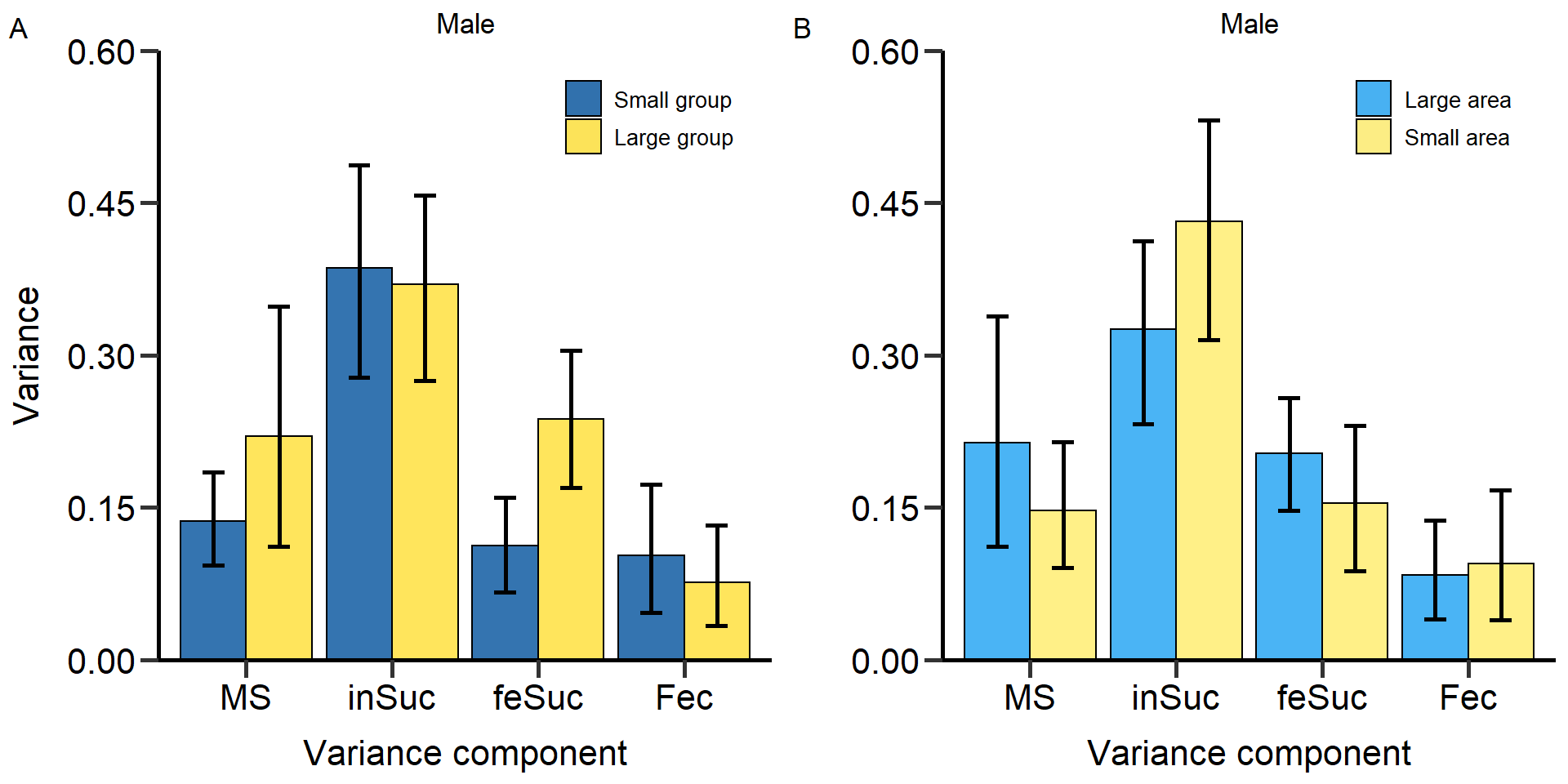 Figure 12: Variance decomposition for males into mating success,
insemination success, fertilization success and fecundity of the
partners. Means and 95% confidence intervals.
Figure 12: Variance decomposition for males into mating success,
insemination success, fertilization success and fecundity of the
partners. Means and 95% confidence intervals.
Treatement comparisons via permutation test for the variance decomposition of male reproductive success.
Table_VarianceDecomposition_TreatComp_round[c(1:8),c(2:7)] Treatment Variance_component Variance l95.CI u95.CI p-value
1 Group size MS -0.084 -0.218 0.033 0.091
2 Area MS 0.066 -0.059 0.208 0.171
3 Group size inSuc 0.016 -0.122 0.152 0.709
4 Area inSuc -0.106 -0.242 0.036 0.033
5 Group size feSuc -0.125 -0.206 -0.043 0.000
6 Area feSuc 0.048 -0.047 0.137 0.094
7 Group size Fec 0.026 -0.053 0.109 0.307
8 Area Fec -0.011 -0.096 0.067 0.663Variance decomposition for females
BarPlot_3<- ggplot(PhenVarBoot_Table_pop[9:12,], aes(x=Variance_component, y=Variance, fill=Treatment)) +
scale_y_continuous(limits = c(0, 2.7), breaks = seq(0,2.7,0.5), expand = c(0 ,0)) +
geom_hline(yintercept=0, linetype="solid", color = "black", size=1) +
geom_bar(stat="identity", color="black", position=position_dodge(), alpha=0.8) +
ylab('Variance') +xlab('Variance component') +ggtitle('Female')+labs(tag = "A")+
scale_x_discrete(breaks=waiver(),labels = c('MS','Fec'))+
theme(panel.border = element_blank(),
plot.title = element_text(hjust = 0.5),
panel.background = element_blank(),
panel.grid.major = element_blank(),
panel.grid.minor = element_blank(),
legend.position = c(0.8, 0.9),
plot.tag.position=c(0.01,0.98),
legend.title = element_blank(),
legend.text = element_text(colour="black", size=10),
axis.line.x = element_line(colour = "black", size = 1),
axis.line.y = element_line(colour = "black", size = 1),
axis.text.x = element_text(face="plain", color="black", size=16, angle=0),
axis.text.y = element_text(face="plain", color="black", size=16, angle=0),
axis.title.x = element_text(size=16,face="plain", margin = margin(r=0,10,0,0)),
axis.title.y = element_text(size=16,face="plain", margin = margin(r=10,0,0,0)),
axis.ticks = element_line(size = 1),
axis.ticks.length = unit(.3, "cm")) +
geom_errorbar(aes(ymin=l95.CI, ymax=u95.CI), width=.3,size=1, position=position_dodge(.9)) +
scale_fill_manual(values=c(colorESEB[1],colorESEB[2]),name = "Treatment", labels = c('Small group','Large group'))
BarPlot_4<- ggplot(PhenVarBoot_Table_area[9:12,], aes(x=Variance_component, y=Variance, fill=Treatment)) +
scale_y_continuous(limits = c(0, 2.7), breaks = seq(0,2.7,0.5), expand = c(0 ,0)) +
geom_hline(yintercept=0, linetype="solid", color = "black", size=1) +
geom_bar(stat="identity", color="black", position=position_dodge(), alpha=0.8) +
ylab('') +xlab('Variance component') +ggtitle('Female')+labs(tag = "B")+
scale_x_discrete(breaks=waiver(),labels = c('MS','Fec','cov\n(MS, Fec)'))+
theme(panel.border = element_blank(),
plot.title = element_text(hjust = 0.5),
panel.background = element_blank(),
panel.grid.major = element_blank(),
panel.grid.minor = element_blank(),
legend.position = c(0.8, 0.9),
plot.tag.position=c(0.01,0.98),
legend.title = element_blank(),
legend.text = element_text(colour="black", size=10),
axis.line.x = element_line(colour = "black", size = 1),
axis.line.y = element_line(colour = "black", size = 1),
axis.text.x = element_text(face="plain", color="black", size=16, angle=0),
axis.text.y = element_text(face="plain", color="black", size=16, angle=0),
axis.title.x = element_text(size=16,face="plain", margin = margin(r=0,10,0,0)),
axis.title.y = element_text(size=16,face="plain", margin = margin(r=10,0,0,0)),
axis.ticks = element_line(size = 1),
axis.ticks.length = unit(.3, "cm")) +
geom_errorbar(aes(ymin=l95.CI, ymax=u95.CI), width=.3,size=1, position=position_dodge(.9)) +
scale_fill_manual(values=c(colorESEB2[1],colorESEB2[2]),name = "Treatment", labels = c('Large area','Small area'))
grid.arrange(grobs = list(BarPlot_3,BarPlot_4), nrow = 1,ncol=2, widths=c(2.3, 2.3))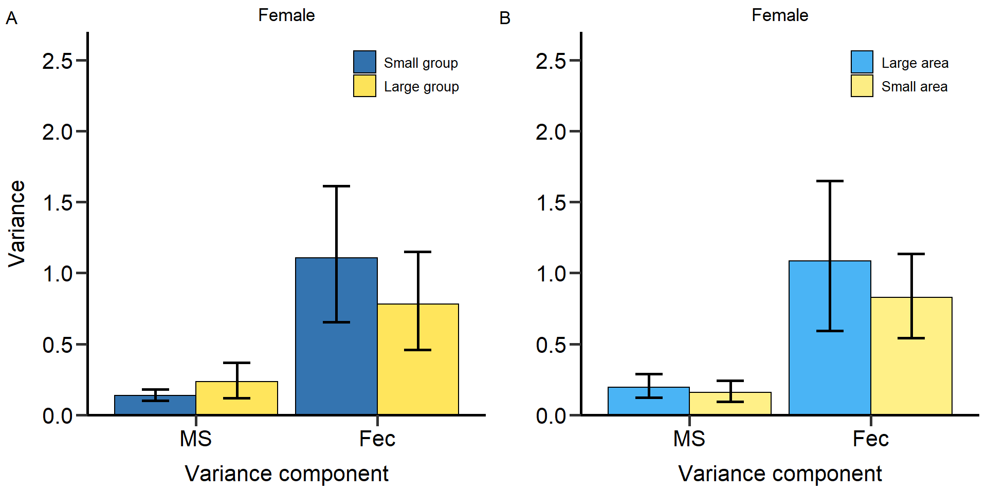 Figure 13: Variance decomposition for females into mating success,
fecundity and their covariance. Means and 95% confidence
intervals.
Figure 13: Variance decomposition for females into mating success,
fecundity and their covariance. Means and 95% confidence
intervals.
Treatement comparisons via permutation test for the
variance decomposition of female reproductive success.
Table_VarianceDecomposition_TreatComp_round[c(9:10),c(2:7)] Treatment Variance_component Variance l95.CI u95.CI p-value
9 Group size MS -0.098 -0.236 0.023 0.011
10 Area MS 0.036 -0.076 0.151 0.372Covariances for male variance decomposition
#Compute covariace matrices ####
# Large Area ####
#Covariance mMS x inSuc
x5=as.data.frame(cbind(DB_data_clean_Large_area_M_MS_n,DB_data_clean_Large_area_M_InSuc_n))
c <- function(d, i){
  d2 <- d[i,]
  return(cov(d2[1],d2[2],use='pairwise.complete.obs'))
}
Large_area_M_cov_mMS_inSuc_bootvar <- boot(x5, c, R=10000)


#Covariance mMS x feSuc
x6=as.data.frame(cbind(DB_data_clean_Large_area_M_MS_n,DB_data_clean_Large_area_M_feSuc_n))

Large_area_M_cov_mMS_feSuc_bootvar <- boot(x6, c, R=10000)


#Covariance mMS x pFec
x7=as.data.frame(cbind(DB_data_clean_Large_area_M_MS_n,DB_data_clean_Large_area_M_pFec_n))

Large_area_M_cov_mMS_pFec_bootvar <- boot(x7, c, R=10000)


#Covariance inSuc x feSuc
x8=as.data.frame(cbind(DB_data_clean_Large_area_M_InSuc_n,DB_data_clean_Large_area_M_feSuc_n))

Large_area_M_cov_inSuc_feSuc_bootvar <- boot(x8, c, R=10000)


#Covariance inSuc x pFec
x9=as.data.frame(cbind(DB_data_clean_Large_area_M_InSuc_n,DB_data_clean_Large_area_M_pFec_n))

Large_area_M_cov_inSuc_pFec_bootvar <- boot(x9, c, R=10000)


#Covariance feSuc x pFec
x10=as.data.frame(cbind(DB_data_clean_Large_area_M_feSuc_n,DB_data_clean_Large_area_M_pFec_n))

Large_area_M_cov_feSuc_pFec_bootvar <- boot(x10, c, R=10000)


#Covariance fMS x fFec
x13=as.data.frame(cbind(DB_data_clean_Large_area_F_fMS_n,DB_data_clean_Large_area_F_fFec_n))

Large_area_F_cov_fMS_fFec_bootvar <- boot(x13, c, R=10000)

rm("c")

#Write Table ####

PhenVarBoot_Table_Male_Large_area_cov_mMS_inSuc <- as.data.frame(cbind("Male", "cov_mMS_inSuc", "Large_area", mean(Large_area_M_cov_mMS_inSuc_bootvar$t), quantile(Large_area_M_cov_mMS_inSuc_bootvar$t,.025, names = FALSE), quantile(Large_area_M_cov_mMS_inSuc_bootvar$t,.975, names = FALSE)))
PhenVarBoot_Table_Male_Large_area_cov_mMS_feSuc <- as.data.frame(cbind("Male", "cov_mMS_feSuc", "Large_area", mean(Large_area_M_cov_mMS_feSuc_bootvar$t), quantile(Large_area_M_cov_mMS_feSuc_bootvar$t,.025, names = FALSE), quantile(Large_area_M_cov_mMS_feSuc_bootvar$t,.975, names = FALSE)))
PhenVarBoot_Table_Male_Large_area_cov_mMS_pFec <- as.data.frame(cbind("Male", "cov_mMS_pFec", "Large_area", mean(Large_area_M_cov_mMS_pFec_bootvar$t), quantile(Large_area_M_cov_mMS_pFec_bootvar$t,.025, names = FALSE), quantile(Large_area_M_cov_mMS_pFec_bootvar$t,.975, names = FALSE)))

PhenVarBoot_Table_Male_Large_area_cov_inSuc_feSuc <- as.data.frame(cbind("Male", "cov_inSuc_feSuc", "Large_area", mean(Large_area_M_cov_inSuc_feSuc_bootvar$t), quantile(Large_area_M_cov_inSuc_feSuc_bootvar$t,.025, names = FALSE), quantile(Large_area_M_cov_inSuc_feSuc_bootvar$t,.975, names = FALSE)))
PhenVarBoot_Table_Male_Large_area_cov_inSuc_pFec <- as.data.frame(cbind("Male", "cov_inSuc_pFec", "Large_area", mean(Large_area_M_cov_inSuc_pFec_bootvar$t), quantile(Large_area_M_cov_inSuc_pFec_bootvar$t,.025, names = FALSE), quantile(Large_area_M_cov_inSuc_pFec_bootvar$t,.975, names = FALSE)))

PhenVarBoot_Table_Male_Large_area_cov_feSuc_pFec <- as.data.frame(cbind("Male", "cov_feSuc_pFec", "Large_area", mean(Large_area_M_cov_feSuc_pFec_bootvar$t), quantile(Large_area_M_cov_feSuc_pFec_bootvar$t,.025, names = FALSE), quantile(Large_area_M_cov_feSuc_pFec_bootvar$t,.975, names = FALSE)))

PhenVarBoot_Table_Female_Large_area_cov_fMS_fFec <- as.data.frame(cbind("Female", "cov_fMS_fFec", "Large_area", mean(Large_area_F_cov_fMS_fFec_bootvar$t), quantile(Large_area_F_cov_fMS_fFec_bootvar$t,.025, names = FALSE), quantile(Large_area_F_cov_fMS_fFec_bootvar$t,.975, names = FALSE)))


PhenVarBoot_Cov_Table_Large_area <- as.data.frame(as.matrix(rbind(PhenVarBoot_Table_Male_Large_area_cov_mMS_inSuc,PhenVarBoot_Table_Male_Large_area_cov_mMS_feSuc,
                                                            PhenVarBoot_Table_Male_Large_area_cov_mMS_pFec,PhenVarBoot_Table_Male_Large_area_cov_inSuc_feSuc,
                                                            PhenVarBoot_Table_Male_Large_area_cov_inSuc_pFec,PhenVarBoot_Table_Male_Large_area_cov_feSuc_pFec,
                                                            PhenVarBoot_Table_Female_Large_area_cov_fMS_fFec)),digits=3)

is.table(PhenVarBoot_Cov_Table_Large_area)
colnames(PhenVarBoot_Cov_Table_Large_area)[1] <- "Sex"
colnames(PhenVarBoot_Cov_Table_Large_area)[2] <- "Trait"
colnames(PhenVarBoot_Cov_Table_Large_area)[3] <- "Density"
colnames(PhenVarBoot_Cov_Table_Large_area)[4] <- "Variance"
colnames(PhenVarBoot_Cov_Table_Large_area)[5] <- "l95.CI"
colnames(PhenVarBoot_Cov_Table_Large_area)[6] <- "u95.CI"
PhenVarBoot_Cov_Table_Large_area[,4]=as.numeric(PhenVarBoot_Cov_Table_Large_area[,4])
PhenVarBoot_Cov_Table_Large_area[,5]=as.numeric(PhenVarBoot_Cov_Table_Large_area[,5])
PhenVarBoot_Cov_Table_Large_area[,6]=as.numeric(PhenVarBoot_Cov_Table_Large_area[,6])

PhenVarBoot_Cov_Table_Large_area_round=cbind(PhenVarBoot_Cov_Table_Large_area[,1:3],round(PhenVarBoot_Cov_Table_Large_area[,4:6],digit=3))

# Small Area ####
#Covariance mMS x inSuc
x5=as.data.frame(cbind(DB_data_clean_Small_area_M_MS_n,DB_data_clean_Small_area_M_InSuc_n))
c <- function(d, i){
  d2 <- d[i,]
  return(cov(d2[1],d2[2],use='pairwise.complete.obs'))
}
Small_area_M_cov_mMS_inSuc_bootvar <- boot(x5, c, R=10000)


#Covariance mMS x feSuc
x6=as.data.frame(cbind(DB_data_clean_Small_area_M_MS_n,DB_data_clean_Small_area_M_feSuc_n))

Small_area_M_cov_mMS_feSuc_bootvar <- boot(x6, c, R=10000)


#Covariance mMS x pFec
x7=as.data.frame(cbind(DB_data_clean_Small_area_M_MS_n,DB_data_clean_Small_area_M_pFec_n))

Small_area_M_cov_mMS_pFec_bootvar <- boot(x7, c, R=10000)


#Covariance inSuc x feSuc
x8=as.data.frame(cbind(DB_data_clean_Small_area_M_InSuc_n,DB_data_clean_Small_area_M_feSuc_n))

Small_area_M_cov_inSuc_feSuc_bootvar <- boot(x8, c, R=10000)


#Covariance inSuc x pFec
x9=as.data.frame(cbind(DB_data_clean_Small_area_M_InSuc_n,DB_data_clean_Small_area_M_pFec_n))

Small_area_M_cov_inSuc_pFec_bootvar <- boot(x9, c, R=10000)

#Covariance feSuc x pFec
x10=as.data.frame(cbind(DB_data_clean_Small_area_M_feSuc_n,DB_data_clean_Small_area_M_pFec_n))

Small_area_M_cov_feSuc_pFec_bootvar <- boot(x10, c, R=10000)


#Covariance fMS x fFec
x13=as.data.frame(cbind(DB_data_clean_Small_area_F_fMS_n,DB_data_clean_Small_area_F_fFec_n))

Small_area_F_cov_fMS_fFec_bootvar <- boot(x13, c, R=10000)

rm("c")

#Write Table ####

PhenVarBoot_Table_Male_Small_area_cov_mMS_inSuc <- as.data.frame(cbind("Male", "cov_mMS_inSuc", "Small_area", mean(Small_area_M_cov_mMS_inSuc_bootvar$t), quantile(Small_area_M_cov_mMS_inSuc_bootvar$t,.025, names = FALSE), quantile(Small_area_M_cov_mMS_inSuc_bootvar$t,.975, names = FALSE)))
PhenVarBoot_Table_Male_Small_area_cov_mMS_feSuc <- as.data.frame(cbind("Male", "cov_mMS_feSuc", "Small_area", mean(Small_area_M_cov_mMS_feSuc_bootvar$t), quantile(Small_area_M_cov_mMS_feSuc_bootvar$t,.025, names = FALSE), quantile(Small_area_M_cov_mMS_feSuc_bootvar$t,.975, names = FALSE)))
PhenVarBoot_Table_Male_Small_area_cov_mMS_pFec <- as.data.frame(cbind("Male", "cov_mMS_pFec", "Small_area", mean(Small_area_M_cov_mMS_pFec_bootvar$t), quantile(Small_area_M_cov_mMS_pFec_bootvar$t,.025, names = FALSE), quantile(Small_area_M_cov_mMS_pFec_bootvar$t,.975, names = FALSE)))

PhenVarBoot_Table_Male_Small_area_cov_inSuc_feSuc <- as.data.frame(cbind("Male", "cov_inSuc_feSuc", "Small_area", mean(Small_area_M_cov_inSuc_feSuc_bootvar$t), quantile(Small_area_M_cov_inSuc_feSuc_bootvar$t,.025, names = FALSE), quantile(Small_area_M_cov_inSuc_feSuc_bootvar$t,.975, names = FALSE)))
PhenVarBoot_Table_Male_Small_area_cov_inSuc_pFec <- as.data.frame(cbind("Male", "cov_inSuc_pFec", "Small_area", mean(Small_area_M_cov_inSuc_pFec_bootvar$t), quantile(Small_area_M_cov_inSuc_pFec_bootvar$t,.025, names = FALSE), quantile(Small_area_M_cov_inSuc_pFec_bootvar$t,.975, names = FALSE)))

PhenVarBoot_Table_Male_Small_area_cov_feSuc_pFec <- as.data.frame(cbind("Male", "cov_feSuc_pFec", "Small_area", mean(Small_area_M_cov_feSuc_pFec_bootvar$t), quantile(Small_area_M_cov_feSuc_pFec_bootvar$t,.025, names = FALSE), quantile(Small_area_M_cov_feSuc_pFec_bootvar$t,.975, names = FALSE)))

PhenVarBoot_Table_Female_Small_area_cov_fMS_fFec <- as.data.frame(cbind("Female", "cov_fMS_fFec", "Small_area", mean(Small_area_F_cov_fMS_fFec_bootvar$t), quantile(Small_area_F_cov_fMS_fFec_bootvar$t,.025, names = FALSE), quantile(Small_area_F_cov_fMS_fFec_bootvar$t,.975, names = FALSE)))


PhenVarBoot_Cov_Table_Small_area <- as.data.frame(as.matrix(rbind(PhenVarBoot_Table_Male_Small_area_cov_mMS_inSuc,PhenVarBoot_Table_Male_Small_area_cov_mMS_feSuc,
                                                            PhenVarBoot_Table_Male_Small_area_cov_mMS_pFec,PhenVarBoot_Table_Male_Small_area_cov_inSuc_feSuc,
                                                            PhenVarBoot_Table_Male_Small_area_cov_inSuc_pFec,PhenVarBoot_Table_Male_Small_area_cov_feSuc_pFec,
                                                            PhenVarBoot_Table_Female_Small_area_cov_fMS_fFec)),digits=3)

is.table(PhenVarBoot_Cov_Table_Small_area)
colnames(PhenVarBoot_Cov_Table_Small_area)[1] <- "Sex"
colnames(PhenVarBoot_Cov_Table_Small_area)[2] <- "Trait"
colnames(PhenVarBoot_Cov_Table_Small_area)[3] <- "Density"
colnames(PhenVarBoot_Cov_Table_Small_area)[4] <- "Variance"
colnames(PhenVarBoot_Cov_Table_Small_area)[5] <- "l95.CI"
colnames(PhenVarBoot_Cov_Table_Small_area)[6] <- "u95.CI"
PhenVarBoot_Cov_Table_Small_area[,4]=as.numeric(PhenVarBoot_Cov_Table_Small_area[,4])
PhenVarBoot_Cov_Table_Small_area[,5]=as.numeric(PhenVarBoot_Cov_Table_Small_area[,5])
PhenVarBoot_Cov_Table_Small_area[,6]=as.numeric(PhenVarBoot_Cov_Table_Small_area[,6])

PhenVarBoot_Cov_Table_Small_area_round=cbind(PhenVarBoot_Cov_Table_Small_area[,1:3],round(PhenVarBoot_Cov_Table_Small_area[,4:6],digit=3))

# Small group ####
#Covariance mMS x inSuc
x5=as.data.frame(cbind(DB_data_clean_Small_pop_M_MS_n,DB_data_clean_Small_pop_M_InSuc_n))
c <- function(d, i){
  d2 <- d[i,]
  return(cov(d2[1],d2[2],use='pairwise.complete.obs'))
}
Small_pop_M_cov_mMS_inSuc_bootvar <- boot(x5, c, R=10000)


#Covariance mMS x feSuc
x6=as.data.frame(cbind(DB_data_clean_Small_pop_M_MS_n,DB_data_clean_Small_pop_M_feSuc_n))

Small_pop_M_cov_mMS_feSuc_bootvar <- boot(x6, c, R=10000)


#Covariance mMS x pFec
x7=as.data.frame(cbind(DB_data_clean_Small_pop_M_MS_n,DB_data_clean_Small_pop_M_pFec_n))

Small_pop_M_cov_mMS_pFec_bootvar <- boot(x7, c, R=10000)


#Covariance inSuc x feSuc
x8=as.data.frame(cbind(DB_data_clean_Small_pop_M_InSuc_n,DB_data_clean_Small_pop_M_feSuc_n))

Small_pop_M_cov_inSuc_feSuc_bootvar <- boot(x8, c, R=10000)

#Covariance inSuc x pFec
x9=as.data.frame(cbind(DB_data_clean_Small_pop_M_InSuc_n,DB_data_clean_Small_pop_M_pFec_n))

Small_pop_M_cov_inSuc_pFec_bootvar <- boot(x9, c, R=10000)


#Covariance feSuc x pFec
x10=as.data.frame(cbind(DB_data_clean_Small_pop_M_feSuc_n,DB_data_clean_Small_pop_M_pFec_n))

Small_pop_M_cov_feSuc_pFec_bootvar <- boot(x10, c, R=10000)


#Covariance fMS x fFec
x13=as.data.frame(cbind(DB_data_clean_Small_pop_F_fMS_n,DB_data_clean_Small_pop_F_fFec_n))

Small_pop_F_cov_fMS_fFec_bootvar <- boot(x13, c, R=10000)

rm("c")

#Write Table ####

PhenVarBoot_Table_Male_Small_pop_cov_mMS_inSuc <- as.data.frame(cbind("Male", "cov_mMS_inSuc", "Small_pop", mean(Small_pop_M_cov_mMS_inSuc_bootvar$t), quantile(Small_pop_M_cov_mMS_inSuc_bootvar$t,.025, names = FALSE), quantile(Small_pop_M_cov_mMS_inSuc_bootvar$t,.975, names = FALSE)))
PhenVarBoot_Table_Male_Small_pop_cov_mMS_feSuc <- as.data.frame(cbind("Male", "cov_mMS_feSuc", "Small_pop", mean(Small_pop_M_cov_mMS_feSuc_bootvar$t), quantile(Small_pop_M_cov_mMS_feSuc_bootvar$t,.025, names = FALSE), quantile(Small_pop_M_cov_mMS_feSuc_bootvar$t,.975, names = FALSE)))
PhenVarBoot_Table_Male_Small_pop_cov_mMS_pFec <- as.data.frame(cbind("Male", "cov_mMS_pFec", "Small_pop", mean(Small_pop_M_cov_mMS_pFec_bootvar$t), quantile(Small_pop_M_cov_mMS_pFec_bootvar$t,.025, names = FALSE), quantile(Small_pop_M_cov_mMS_pFec_bootvar$t,.975, names = FALSE)))

PhenVarBoot_Table_Male_Small_pop_cov_inSuc_feSuc <- as.data.frame(cbind("Male", "cov_inSuc_feSuc", "Small_pop", mean(Small_pop_M_cov_inSuc_feSuc_bootvar$t), quantile(Small_pop_M_cov_inSuc_feSuc_bootvar$t,.025, names = FALSE), quantile(Small_pop_M_cov_inSuc_feSuc_bootvar$t,.975, names = FALSE)))
PhenVarBoot_Table_Male_Small_pop_cov_inSuc_pFec <- as.data.frame(cbind("Male", "cov_inSuc_pFec", "Small_pop", mean(Small_pop_M_cov_inSuc_pFec_bootvar$t), quantile(Small_pop_M_cov_inSuc_pFec_bootvar$t,.025, names = FALSE), quantile(Small_pop_M_cov_inSuc_pFec_bootvar$t,.975, names = FALSE)))

PhenVarBoot_Table_Male_Small_pop_cov_feSuc_pFec <- as.data.frame(cbind("Male", "cov_feSuc_pFec", "Small_pop", mean(Small_pop_M_cov_feSuc_pFec_bootvar$t), quantile(Small_pop_M_cov_feSuc_pFec_bootvar$t,.025, names = FALSE), quantile(Small_pop_M_cov_feSuc_pFec_bootvar$t,.975, names = FALSE)))

PhenVarBoot_Table_Female_Small_pop_cov_fMS_fFec <- as.data.frame(cbind("Female", "cov_fMS_fFec", "Small_pop", mean(Small_pop_F_cov_fMS_fFec_bootvar$t), quantile(Small_pop_F_cov_fMS_fFec_bootvar$t,.025, names = FALSE), quantile(Small_pop_F_cov_fMS_fFec_bootvar$t,.975, names = FALSE)))


PhenVarBoot_Cov_Table_Small_pop <- as.data.frame(as.matrix(rbind(PhenVarBoot_Table_Male_Small_pop_cov_mMS_inSuc,PhenVarBoot_Table_Male_Small_pop_cov_mMS_feSuc,
                                                            PhenVarBoot_Table_Male_Small_pop_cov_mMS_pFec,PhenVarBoot_Table_Male_Small_pop_cov_inSuc_feSuc,
                                                            PhenVarBoot_Table_Male_Small_pop_cov_inSuc_pFec,PhenVarBoot_Table_Male_Small_pop_cov_feSuc_pFec,
                                                            PhenVarBoot_Table_Female_Small_pop_cov_fMS_fFec)),digits=3)

is.table(PhenVarBoot_Cov_Table_Small_pop)
colnames(PhenVarBoot_Cov_Table_Small_pop)[1] <- "Sex"
colnames(PhenVarBoot_Cov_Table_Small_pop)[2] <- "Trait"
colnames(PhenVarBoot_Cov_Table_Small_pop)[3] <- "Density"
colnames(PhenVarBoot_Cov_Table_Small_pop)[4] <- "Variance"
colnames(PhenVarBoot_Cov_Table_Small_pop)[5] <- "l95.CI"
colnames(PhenVarBoot_Cov_Table_Small_pop)[6] <- "u95.CI"
PhenVarBoot_Cov_Table_Small_pop[,4]=as.numeric(PhenVarBoot_Cov_Table_Small_pop[,4])
PhenVarBoot_Cov_Table_Small_pop[,5]=as.numeric(PhenVarBoot_Cov_Table_Small_pop[,5])
PhenVarBoot_Cov_Table_Small_pop[,6]=as.numeric(PhenVarBoot_Cov_Table_Small_pop[,6])

PhenVarBoot_Cov_Table_Small_pop_round=cbind(PhenVarBoot_Cov_Table_Small_pop[,1:3],round(PhenVarBoot_Cov_Table_Small_pop[,4:6],digit=3))

# Large group ####
#Covariance mMS x inSuc
x5=as.data.frame(cbind(DB_data_clean_Large_pop_M_MS_n,DB_data_clean_Large_pop_M_InSuc_n))
c <- function(d, i){
  d2 <- d[i,]
  return(cov(d2[1],d2[2],use='pairwise.complete.obs'))
}
Large_pop_M_cov_mMS_inSuc_bootvar <- boot(x5, c, R=10000)


#Covariance mMS x feSuc
x6=as.data.frame(cbind(DB_data_clean_Large_pop_M_MS_n,DB_data_clean_Large_pop_M_feSuc_n))

Large_pop_M_cov_mMS_feSuc_bootvar <- boot(x6, c, R=10000)


#Covariance mMS x pFec
x7=as.data.frame(cbind(DB_data_clean_Large_pop_M_MS_n,DB_data_clean_Large_pop_M_pFec_n))

Large_pop_M_cov_mMS_pFec_bootvar <- boot(x7, c, R=10000)


#Covariance inSuc x feSuc
x8=as.data.frame(cbind(DB_data_clean_Large_pop_M_InSuc_n,DB_data_clean_Large_pop_M_feSuc_n))

Large_pop_M_cov_inSuc_feSuc_bootvar <- boot(x8, c, R=10000)


#Covariance inSuc x pFec
x9=as.data.frame(cbind(DB_data_clean_Large_pop_M_InSuc_n,DB_data_clean_Large_pop_M_pFec_n))

Large_pop_M_cov_inSuc_pFec_bootvar <- boot(x9, c, R=10000)


#Covariance feSuc x pFec
x10=as.data.frame(cbind(DB_data_clean_Large_pop_M_feSuc_n,DB_data_clean_Large_pop_M_pFec_n))

Large_pop_M_cov_feSuc_pFec_bootvar <- boot(x10, c, R=10000)


#Covariance fMS x fFec
x13=as.data.frame(cbind(DB_data_clean_Large_pop_F_fMS_n,DB_data_clean_Large_pop_F_fFec_n))

Large_pop_F_cov_fMS_fFec_bootvar <- boot(x13, c, R=10000)

rm("c")

#Write Table ####

PhenVarBoot_Table_Male_Large_pop_cov_mMS_inSuc <- as.data.frame(cbind("Male", "cov_mMS_inSuc", "Large_pop", mean(Large_pop_M_cov_mMS_inSuc_bootvar$t), quantile(Large_pop_M_cov_mMS_inSuc_bootvar$t,.025, names = FALSE), quantile(Large_pop_M_cov_mMS_inSuc_bootvar$t,.975, names = FALSE)))
PhenVarBoot_Table_Male_Large_pop_cov_mMS_feSuc <- as.data.frame(cbind("Male", "cov_mMS_feSuc", "Large_pop", mean(Large_pop_M_cov_mMS_feSuc_bootvar$t), quantile(Large_pop_M_cov_mMS_feSuc_bootvar$t,.025, names = FALSE), quantile(Large_pop_M_cov_mMS_feSuc_bootvar$t,.975, names = FALSE)))
PhenVarBoot_Table_Male_Large_pop_cov_mMS_pFec <- as.data.frame(cbind("Male", "cov_mMS_pFec", "Large_pop", mean(Large_pop_M_cov_mMS_pFec_bootvar$t), quantile(Large_pop_M_cov_mMS_pFec_bootvar$t,.025, names = FALSE), quantile(Large_pop_M_cov_mMS_pFec_bootvar$t,.975, names = FALSE)))

PhenVarBoot_Table_Male_Large_pop_cov_inSuc_feSuc <- as.data.frame(cbind("Male", "cov_inSuc_feSuc", "Large_pop", mean(Large_pop_M_cov_inSuc_feSuc_bootvar$t), quantile(Large_pop_M_cov_inSuc_feSuc_bootvar$t,.025, names = FALSE), quantile(Large_pop_M_cov_inSuc_feSuc_bootvar$t,.975, names = FALSE)))
PhenVarBoot_Table_Male_Large_pop_cov_inSuc_pFec <- as.data.frame(cbind("Male", "cov_inSuc_pFec", "Large_pop", mean(Large_pop_M_cov_inSuc_pFec_bootvar$t), quantile(Large_pop_M_cov_inSuc_pFec_bootvar$t,.025, names = FALSE), quantile(Large_pop_M_cov_inSuc_pFec_bootvar$t,.975, names = FALSE)))

PhenVarBoot_Table_Male_Large_pop_cov_feSuc_pFec <- as.data.frame(cbind("Male", "cov_feSuc_pFec", "Large_pop", mean(Large_pop_M_cov_feSuc_pFec_bootvar$t), quantile(Large_pop_M_cov_feSuc_pFec_bootvar$t,.025, names = FALSE), quantile(Large_pop_M_cov_feSuc_pFec_bootvar$t,.975, names = FALSE)))

PhenVarBoot_Table_Female_Large_pop_cov_fMS_fFec <- as.data.frame(cbind("Female", "cov_fMS_fFec", "Large_pop", mean(Large_pop_F_cov_fMS_fFec_bootvar$t), quantile(Large_pop_F_cov_fMS_fFec_bootvar$t,.025, names = FALSE), quantile(Large_pop_F_cov_fMS_fFec_bootvar$t,.975, names = FALSE)))


PhenVarBoot_Cov_Table_Large_pop <- as.data.frame(as.matrix(rbind(PhenVarBoot_Table_Male_Large_pop_cov_mMS_inSuc,PhenVarBoot_Table_Male_Large_pop_cov_mMS_feSuc,
                                                            PhenVarBoot_Table_Male_Large_pop_cov_mMS_pFec,PhenVarBoot_Table_Male_Large_pop_cov_inSuc_feSuc,
                                                            PhenVarBoot_Table_Male_Large_pop_cov_inSuc_pFec,PhenVarBoot_Table_Male_Large_pop_cov_feSuc_pFec,
                                                            PhenVarBoot_Table_Female_Large_pop_cov_fMS_fFec)),digits=3)

is.table(PhenVarBoot_Cov_Table_Large_pop)
colnames(PhenVarBoot_Cov_Table_Large_pop)[1] <- "Sex"
colnames(PhenVarBoot_Cov_Table_Large_pop)[2] <- "Trait"
colnames(PhenVarBoot_Cov_Table_Large_pop)[3] <- "Density"
colnames(PhenVarBoot_Cov_Table_Large_pop)[4] <- "Variance"
colnames(PhenVarBoot_Cov_Table_Large_pop)[5] <- "l95.CI"
colnames(PhenVarBoot_Cov_Table_Large_pop)[6] <- "u95.CI"
PhenVarBoot_Cov_Table_Large_pop[,4]=as.numeric(PhenVarBoot_Cov_Table_Large_pop[,4])
PhenVarBoot_Cov_Table_Large_pop[,5]=as.numeric(PhenVarBoot_Cov_Table_Large_pop[,5])
PhenVarBoot_Cov_Table_Large_pop[,6]=as.numeric(PhenVarBoot_Cov_Table_Large_pop[,6])

PhenVarBoot_Cov_Table_Large_pop_round=cbind(PhenVarBoot_Cov_Table_Large_pop[,1:3],round(PhenVarBoot_Cov_Table_Large_pop[,4:6],digit=3))

#Figure ####
PhenVarBoot_Table_plot_cov <- as.data.frame(as.matrix(rbind( PhenVarBoot_Table_Male_Small_pop_cov_mMS_inSuc,PhenVarBoot_Table_Male_Large_pop_cov_mMS_inSuc,
                                                             PhenVarBoot_Table_Male_Large_area_cov_mMS_inSuc,PhenVarBoot_Table_Male_Small_area_cov_mMS_inSuc,
                                                             PhenVarBoot_Table_Male_Small_pop_cov_mMS_feSuc,PhenVarBoot_Table_Male_Large_pop_cov_mMS_feSuc,
                                                             PhenVarBoot_Table_Male_Large_area_cov_mMS_feSuc,PhenVarBoot_Table_Male_Small_area_cov_mMS_feSuc,
                                                             PhenVarBoot_Table_Male_Small_pop_cov_mMS_pFec,PhenVarBoot_Table_Male_Large_pop_cov_mMS_pFec,
                                                             PhenVarBoot_Table_Male_Large_area_cov_mMS_pFec,PhenVarBoot_Table_Male_Small_area_cov_mMS_pFec,
                                                             PhenVarBoot_Table_Male_Small_pop_cov_inSuc_feSuc,PhenVarBoot_Table_Male_Large_pop_cov_inSuc_feSuc,
                                                             PhenVarBoot_Table_Male_Large_area_cov_inSuc_feSuc,PhenVarBoot_Table_Male_Small_area_cov_inSuc_feSuc,
                                                              PhenVarBoot_Table_Male_Small_pop_cov_inSuc_pFec,PhenVarBoot_Table_Male_Large_pop_cov_inSuc_pFec,
                                                             PhenVarBoot_Table_Male_Large_area_cov_inSuc_pFec,PhenVarBoot_Table_Male_Small_area_cov_inSuc_pFec,
                                                             PhenVarBoot_Table_Male_Small_pop_cov_feSuc_pFec,PhenVarBoot_Table_Male_Large_pop_cov_feSuc_pFec,
                                                             PhenVarBoot_Table_Male_Large_area_cov_feSuc_pFec,PhenVarBoot_Table_Male_Small_area_cov_feSuc_pFec,
                                                            PhenVarBoot_Table_Female_Small_pop_cov_fMS_fFec,PhenVarBoot_Table_Female_Large_pop_cov_fMS_fFec,
                                                             PhenVarBoot_Table_Female_Large_area_cov_fMS_fFec,PhenVarBoot_Table_Female_Small_area_cov_fMS_fFec
                                                             )))

is.table(PhenVarBoot_Table_plot_cov)
colnames(PhenVarBoot_Table_plot_cov)[1] <- "Sex"
colnames(PhenVarBoot_Table_plot_cov)[2] <- "Variance_component"
colnames(PhenVarBoot_Table_plot_cov)[3] <- "Treatment"
colnames(PhenVarBoot_Table_plot_cov)[4] <- "Variance"
colnames(PhenVarBoot_Table_plot_cov)[5] <- "l95.CI"
colnames(PhenVarBoot_Table_plot_cov)[6] <- "u95.CI"
PhenVarBoot_Table_plot_cov[,4]=as.numeric(PhenVarBoot_Table_plot_cov[,4])
PhenVarBoot_Table_plot_cov[,5]=as.numeric(PhenVarBoot_Table_plot_cov[,5])
PhenVarBoot_Table_plot_cov[,6]=as.numeric(PhenVarBoot_Table_plot_cov[,6])

PhenVarBoot_Table_plot_cov_round=cbind(PhenVarBoot_Table_plot_cov[,1:3],round(PhenVarBoot_Table_plot_cov[,4:6],digit=3))

PhenVarBoot_Table_plot_cov$Treatment<- factor(PhenVarBoot_Table_plot_cov$Treatment, levels=c("Small_pop",'Large_pop','Large_area','Small_area'))
PhenVarBoot_Table_plot_cov$Variance_component <- factor(PhenVarBoot_Table_plot_cov$Variance_component, levels=c("cov_mMS_inSuc",'cov_mMS_feSuc','cov_mMS_pFec','cov_inSuc_feSuc','cov_inSuc_pFec','cov_feSuc_pFec','cov_fMS_fFec'))
PhenVarBoot_Table_plot_cov_area=PhenVarBoot_Table_plot_cov[PhenVarBoot_Table_plot_cov$Treatment!='Large_pop',]
PhenVarBoot_Table_plot_cov_area=PhenVarBoot_Table_plot_cov_area[PhenVarBoot_Table_plot_cov_area$Treatment!='Small_pop',]
PhenVarBoot_Table_plot_cov_pop=PhenVarBoot_Table_plot_cov[PhenVarBoot_Table_plot_cov$Treatment!='Large_area',]
PhenVarBoot_Table_plot_cov_pop=PhenVarBoot_Table_plot_cov_pop[PhenVarBoot_Table_plot_cov_pop$Treatment!='Small_area',]
Figure: Covariances of variance decomposition for females
BarPlot_5<- ggplot(PhenVarBoot_Table_plot_cov_pop[1:12,], aes(x=Variance_component, y=Variance, fill=Treatment)) +
scale_y_continuous(limits = c(-0.25, 0.2), breaks = seq(-0.25,0.2,0.1), expand = c(0 ,0)) +
geom_hline(yintercept=0, linetype="solid", color = "black", size=1) +
geom_bar(stat="identity", color="black", position=position_dodge(), alpha=0.8) +
geom_errorbar(aes(ymin=l95.CI, ymax=u95.CI), width=.3,size=1, position=position_dodge(.9)) +
ylab('Variance') +xlab('Variance component') +ggtitle('Male')+labs(tag = "A")+
scale_x_discrete(breaks=waiver(),labels = c('cov\n(MS, inSuc)','cov\n(MS, feSuc)','cov\n(MS, Fec)','cov\n(inSuc, feSuc)','cov\n(inSuc,Fec)','cov\n(feSuc, Fec)'))+
theme(panel.border = element_blank(),
plot.title = element_text(hjust = 0.5),
panel.background = element_blank(),
panel.grid.major = element_blank(),
panel.grid.minor = element_blank(),
plot.tag.position=c(0.01,0.98),
legend.position = c(0.8, 0.9),
legend.title = element_blank(),
legend.text = element_text(colour="black", size=10),
axis.line.x = element_line(colour = "black", size = 1),
axis.line.y = element_line(colour = "black", size = 1),
axis.text.x = element_text(face="plain", color="black", size=16, angle=0),
axis.text.y = element_text(face="plain", color="black", size=16, angle=0),
axis.title.x = element_text(size=16,face="plain", margin = margin(r=0,10,0,0)),
axis.title.y = element_text(size=16,face="plain", margin = margin(r=10,0,0,0)),
axis.ticks = element_line(size = 1),
axis.ticks.length = unit(.3, "cm"))+
scale_fill_manual(values=c(colorESEB[1],colorESEB[2]),name = "Treatment", labels = c('Small group','Large group'))
BarPlot_6<-ggplot(PhenVarBoot_Table_plot_cov_area[1:12,], aes(x=Variance_component, y=Variance, fill=Treatment)) +
scale_y_continuous(limits = c(-0.25, 0.2), breaks = seq(-0.25,0.2,0.1), expand = c(0 ,0)) +
geom_hline(yintercept=0, linetype="solid", color = "black", size=1) +
geom_bar(stat="identity", color="black", position=position_dodge(), alpha=0.8) +
geom_errorbar(aes(ymin=l95.CI, ymax=u95.CI), width=.3,size=1, position=position_dodge(.9)) +
ylab('') +xlab('Variance component') +ggtitle('Male')+labs(tag = "B")+
scale_x_discrete(breaks=waiver(),labels = c('cov\n(MS, inSuc)','cov\n(MS, feSuc)','cov\n(MS, Fec)','cov\n(inSuc, feSuc)','cov\n(inSuc,Fec)','cov\n(feSuc, Fec)'))+
scale_fill_manual(values=c(colorESEB2[1],colorESEB2[2]),name = "Treatment", labels = c('Large area','Small area'))+
theme(panel.border = element_blank(),
plot.title = element_text(hjust = 0.5),
panel.background = element_blank(),
panel.grid.major = element_blank(),
panel.grid.minor = element_blank(),
legend.position = c(0.8, 0.9),
plot.tag.position=c(0.01,0.98),
legend.title = element_blank(),
legend.text = element_text(colour="black", size=10),
axis.line.x = element_line(colour = "black", size = 1),
axis.line.y = element_line(colour = "black", size = 1),
axis.text.x = element_text(face="plain", color="black", size=16, angle=0),
axis.text.y = element_text(face="plain", color="black", size=16, angle=0),
axis.title.x = element_text(size=16,face="plain", margin = margin(r=0,10,0,0)),
axis.title.y = element_text(size=16,face="plain", margin = margin(r=10,0,0,0)),
axis.ticks = element_line(size = 1),
axis.ticks.length = unit(.3, "cm"))
grid.arrange(grobs = list(BarPlot_5,BarPlot_6), nrow = 1,ncol=2, widths=c(2.3, 2.3))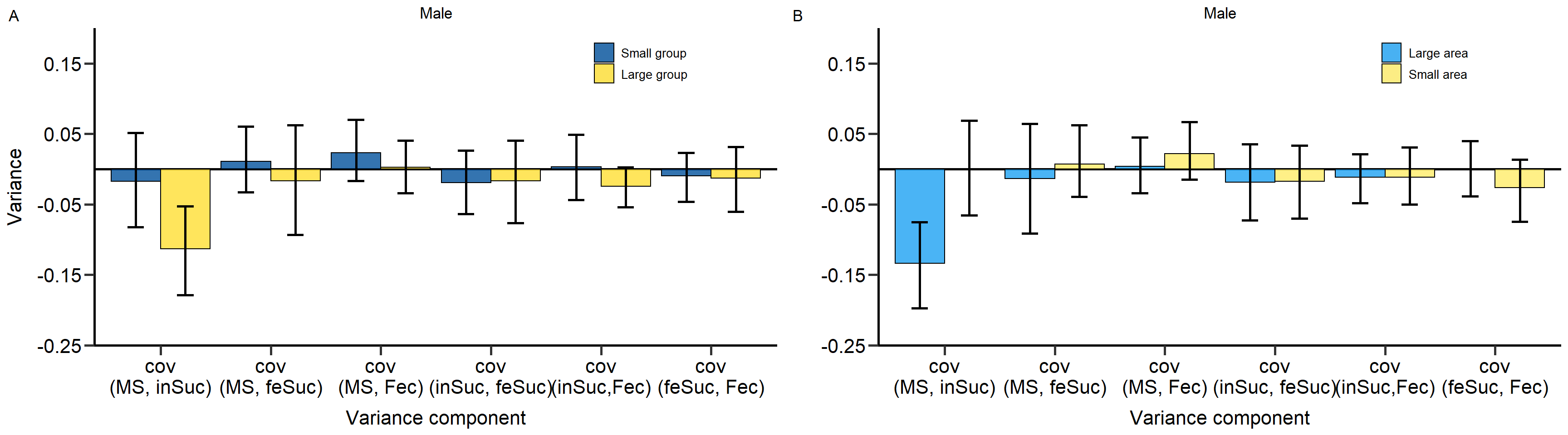 Figure 14: Covariance components for variance decomposition in males
into mating success, insemination success, fertilization success and
fecundity of the partners. Means and 95% confidence
intervals.
Figure 14: Covariance components for variance decomposition in males
into mating success, insemination success, fertilization success and
fecundity of the partners. Means and 95% confidence
intervals.
sessionInfo()R version 4.2.0 (2022-04-22 ucrt)
Platform: x86_64-w64-mingw32/x64 (64-bit)
Running under: Windows 10 x64 (build 19043)
Matrix products: default
locale:
[1] LC_COLLATE=German_Germany.utf8 LC_CTYPE=German_Germany.utf8
[3] LC_MONETARY=German_Germany.utf8 LC_NUMERIC=C
[5] LC_TIME=German_Germany.utf8
attached base packages:
[1] grid stats graphics grDevices utils datasets methods
[8] base
other attached packages:
[1] ICC_2.4.0 tidyr_1.2.0 data.table_1.14.2 boot_1.3-28
[5] RColorBrewer_1.1-3 car_3.1-0 carData_3.0-5 gridGraphics_0.5-1
[9] cowplot_1.1.1 EnvStats_2.7.0 dplyr_1.0.9 readr_2.1.2
[13] lmerTest_3.1-3 lme4_1.1-30 Matrix_1.4-1 gridExtra_2.3
[17] ggplot2_3.3.6 ggeffects_1.1.3 workflowr_1.7.0
loaded via a namespace (and not attached):
[1] httr_1.4.3 sass_0.4.2 bit64_4.0.5
[4] vroom_1.5.7 jsonlite_1.8.0 splines_4.2.0
[7] bslib_0.4.0 getPass_0.2-2 highr_0.9
[10] yaml_2.3.5 numDeriv_2016.8-1.1 pillar_1.8.0
[13] lattice_0.20-45 glue_1.6.2 digest_0.6.29
[16] promises_1.2.0.1 minqa_1.2.4 colorspace_2.0-3
[19] htmltools_0.5.3 httpuv_1.6.5 pkgconfig_2.0.3
[22] purrr_0.3.4 scales_1.2.0 processx_3.7.0
[25] whisker_0.4 later_1.3.0 tzdb_0.3.0
[28] git2r_0.30.1 tibble_3.1.7 mgcv_1.8-40
[31] farver_2.1.1 generics_0.1.3 ellipsis_0.3.2
[34] cachem_1.0.6 withr_2.5.0 cli_3.3.0
[37] crayon_1.5.1 magrittr_2.0.3 evaluate_0.16
[40] ps_1.7.1 fs_1.5.2 fansi_1.0.3
[43] nlme_3.1-157 MASS_7.3-56 tools_4.2.0
[46] hms_1.1.1 lifecycle_1.0.1 stringr_1.4.0
[49] munsell_0.5.0 callr_3.7.1 compiler_4.2.0
[52] jquerylib_0.1.4 rlang_1.0.2 nloptr_2.0.3
[55] rstudioapi_0.13 labeling_0.4.2 rmarkdown_2.14
[58] gtable_0.3.0 abind_1.4-5 R6_2.5.1
[61] knitr_1.39 fastmap_1.1.0 bit_4.0.4
[64] utf8_1.2.2 rprojroot_2.0.3 stringi_1.7.8
[67] parallel_4.2.0 Rcpp_1.0.9 vctrs_0.4.1
[70] tidyselect_1.1.2 xfun_0.31