Population density affects sexual selection in an insect model
Part 2: Testing the effect of density on mating behaviour and reproductive success
Lennart Winkler1, Ronja
Eilhardt1 & Tim Janicke1,2
1Applied Zoology, Technical University Dresden
2Centre d’Écologie Fonctionnelle et Évolutive, UMR 5175,
CNRS, Université de Montpellier
Last updated: 2023-04-20
Checks: 7 0
Knit directory:
Density_and_sexual_selection_2023/
This reproducible R Markdown analysis was created with workflowr (version 1.7.0). The Checks tab describes the reproducibility checks that were applied when the results were created. The Past versions tab lists the development history.
Great! Since the R Markdown file has been committed to the Git repository, you know the exact version of the code that produced these results.
Great job! The global environment was empty. Objects defined in the global environment can affect the analysis in your R Markdown file in unknown ways. For reproduciblity it’s best to always run the code in an empty environment.
The command set.seed(20210613) was run prior to running
the code in the R Markdown file. Setting a seed ensures that any results
that rely on randomness, e.g. subsampling or permutations, are
reproducible.
Great job! Recording the operating system, R version, and package versions is critical for reproducibility.
Nice! There were no cached chunks for this analysis, so you can be confident that you successfully produced the results during this run.
Great job! Using relative paths to the files within your workflowr project makes it easier to run your code on other machines.
Great! You are using Git for version control. Tracking code development and connecting the code version to the results is critical for reproducibility.
The results in this page were generated with repository version fe8c52c. See the Past versions tab to see a history of the changes made to the R Markdown and HTML files.
Note that you need to be careful to ensure that all relevant files for
the analysis have been committed to Git prior to generating the results
(you can use wflow_publish or
wflow_git_commit). workflowr only checks the R Markdown
file, but you know if there are other scripts or data files that it
depends on. Below is the status of the Git repository when the results
were generated:
Ignored files:
    Ignored:    .Rhistory
    Ignored:    .Rproj.user/
Note that any generated files, e.g. HTML, png, CSS, etc., are not included in this status report because it is ok for generated content to have uncommitted changes.
These are the previous versions of the repository in which changes were
made to the R Markdown (analysis/index3.Rmd) and HTML
(docs/index3.html) files. If you’ve configured a remote Git
repository (see ?wflow_git_remote), click on the hyperlinks
in the table below to view the files as they were in that past version.
| File | Version | Author | Date | Message |
|---|---|---|---|---|
| Rmd | fe8c52c | LennartWinkler | 2023-04-20 | wflow_publish(all = T) |
| html | fe8c52c | LennartWinkler | 2023-04-20 | wflow_publish(all = T) |
| html | 55df7ff | LennartWinkler | 2023-04-12 | Build site. |
| html | b0a3f15 | LennartWinkler | 2023-04-12 | Build site. |
| Rmd | c8bd540 | Lennart Winkler | 2023-04-12 | set up |
| html | c8bd540 | Lennart Winkler | 2023-04-12 | set up |
| html | 39e340c | LennartWinkler | 2022-08-13 | new |
| Rmd | f54f022 | LennartWinkler | 2022-08-13 | wflow_publish(republish = TRUE, all = T) |
| html | f54f022 | LennartWinkler | 2022-08-13 | wflow_publish(republish = TRUE, all = T) |
| Rmd | f89f7c1 | LennartWinkler | 2022-08-10 | Build site. |
| html | f89f7c1 | LennartWinkler | 2022-08-10 | Build site. |
Supplementary material reporting R code for the manuscript ‘Population density affects sexual selection in an insect model’.
Part 2: Testing the effect of density on mating behaviour and reproductive success
Here we tested the effect that the treatments (group and arena size)
had on the mating behaviour and reproductive success of focal
beetles.
Behavioural variables:
- Copulation attempts
-
Copulations per encounter
- Number of partners
- Number
copulations
- Copulations per partner
- Copulation duration
Load and prepare data
Before we started the analyses, we loaded all necessary packages and data.
rm(list = ls()) # Clear work environment

# Load R-packages ####
list_of_packages=cbind('ggeffects','ggplot2','gridExtra','lme4','lmerTest','readr','dplyr','EnvStats','cowplot','gridGraphics','car','RColorBrewer','boot','data.table','base','ICC','knitr')
lapply(list_of_packages, require, character.only = TRUE)

# Load data set ####
D_data=read_delim("./data/Data_Winkler_et_al_2023_Denstiy.csv",";", escape_double = FALSE, trim_ws = TRUE)

# Set factors and levels for factors
D_data$Week=as.factor(D_data$Week)
D_data$Sex=as.factor(D_data$Sex)
D_data$Gr_size=as.factor(D_data$Gr_size)
D_data$Gr_size <- factor(D_data$Gr_size, levels=c("SG","LG"))
D_data$Arena=as.factor(D_data$Arena)

## Subset data set ####
### Data according to denstiy ####
D_data_0.26=D_data[D_data$Treatment=='D = 0.26',]
D_data_0.52=D_data[D_data$Treatment=='D = 0.52',]
D_data_0.67=D_data[D_data$Treatment=='D = 0.67',]
D_data_1.33=D_data[D_data$Treatment=='D = 1.33',]

### Subset data by sex ####
D_data_m=D_data[D_data$Sex=='M',]
D_data_f=D_data[D_data$Sex=='F',]

### Calculate data relativized within treatment and sex ####
# Small group + large Area
D_data_0.26=D_data[D_data$Treatment=='D = 0.26',]

D_data_0.26$rel_m_RS=NA
D_data_0.26$rel_m_prop_RS=NA
D_data_0.26$rel_m_cMS=NA
D_data_0.26$rel_m_InSuc=NA
D_data_0.26$rel_m_feSuc=NA
D_data_0.26$rel_m_pFec=NA
D_data_0.26$rel_m_PS=NA
D_data_0.26$rel_m_pFec_compl=NA

D_data_0.26$rel_f_RS=NA
D_data_0.26$rel_f_prop_RS=NA
D_data_0.26$rel_f_cMS=NA
D_data_0.26$rel_f_fec_pMate=NA

D_data_0.26$rel_m_RS=D_data_0.26$m_RS/mean(D_data_0.26$m_RS,na.rm=T)
D_data_0.26$rel_m_prop_RS=D_data_0.26$m_prop_RS/mean(D_data_0.26$m_prop_RS,na.rm=T)
D_data_0.26$rel_m_cMS=D_data_0.26$m_cMS/mean(D_data_0.26$m_cMS,na.rm=T)
D_data_0.26$rel_m_InSuc=D_data_0.26$m_InSuc/mean(D_data_0.26$m_InSuc,na.rm=T)
D_data_0.26$rel_m_feSuc=D_data_0.26$m_feSuc/mean(D_data_0.26$m_feSuc,na.rm=T)
D_data_0.26$rel_m_pFec=D_data_0.26$m_pFec/mean(D_data_0.26$m_pFec,na.rm=T)
D_data_0.26$rel_m_PS=D_data_0.26$m_PS/mean(D_data_0.26$m_PS,na.rm=T)
D_data_0.26$rel_m_pFec_compl=D_data_0.26$m_pFec_compl/mean(D_data_0.26$m_pFec_compl,na.rm=T)

D_data_0.26$rel_f_RS=D_data_0.26$f_RS/mean(D_data_0.26$f_RS,na.rm=T)
D_data_0.26$rel_f_prop_RS=D_data_0.26$f_prop_RS/mean(D_data_0.26$f_prop_RS,na.rm=T)
D_data_0.26$rel_f_cMS=D_data_0.26$f_cMS/mean(D_data_0.26$f_cMS,na.rm=T)
D_data_0.26$rel_f_fec_pMate=D_data_0.26$f_fec_pMate/mean(D_data_0.26$f_fec_pMate,na.rm=T)

# Large group + large Area
D_data_0.52=D_data[D_data$Treatment=='D = 0.52',]
#Relativize data

D_data_0.52$rel_m_RS=NA
D_data_0.52$rel_m_prop_RS=NA
D_data_0.52$rel_m_cMS=NA
D_data_0.52$rel_m_InSuc=NA
D_data_0.52$rel_m_feSuc=NA
D_data_0.52$rel_m_pFec=NA
D_data_0.52$rel_m_PS=NA
D_data_0.52$rel_m_pFec_compl=NA

D_data_0.52$rel_f_RS=NA
D_data_0.52$rel_f_prop_RS=NA
D_data_0.52$rel_f_cMS=NA
D_data_0.52$rel_f_fec_pMate=NA

D_data_0.52$rel_m_RS=D_data_0.52$m_RS/mean(D_data_0.52$m_RS,na.rm=T)
D_data_0.52$rel_m_prop_RS=D_data_0.52$m_prop_RS/mean(D_data_0.52$m_prop_RS,na.rm=T)
D_data_0.52$rel_m_cMS=D_data_0.52$m_cMS/mean(D_data_0.52$m_cMS,na.rm=T)
D_data_0.52$rel_m_InSuc=D_data_0.52$m_InSuc/mean(D_data_0.52$m_InSuc,na.rm=T)
D_data_0.52$rel_m_feSuc=D_data_0.52$m_feSuc/mean(D_data_0.52$m_feSuc,na.rm=T)
D_data_0.52$rel_m_pFec=D_data_0.52$m_pFec/mean(D_data_0.52$m_pFec,na.rm=T)
D_data_0.52$rel_m_PS=D_data_0.52$m_PS/mean(D_data_0.52$m_PS,na.rm=T)
D_data_0.52$rel_m_pFec_compl=D_data_0.52$m_pFec_compl/mean(D_data_0.52$m_pFec_compl,na.rm=T)

D_data_0.52$rel_f_RS=D_data_0.52$f_RS/mean(D_data_0.52$f_RS,na.rm=T)
D_data_0.52$rel_f_prop_RS=D_data_0.52$f_prop_RS/mean(D_data_0.52$f_prop_RS,na.rm=T)
D_data_0.52$rel_f_cMS=D_data_0.52$f_cMS/mean(D_data_0.52$f_cMS,na.rm=T)
D_data_0.52$rel_f_fec_pMate=D_data_0.52$f_fec_pMate/mean(D_data_0.52$f_fec_pMate,na.rm=T)

# Small group + small Area
D_data_0.67=D_data[D_data$Treatment=='D = 0.67',]
#Relativize data
D_data_0.67$rel_m_RS=NA
D_data_0.67$rel_m_prop_RS=NA
D_data_0.67$rel_m_cMS=NA
D_data_0.67$rel_m_InSuc=NA
D_data_0.67$rel_m_feSuc=NA
D_data_0.67$rel_m_pFec=NA
D_data_0.67$rel_m_PS=NA
D_data_0.67$rel_m_pFec_compl=NA

D_data_0.67$rel_f_RS=NA
D_data_0.67$rel_f_prop_RS=NA
D_data_0.67$rel_f_cMS=NA
D_data_0.67$rel_f_fec_pMate=NA

D_data_0.67$rel_m_RS=D_data_0.67$m_RS/mean(D_data_0.67$m_RS,na.rm=T)
D_data_0.67$rel_m_prop_RS=D_data_0.67$m_prop_RS/mean(D_data_0.67$m_prop_RS,na.rm=T)
D_data_0.67$rel_m_cMS=D_data_0.67$m_cMS/mean(D_data_0.67$m_cMS,na.rm=T)
D_data_0.67$rel_m_InSuc=D_data_0.67$m_InSuc/mean(D_data_0.67$m_InSuc,na.rm=T)
D_data_0.67$rel_m_feSuc=D_data_0.67$m_feSuc/mean(D_data_0.67$m_feSuc,na.rm=T)
D_data_0.67$rel_m_pFec=D_data_0.67$m_pFec/mean(D_data_0.67$m_pFec,na.rm=T)
D_data_0.67$rel_m_PS=D_data_0.67$m_PS/mean(D_data_0.67$m_PS,na.rm=T)
D_data_0.67$rel_m_pFec_compl=D_data_0.67$m_pFec_compl/mean(D_data_0.67$m_pFec_compl,na.rm=T)

D_data_0.67$rel_f_RS=D_data_0.67$f_RS/mean(D_data_0.67$f_RS,na.rm=T)
D_data_0.67$rel_f_prop_RS=D_data_0.67$f_prop_RS/mean(D_data_0.67$f_prop_RS,na.rm=T)
D_data_0.67$rel_f_cMS=D_data_0.67$f_cMS/mean(D_data_0.67$f_cMS,na.rm=T)
D_data_0.67$rel_f_fec_pMate=D_data_0.67$f_fec_pMate/mean(D_data_0.67$f_fec_pMate,na.rm=T)

# Large group + small Area
D_data_1.33=D_data[D_data$Treatment=='D = 1.33',]
#Relativize data

D_data_1.33$rel_m_RS=NA
D_data_1.33$rel_m_prop_RS=NA
D_data_1.33$rel_m_cMS=NA
D_data_1.33$rel_m_InSuc=NA
D_data_1.33$rel_m_feSuc=NA
D_data_1.33$rel_m_pFec=NA
D_data_1.33$rel_m_PS=NA
D_data_1.33$rel_m_pFec_compl=NA

D_data_1.33$rel_f_RS=NA
D_data_1.33$rel_f_prop_RS=NA
D_data_1.33$rel_f_cMS=NA
D_data_1.33$rel_f_fec_pMate=NA

D_data_1.33$rel_m_RS=D_data_1.33$m_RS/mean(D_data_1.33$m_RS,na.rm=T)
D_data_1.33$rel_m_prop_RS=D_data_1.33$m_prop_RS/mean(D_data_1.33$m_prop_RS,na.rm=T)
D_data_1.33$rel_m_cMS=D_data_1.33$m_cMS/mean(D_data_1.33$m_cMS,na.rm=T)
D_data_1.33$rel_m_InSuc=D_data_1.33$m_InSuc/mean(D_data_1.33$m_InSuc,na.rm=T)
D_data_1.33$rel_m_feSuc=D_data_1.33$m_feSuc/mean(D_data_1.33$m_feSuc,na.rm=T)
D_data_1.33$rel_m_pFec=D_data_1.33$m_pFec/mean(D_data_1.33$m_pFec,na.rm=T)
D_data_1.33$rel_m_PS=D_data_1.33$m_PS/mean(D_data_1.33$m_PS,na.rm=T)
D_data_1.33$rel_m_pFec_compl=D_data_1.33$m_pFec_compl/mean(D_data_1.33$m_pFec_compl,na.rm=T)

D_data_1.33$rel_f_RS=D_data_1.33$f_RS/mean(D_data_1.33$f_RS,na.rm=T)
D_data_1.33$rel_f_prop_RS=D_data_1.33$f_prop_RS/mean(D_data_1.33$f_prop_RS,na.rm=T)
D_data_1.33$rel_f_cMS=D_data_1.33$f_cMS/mean(D_data_1.33$f_cMS,na.rm=T)
D_data_1.33$rel_f_fec_pMate=D_data_1.33$f_fec_pMate/mean(D_data_1.33$f_fec_pMate,na.rm=T)

### Reduce treatments to arena and population size ####
# Arena size
D_data_Large_arena=rbind(D_data_0.26,D_data_0.52)
D_data_Small_arena=rbind(D_data_0.67,D_data_1.33)

# Population size
D_data_Small_pop=rbind(D_data_0.26,D_data_0.67)
D_data_Large_pop=rbind(D_data_0.52,D_data_1.33)

## Set figure schemes ####
# Set color-sets for figures
colpal=brewer.pal(4, 'Dark2')
colpal2=c("#b2182b","#2166AC")
colpal3=brewer.pal(4, 'Paired')

# Set theme for ggplot2 figures
fig_theme=theme(panel.border = element_blank(),
                plot.margin = margin(0,2.2,0,0.2,"cm"),
                plot.title = element_text(hjust = 0.5),
                panel.background = element_blank(),
                legend.key=element_blank(),
                panel.grid.major = element_blank(),
                panel.grid.minor = element_blank(),
                legend.position = c(1.25, 0.8),
                plot.tag.position=c(0.01,0.98),
                legend.title = element_blank(),
                legend.text = element_text(colour="black", size=10),
                axis.line.x = element_line(colour = "black", size = 1),
                axis.line.y = element_line(colour = "black", size = 1),
                axis.text.x = element_text(face="plain", color="black", size=16, angle=0),
                axis.text.y = element_text(face="plain", color="black", size=16, angle=0),
                axis.title.x = element_text(size=16,face="plain", margin = margin(r=0,10,0,0)),
                axis.title.y = element_text(size=16,face="plain", margin = margin(r=10,0,0,0)),
                axis.ticks = element_line(size = 1),
                axis.ticks.length = unit(.3, "cm"))

## Create customized functions for analysis ####
# Create function to calculate standard error and upper/lower standard deviation
standard_error <- function(x) sd(x,na.rm=T) / sqrt(length(!is.na(x)))
upper_CI <- function(x) mean(x,na.rm=T)+((standard_error(x))*qnorm(0.975))
lower_CI <- function(x) mean(x,na.rm=T)-((standard_error(x))*qnorm(0.975))

upper_SD <- function(x) mean(x,na.rm=T)+(sd(x)/2)
lower_SD <- function(x) mean(x,na.rm=T)-(sd(x)/2)
Model the effect of density on mating behaviour
Copulation attempts
Males
First, we calculated means and SE for each treatment: Mean number of copulation attempts in small groups (SE) = 11.04 (0.66)
mean(D_data$m_Total_Encounters[D_data$Gr_size=='SG'],na.rm=T)
standard_error(D_data$m_Total_Encounters[D_data$Gr_size=='SG'])
Mean number of copulation attempts in large groups (SE) = 7.64 (0.37)
mean(D_data$m_Total_Encounters[D_data$Gr_size=='LG'],na.rm=T)
standard_error(D_data$m_Total_Encounters[D_data$Gr_size=='LG'])
Mean number of copulation attempts in large arena size (SE) = 8.98 (0.52)
mean(D_data$m_Total_Encounters[D_data$Arena=='Large'],na.rm=T)
standard_error(D_data$m_Total_Encounters[D_data$Arena=='Large'])
Mean number of copulation attempts in small arena size (SE) = 9.33 (0.57)
mean(D_data$m_Total_Encounters[D_data$Arena=='Small'],na.rm=T)
standard_error(D_data$m_Total_Encounters[D_data$Arena=='Small'])
GLM for copulation attempts including interaction between group and arena size treatment:
mod3=glm(m_Total_Encounters~Gr_size*Arena,data=D_data,family = quasipoisson)
Anova(mod3,type=2)
Analysis of Deviance Table (Type II tests)
Response: m_Total_Encounters
LR Chisq Df Pr(>Chisq)
Gr_size 11.4368 1 0.0007201 ***
Arena 0.0520 1 0.8195638
Gr_size:Arena 0.2226 1 0.6370758
---
Signif. codes: 0 '***' 0.001 '**' 0.01 '*' 0.05 '.' 0.1 ' ' 1GLM for copulation attempts excluding interaction between group and arena size treatment:
mod3.1=glm(m_Total_Encounters~Gr_size+Arena,data=D_data,family = quasipoisson)
summary(mod3.1)
Call:
glm(formula = m_Total_Encounters ~ Gr_size + Arena, family = quasipoisson,
    data = D_data)

Deviance Residuals:
    Min       1Q   Median       3Q      Max
-3.8812  -1.4114  -0.2269   0.8185   5.1613

Coefficients:
            Estimate Std. Error t value Pr(>|t|)
(Intercept)  2.41598    0.09612  25.135  < 2e-16 ***
Gr_sizeLG   -0.37295    0.10996  -3.392 0.000992 ***
ArenaSmall  -0.02515    0.10978  -0.229 0.819291
---
Signif. codes:  0 '***' 0.001 '**' 0.01 '*' 0.05 '.' 0.1 ' ' 1

(Dispersion parameter for quasipoisson family taken to be 2.780109)

    Null deviance: 302.24  on 103  degrees of freedom
Residual deviance: 269.83  on 101  degrees of freedom
  (99 Beobachtungen als fehlend gelöscht)
AIC: NA

Number of Fisher Scoring iterations: 5Anova(mod3.1,type=2)Analysis of Deviance Table (Type II tests)
Response: m_Total_Encounters
LR Chisq Df Pr(>Chisq)
Gr_size 11.5351 1 0.0006829 ***
Arena 0.0525 1 0.8188029
---
Signif. codes: 0 '***' 0.001 '**' 0.01 '*' 0.05 '.' 0.1 ' ' 1Females
We calculated means and SE for each treatment: Mean number of copulation attempts in small groups (SE) = 8.8 (0.5)
mean(D_data$f_Total_Encounters[D_data$Gr_size=='SG'],na.rm=T)
standard_error(D_data$f_Total_Encounters[D_data$Gr_size=='SG'])
Mean number of copulation attempts in large groups (SE) = 6.36 (0.29)
mean(D_data$f_Total_Encounters[D_data$Gr_size=='LG'],na.rm=T)
standard_error(D_data$f_Total_Encounters[D_data$Gr_size=='LG'])
Mean number of copulation attempts in large arena size (SE) = 8.1 (0.45)
mean(D_data$f_Total_Encounters[D_data$Arena=='Large'],na.rm=T)
standard_error(D_data$f_Total_Encounters[D_data$Arena=='Large'])
Mean number of copulation attempts in small arena size (SE) = 7.25 (0.41)
mean(D_data$f_Total_Encounters[D_data$Arena=='Small'],na.rm=T)
standard_error(D_data$f_Total_Encounters[D_data$Arena=='Small'])
GLM for copulation attempts including interaction between group and arena size treatment:
mod4=glm(f_Total_Encounters~Gr_size*Arena,data=D_data,family = quasipoisson)
Anova(mod4,type=2)
Analysis of Deviance Table (Type II tests)
Response: f_Total_Encounters
LR Chisq Df Pr(>Chisq)
Gr_size 8.0855 1 0.004462 **
Arena 0.2888 1 0.590966
Gr_size:Arena 0.5385 1 0.463060
---
Signif. codes: 0 '***' 0.001 '**' 0.01 '*' 0.05 '.' 0.1 ' ' 1GLM for copulation attempts excluding interaction between group and arena size treatment:
mod4.1=glm(f_Total_Encounters~Gr_size+Arena,data=D_data,family = quasipoisson)
summary(mod4.1)
Call:
glm(formula = f_Total_Encounters ~ Gr_size + Arena, family = quasipoisson,
    data = D_data)

Deviance Residuals:
    Min       1Q   Median       3Q      Max
-4.2437  -1.0822  -0.2262   0.9494   3.6489

Coefficients:
            Estimate Std. Error t value Pr(>|t|)
(Intercept)  2.19774    0.07997  27.483  < 2e-16 ***
Gr_sizeLG   -0.31505    0.11178  -2.819  0.00586 **
ArenaSmall  -0.05846    0.10867  -0.538  0.59183
---
Signif. codes:  0 '***' 0.001 '**' 0.01 '*' 0.05 '.' 0.1 ' ' 1

(Dispersion parameter for quasipoisson family taken to be 2.169405)

    Null deviance: 241.05  on 98  degrees of freedom
Residual deviance: 221.13  on 96  degrees of freedom
  (104 Beobachtungen als fehlend gelöscht)
AIC: NA

Number of Fisher Scoring iterations: 5Anova(mod4.1,type=2)Analysis of Deviance Table (Type II tests)
Response: f_Total_Encounters
LR Chisq Df Pr(>Chisq)
Gr_size 8.1140 1 0.004392 **
Arena 0.2899 1 0.590313
---
Signif. codes: 0 '***' 0.001 '**' 0.01 '*' 0.05 '.' 0.1 ' ' 1Copulations per attempt
Males
We calculated means and SE for each treatment: Number of copulations per attempt in small groups (SE) = 0.32 (0.02)
mean(D_data$m_TotMatings[D_data$Gr_size=='SG']/(D_data$m_TotMatings[D_data$Gr_size=='SG']+D_data$m_Attempts_number[D_data$Gr_size=='SG']),na.rm=T)
standard_error(D_data$m_TotMatings[D_data$Gr_size=='SG']/(D_data$m_TotMatings[D_data$Gr_size=='SG']+D_data$m_Attempts_number[D_data$Gr_size=='SG']))
Number of copulations per attempt in large groups (SE) = 0.29 (0.02)
mean(D_data$m_TotMatings[D_data$Gr_size=='LG']/(D_data$m_TotMatings[D_data$Gr_size=='LG']+D_data$m_Attempts_number[D_data$Gr_size=='LG']),na.rm=T)
standard_error(D_data$m_TotMatings[D_data$Gr_size=='LG']/(D_data$m_TotMatings[D_data$Gr_size=='LG']+D_data$m_Attempts_number[D_data$Gr_size=='LG']))
Number of copulations per attempt in large arena size (SE) = 0.31 (0.02)
mean(D_data$m_TotMatings[D_data$Arena=='Large']/(D_data$m_TotMatings[D_data$Arena=='Large']+D_data$m_Attempts_number[D_data$Arena=='Large']),na.rm=T)
standard_error(D_data$m_TotMatings[D_data$Arena=='Large']/(D_data$m_TotMatings[D_data$Arena=='Large']+D_data$m_Attempts_number[D_data$Arena=='Large']))
Number of copulations per attempt in small arena size (SE) = 0.3 (0.02)
mean(D_data$m_TotMatings[D_data$Arena=='Small']/(D_data$m_TotMatings[D_data$Arena=='Small']+D_data$m_Attempts_number[D_data$Arena=='Small']),na.rm=T)
standard_error(D_data$m_TotMatings[D_data$Arena=='Small']/(D_data$m_TotMatings[D_data$Arena=='Small']+D_data$m_Attempts_number[D_data$Arena=='Small']))
GLM for copulations per attempt including interaction between group and arena size treatment:
mod5=glm(cbind(m_TotMatings,m_Attempts_number)~Gr_size*Arena,data=D_data,family = quasibinomial)
Anova(mod5,type=2)
Analysis of Deviance Table (Type II tests)
Response: cbind(m_TotMatings, m_Attempts_number)
LR Chisq Df Pr(>Chisq)
Gr_size 0.18848 1 0.6642
Arena 0.28809 1 0.5914
Gr_size:Arena 0.11436 1 0.7352GLM for copulations per attempt excluding interaction between group and arena size treatment:
mod5.1=glm(cbind(m_TotMatings,m_Attempts_number)~Gr_size+Arena,data=D_data,family = quasibinomial)
summary(mod5.1)
Call:
glm(formula = cbind(m_TotMatings, m_Attempts_number) ~ Gr_size +
    Arena, family = quasibinomial, data = D_data)

Deviance Residuals:
    Min       1Q   Median       3Q      Max
-3.6291  -0.8482  -0.0073   0.7556   4.4019

Coefficients:
            Estimate Std. Error t value Pr(>|t|)
(Intercept) -0.94176    0.16198  -5.814 7.17e-08 ***
Gr_sizeLG    0.08134    0.18650   0.436    0.664
ArenaSmall  -0.10058    0.18667  -0.539    0.591
---
Signif. codes:  0 '***' 0.001 '**' 0.01 '*' 0.05 '.' 0.1 ' ' 1

(Dispersion parameter for quasibinomial family taken to be 1.623469)

    Null deviance: 180.01  on 103  degrees of freedom
Residual deviance: 179.10  on 101  degrees of freedom
  (99 Beobachtungen als fehlend gelöscht)
AIC: NA

Number of Fisher Scoring iterations: 4Anova(mod5.1,type=2)Analysis of Deviance Table (Type II tests)
Response: cbind(m_TotMatings, m_Attempts_number)
LR Chisq Df Pr(>Chisq)
Gr_size 0.19011 1 0.6628
Arena 0.29059 1 0.5898Females
We calculated means and SE for each treatment: Number of copulations per attempt in small groups (SE) = 0.37 (0.03)
mean(D_data$f_TotMatings[D_data$Gr_size=='SG']/(D_data$f_TotMatings[D_data$Gr_size=='SG']+D_data$f_Attempts_number[D_data$Gr_size=='SG']),na.rm=T)
standard_error(D_data$f_TotMatings[D_data$Gr_size=='SG']/(D_data$f_TotMatings[D_data$Gr_size=='SG']+D_data$f_Attempts_number[D_data$Gr_size=='SG']))
Number of copulations per attempt in large groups (SE) = 0.32 (0.02)
mean(D_data$f_TotMatings[D_data$Gr_size=='LG']/(D_data$f_TotMatings[D_data$Gr_size=='LG']+D_data$f_Attempts_number[D_data$Gr_size=='LG']),na.rm=T)
standard_error(D_data$f_TotMatings[D_data$Gr_size=='LG']/(D_data$f_TotMatings[D_data$Gr_size=='LG']+D_data$f_Attempts_number[D_data$Gr_size=='LG']))
Number of copulations per attempt in large arena size (SE) = 0.39 (0.03)
mean(D_data$f_TotMatings[D_data$Arena=='Large']/(D_data$f_TotMatings[D_data$Arena=='Large']+D_data$f_Attempts_number[D_data$Arena=='Large']),na.rm=T)
standard_error(D_data$f_TotMatings[D_data$Arena=='Large']/(D_data$f_TotMatings[D_data$Arena=='Large']+D_data$f_Attempts_number[D_data$Arena=='Large']))
Number of copulations per attempt in small arena size (SE) = 0.3 (0.03)
mean(D_data$f_TotMatings[D_data$Arena=='Small']/(D_data$f_TotMatings[D_data$Arena=='Small']+D_data$f_Attempts_number[D_data$Arena=='Small']),na.rm=T)
standard_error(D_data$f_TotMatings[D_data$Arena=='Small']/(D_data$f_TotMatings[D_data$Arena=='Small']+D_data$f_Attempts_number[D_data$Arena=='Small']))
GLM for copulations per attempt including interaction between group and arena size treatment:
mod6=glm(cbind(f_TotMatings,f_Attempts_number)~Gr_size*Arena,data=D_data,family = quasibinomial)
Anova(mod6,type=2)
Analysis of Deviance Table (Type II tests)
Response: cbind(f_TotMatings, f_Attempts_number)
LR Chisq Df Pr(>Chisq)
Gr_size 0.00646 1 0.9359
Arena 1.62223 1 0.2028
Gr_size:Arena 1.63103 1 0.2016GLM for copulations per attempt excluding interaction between group and arena size treatment:
mod6.1=glm(cbind(f_TotMatings,f_Attempts_number)~Gr_size+Arena,data=D_data,family = quasibinomial)
summary(mod6.1)
Call:
glm(formula = cbind(f_TotMatings, f_Attempts_number) ~ Gr_size +
    Arena, family = quasibinomial, data = D_data)

Deviance Residuals:
     Min        1Q    Median        3Q       Max
-2.88927  -0.92593  -0.04092   0.98199   2.72954

Coefficients:
            Estimate Std. Error t value Pr(>|t|)
(Intercept) -0.64091    0.14996  -4.274 4.57e-05 ***
Gr_sizeLG   -0.01687    0.21061  -0.080    0.936
ArenaSmall  -0.25990    0.20536  -1.266    0.209
---
Signif. codes:  0 '***' 0.001 '**' 0.01 '*' 0.05 '.' 0.1 ' ' 1

(Dispersion parameter for quasibinomial family taken to be 1.67619)

    Null deviance: 183.58  on 97  degrees of freedom
Residual deviance: 180.78  on 95  degrees of freedom
  (104 Beobachtungen als fehlend gelöscht)
AIC: NA

Number of Fisher Scoring iterations: 4Anova(mod6.1,type=2)Analysis of Deviance Table (Type II tests)
Response: cbind(f_TotMatings, f_Attempts_number)
LR Chisq Df Pr(>Chisq)
Gr_size 0.00642 1 0.9362
Arena 1.61064 1 0.2044Number of partners
Males
We calculated means and SE for each treatment: Mean number of partners in small groups (SE) = 1.63 (0.08)
mean(D_data$m_cMS[D_data$Gr_size=='SG'],na.rm=T)
standard_error(D_data$m_cMS[D_data$Gr_size=='SG'])
Mean number of partners in large groups (SE) = 1.69 (0.1)
mean(D_data$m_cMS[D_data$Gr_size=='LG'],na.rm=T)
standard_error(D_data$m_cMS[D_data$Gr_size=='LG'])
Mean number of partners in large arena size (SE) = 1.69 (0.1)
mean(D_data$m_cMS[D_data$Arena=='Large'],na.rm=T)
standard_error(D_data$m_cMS[D_data$Arena=='Large'])
Mean number of partners in small arena size (SE) = 1.63 (0.08)
mean(D_data$m_cMS[D_data$Arena=='Small'],na.rm=T)
standard_error(D_data$m_cMS[D_data$Arena=='Small'])
GLM for number of partners including interaction between group and arena size treatment
mod7=glm(m_cMS~Gr_size*Arena,data=D_data,family = quasipoisson)
Anova(mod7,type=2)
Analysis of Deviance Table (Type II tests)
Response: m_cMS
LR Chisq Df Pr(>Chisq)
Gr_size 0.071366 1 0.7894
Arena 0.069055 1 0.7927
Gr_size:Arena 0.004674 1 0.9455GLM for number of partners excluding interaction between group and arena size treatment
mod7.1=glm(m_cMS~Gr_size+Arena,data=D_data,family = quasipoisson)
summary(mod7.1)
Call:
glm(formula = m_cMS ~ Gr_size + Arena, family = quasipoisson,
    data = D_data)

Deviance Residuals:
    Min       1Q   Median       3Q      Max
-1.8491  -0.5529   0.2162   0.2670   2.0373

Coefficients:
            Estimate Std. Error t value Pr(>|t|)
(Intercept)  0.50567    0.10574   4.782 5.92e-06 ***
Gr_sizeLG    0.03063    0.11416   0.268    0.789
ArenaSmall  -0.02995    0.11346  -0.264    0.792
---
Signif. codes:  0 '***' 0.001 '**' 0.01 '*' 0.05 '.' 0.1 ' ' 1

(Dispersion parameter for quasipoisson family taken to be 0.5381483)

    Null deviance: 65.695  on 103  degrees of freedom
Residual deviance: 65.603  on 101  degrees of freedom
  (99 Beobachtungen als fehlend gelöscht)
AIC: NA

Number of Fisher Scoring iterations: 5Anova(mod7.1,type=2)Analysis of Deviance Table (Type II tests)
Response: m_cMS
LR Chisq Df Pr(>Chisq)
Gr_size 0.072077 1 0.7883
Arena 0.069742 1 0.7917Number of partners
Females
We calculated means and SE for each treatment: Mean number of partners in small groups (SE) = 1.69 (0.09)
mean(D_data$f_cMS[D_data$Gr_size=='SG'],na.rm=T)
standard_error(D_data$f_cMS[D_data$Gr_size=='SG'])
Mean number of partners in large groups (SE) = 1.73 (0.13)
mean(D_data$f_cMS[D_data$Gr_size=='LG'],na.rm=T)
standard_error(D_data$f_cMS[D_data$Gr_size=='LG'])
Mean number of partners in large arena size (SE) = 1.86 (0.1)
mean(D_data$f_cMS[D_data$Arena=='Large'],na.rm=T)
standard_error(D_data$f_cMS[D_data$Arena=='Large'])
Mean number of partners in small arena size (SE) = 1.54 (0.12)
mean(D_data$f_cMS[D_data$Arena=='Small'],na.rm=T)
standard_error(D_data$f_cMS[D_data$Arena=='Small'])
GLM for number of partners including interaction between group and arena size treatment:
mod8=glm(f_cMS~Gr_size*Arena,data=D_data,family = quasipoisson)
Anova(mod8,type=2)
Analysis of Deviance Table (Type II tests)
Response: f_cMS
LR Chisq Df Pr(>Chisq)
Gr_size 0.21523 1 0.6427
Arena 2.22688 1 0.1356
Gr_size:Arena 1.06086 1 0.3030GLM for number of partners excluding interaction between group and arena size treatment:
mod8.1=glm(f_cMS~Gr_size+Arena,data=D_data,family = quasipoisson)
summary(mod8.1)
Call:
glm(formula = f_cMS ~ Gr_size + Arena, family = quasipoisson,
    data = D_data)

Deviance Residuals:
    Min       1Q   Median       3Q      Max
-1.9676  -0.6646   0.1318   0.3968   2.1580

Coefficients:
            Estimate Std. Error t value Pr(>|t|)
(Intercept)  0.59849    0.10194   5.871 6.19e-08 ***
Gr_sizeLG    0.06204    0.13393   0.463    0.644
ArenaSmall  -0.19970    0.13457  -1.484    0.141
---
Signif. codes:  0 '***' 0.001 '**' 0.01 '*' 0.05 '.' 0.1 ' ' 1

(Dispersion parameter for quasipoisson family taken to be 0.7318014)

    Null deviance: 89.305  on 98  degrees of freedom
Residual deviance: 87.650  on 96  degrees of freedom
  (104 Beobachtungen als fehlend gelöscht)
AIC: NA

Number of Fisher Scoring iterations: 5Anova(mod8.1,type=2)Analysis of Deviance Table (Type II tests)
Response: f_cMS
LR Chisq Df Pr(>Chisq)
Gr_size 0.2142 1 0.6435
Arena 2.2162 1 0.1366Number copulations
Males
We calculated means and SE for each treatment: Mean number of copulations in small groups (SE) = 2.98 (0.21)
mean(D_data$m_TotMatings[D_data$Gr_size=='SG'],na.rm=T)
standard_error(D_data$m_TotMatings[D_data$Gr_size=='SG'])
Mean number of copulations in large groups (SE) = 2.21 (0.16)
mean(D_data$m_TotMatings[D_data$Gr_size=='LG'],na.rm=T)
standard_error(D_data$m_TotMatings[D_data$Gr_size=='LG'])
Mean number of copulations in large arena size (SE) = 2.6 (0.21)
mean(D_data$m_TotMatings[D_data$Arena=='Large'],na.rm=T)
standard_error(D_data$m_TotMatings[D_data$Arena=='Large'])
Mean number of copulations in small arena size (SE) = 2.49 (0.16)
mean(D_data$m_TotMatings[D_data$Arena=='Small'],na.rm=T)
standard_error(D_data$m_TotMatings[D_data$Arena=='Small'])
GLM for number of copulations including interaction between group and arena size treatment:
mod9=glm(m_TotMatings~Gr_size*Arena,data=D_data,family = quasipoisson)
Anova(mod9,type=2)
Analysis of Deviance Table (Type II tests)
Response: m_TotMatings
LR Chisq Df Pr(>Chisq)
Gr_size 4.8747 1 0.02725 *
Arena 0.4538 1 0.50056
Gr_size:Arena 0.4756 1 0.49043
---
Signif. codes: 0 '***' 0.001 '**' 0.01 '*' 0.05 '.' 0.1 ' ' 1GLM for number of copulations excluding interaction between group and arena size treatment:
mod9.1=glm(m_TotMatings~Gr_size+Arena,data=D_data,family = quasipoisson)
summary(mod9.1)
Call:
glm(formula = m_TotMatings ~ Gr_size + Arena, family = quasipoisson,
    data = D_data)

Deviance Residuals:
    Min       1Q   Median       3Q      Max
-2.5067  -0.9610  -0.1962   0.4978   3.0725

Coefficients:
            Estimate Std. Error t value Pr(>|t|)
(Intercept)  1.14475    0.12532   9.135 7.21e-15 ***
Gr_sizeLG   -0.31599    0.14338  -2.204   0.0298 *
ArenaSmall  -0.09653    0.14375  -0.672   0.5034
---
Signif. codes:  0 '***' 0.001 '**' 0.01 '*' 0.05 '.' 0.1 ' ' 1

(Dispersion parameter for quasipoisson family taken to be 1.321896)

    Null deviance: 146.28  on 103  degrees of freedom
Residual deviance: 139.74  on 101  degrees of freedom
  (99 Beobachtungen als fehlend gelöscht)
AIC: NA

Number of Fisher Scoring iterations: 5Anova(mod9.1,type=2)Analysis of Deviance Table (Type II tests)
Response: m_TotMatings
LR Chisq Df Pr(>Chisq)
Gr_size 4.8548 1 0.02757 *
Arena 0.4519 1 0.50143
---
Signif. codes: 0 '***' 0.001 '**' 0.01 '*' 0.05 '.' 0.1 ' ' 1Females
We calculated means and SE for each treatment: Mean number of copulations in small groups (SE) = 2.83 (0.22)
mean(D_data$f_TotMatings[D_data$Gr_size=='SG'],na.rm=T)
standard_error(D_data$f_TotMatings[D_data$Gr_size=='SG'])
Mean number of copulations in large groups (SE) = 1.98 (0.16)
mean(D_data$f_TotMatings[D_data$Gr_size=='LG'],na.rm=T)
standard_error(D_data$f_TotMatings[D_data$Gr_size=='LG'])
Mean number of copulations in large arena size (SE) = 2.78 (0.2)
mean(D_data$f_TotMatings[D_data$Arena=='Large'],na.rm=T)
standard_error(D_data$f_TotMatings[D_data$Arena=='Large'])
Mean number of copulations in small arena size (SE) = 2.08 (0.19)
mean(D_data$f_TotMatings[D_data$Arena=='Small'],na.rm=T)
standard_error(D_data$f_TotMatings[D_data$Arena=='Small'])
GLM for number of copulations including interaction between group and arena size treatment:
mod10=glm(f_TotMatings~Gr_size*Arena,data=D_data,family = quasipoisson)
Anova(mod10,type=2)
Analysis of Deviance Table (Type II tests)
Response: f_TotMatings
LR Chisq Df Pr(>Chisq)
Gr_size 3.6584 1 0.05579 .
Arena 2.0796 1 0.14928
Gr_size:Arena 0.3714 1 0.54226
---
Signif. codes: 0 '***' 0.001 '**' 0.01 '*' 0.05 '.' 0.1 ' ' 1GLM for number of copulations excluding interaction between group and arena size treatment:
mod10.1=glm(f_TotMatings~Gr_size+Arena,data=D_data,family = quasipoisson)
summary(mod10.1)
Call:
glm(formula = f_TotMatings ~ Gr_size + Arena, family = quasipoisson,
    data = D_data)

Deviance Residuals:
    Min       1Q   Median       3Q      Max
-2.4900  -1.0500  -0.1716   0.6617   3.6136

Coefficients:
            Estimate Std. Error t value Pr(>|t|)
(Intercept)   1.1314     0.1161   9.742 5.33e-16 ***
Gr_sizeLG    -0.3193     0.1683  -1.898   0.0607 .
ArenaSmall   -0.2372     0.1648  -1.440   0.1532
---
Signif. codes:  0 '***' 0.001 '**' 0.01 '*' 0.05 '.' 0.1 ' ' 1

(Dispersion parameter for quasipoisson family taken to be 1.550111)

    Null deviance: 171.30  on 98  degrees of freedom
Residual deviance: 160.59  on 96  degrees of freedom
  (104 Beobachtungen als fehlend gelöscht)
AIC: NA

Number of Fisher Scoring iterations: 5Anova(mod10.1,type=2)Analysis of Deviance Table (Type II tests)
Response: f_TotMatings
LR Chisq Df Pr(>Chisq)
Gr_size 3.6862 1 0.05486 .
Arena 2.0954 1 0.14774
---
Signif. codes: 0 '***' 0.001 '**' 0.01 '*' 0.05 '.' 0.1 ' ' 1Copulations per partner
Males
We calculated means and SE for each treatment: Copulations per partner in small groups (SE) = 1.79 (0.08)
mean(D_data$m_meanCop[D_data$Gr_size=='SG'],na.rm=T)
standard_error(D_data$m_meanCop[D_data$Gr_size=='SG'])
Copulations per partner in large groups (SE) = 1.33 (0.06)
mean(D_data$m_meanCop[D_data$Gr_size=='LG'],na.rm=T)
standard_error(D_data$m_meanCop[D_data$Gr_size=='LG'])
Copulations per partner in large arena size (SE) = 1.51 (0.07)
mean(D_data$m_meanCop[D_data$Arena=='Large'],na.rm=T)
standard_error(D_data$m_meanCop[D_data$Arena=='Large'])
Copulations per partner in small arena size (SE) = 1.57 (0.07)
mean(D_data$m_meanCop[D_data$Arena=='Small'],na.rm=T)
standard_error(D_data$m_meanCop[D_data$Arena=='Small'])
GLM for copulations per partner including interaction between group and arena size treatment:
mod11=glm(cbind(m_cMS,m_TotMatings)~Gr_size*Arena,data=D_data,family = quasibinomial)
Anova(mod11,type=2)
Analysis of Deviance Table (Type II tests)
Response: cbind(m_cMS, m_TotMatings)
LR Chisq Df Pr(>Chisq)
Gr_size 17.5682 1 2.772e-05 ***
Arena 0.4728 1 0.4917
Gr_size:Arena 1.6703 1 0.1962
---
Signif. codes: 0 '***' 0.001 '**' 0.01 '*' 0.05 '.' 0.1 ' ' 1GLM for copulations per partner excluding interaction between group and arena size treatment:
mod11.1=glm(cbind(m_cMS,m_TotMatings)~Gr_size+Arena,data=D_data,family = quasibinomial)
summary(mod11.1)
Call:
glm(formula = cbind(m_cMS, m_TotMatings) ~ Gr_size + Arena, family = quasibinomial,
    data = D_data)

Deviance Residuals:
    Min       1Q   Median       3Q      Max
-1.1268  -0.1276   0.1645   0.2889   0.7831

Coefficients:
            Estimate Std. Error t value Pr(>|t|)
(Intercept) -0.63273    0.07417  -8.531 3.02e-13 ***
Gr_sizeLG    0.34336    0.08231   4.172 6.90e-05 ***
ArenaSmall   0.05651    0.08236   0.686    0.494
---
Signif. codes:  0 '***' 0.001 '**' 0.01 '*' 0.05 '.' 0.1 ' ' 1

(Dispersion parameter for quasibinomial family taken to be 0.1717382)

    Null deviance: 18.871  on 93  degrees of freedom
Residual deviance: 15.865  on 91  degrees of freedom
  (99 Beobachtungen als fehlend gelöscht)
AIC: NA

Number of Fisher Scoring iterations: 3Anova(mod11.1,type=2)Analysis of Deviance Table (Type II tests)
Response: cbind(m_cMS, m_TotMatings)
LR Chisq Df Pr(>Chisq)
Gr_size 17.4924 1 2.885e-05 ***
Arena 0.4708 1 0.4926
---
Signif. codes: 0 '***' 0.001 '**' 0.01 '*' 0.05 '.' 0.1 ' ' 1Females
We calculated means and SE for each treatment: Copulations per partner in small groups (SE) = 1.61 (0.07)
mean(D_data$f_meanCop[D_data$Gr_size=='SG'],na.rm=T)
standard_error(D_data$f_meanCop[D_data$Gr_size=='SG'])
Copulations per partner in large groups (SE) = 1.13 (0.03)
mean(D_data$f_meanCop[D_data$Gr_size=='LG'],na.rm=T)
standard_error(D_data$f_meanCop[D_data$Gr_size=='LG'])
Copulations per partner in large arena size (SE) = 1.42 (0.05)
mean(D_data$f_meanCop[D_data$Arena=='Large'],na.rm=T)
standard_error(D_data$f_meanCop[D_data$Arena=='Large'])
Copulations per partner in small arena size (SE) = 1.4 (0.08)
mean(D_data$f_meanCop[D_data$Arena=='Small'],na.rm=T)
standard_error(D_data$f_meanCop[D_data$Arena=='Small'])
GLM for copulations per partner including interaction between group and arena size treatment:
mod12=glm(cbind(f_cMS,f_TotMatings)~Gr_size*Arena,data=D_data,family = quasibinomial)
Anova(mod12,type=2)
Analysis of Deviance Table (Type II tests)
Response: cbind(f_cMS, f_TotMatings)
LR Chisq Df Pr(>Chisq)
Gr_size 25.4678 1 4.498e-07 ***
Arena 0.0412 1 0.8391
Gr_size:Arena 0.2179 1 0.6407
---
Signif. codes: 0 '***' 0.001 '**' 0.01 '*' 0.05 '.' 0.1 ' ' 1GLM for copulations per partner excluding interaction between group and arena size treatment:
mod12.1=glm(cbind(f_cMS,f_TotMatings)~Gr_size+Arena,data=D_data,family = quasibinomial)
summary(mod12.1)
Call:
glm(formula = cbind(f_cMS, f_TotMatings) ~ Gr_size + Arena, family = quasibinomial,
    data = D_data)

Deviance Residuals:
     Min        1Q    Median        3Q       Max
-1.11605  -0.14258   0.09933   0.15315   1.23097

Coefficients:
            Estimate Std. Error t value Pr(>|t|)
(Intercept) -0.52471    0.05415  -9.690 3.45e-15 ***
Gr_sizeLG    0.38418    0.07577   5.070 2.46e-06 ***
ArenaSmall   0.01544    0.07563   0.204    0.839
---
Signif. codes:  0 '***' 0.001 '**' 0.01 '*' 0.05 '.' 0.1 ' ' 1

(Dispersion parameter for quasibinomial family taken to be 0.1311458)

    Null deviance: 14.763  on 83  degrees of freedom
Residual deviance: 11.140  on 81  degrees of freedom
  (104 Beobachtungen als fehlend gelöscht)
AIC: NA

Number of Fisher Scoring iterations: 3Anova(mod12.1,type=2)Analysis of Deviance Table (Type II tests)
Response: cbind(f_cMS, f_TotMatings)
LR Chisq Df Pr(>Chisq)
Gr_size 25.7447 1 3.897e-07 ***
Arena 0.0417 1 0.8383
---
Signif. codes: 0 '***' 0.001 '**' 0.01 '*' 0.05 '.' 0.1 ' ' 1Copulation duration
Males
We calculated means and SE for each treatment: Copulation duration in small groups (SE) = 78.98 (3.2)
mean(D_data$m_MatingDuration_av[D_data$Gr_size=='SG'],na.rm=T)
standard_error(D_data$m_MatingDuration_av[D_data$Gr_size=='SG'])
Copulation duration in large groups (SE) = 74.8 (3.31)
mean(D_data$m_MatingDuration_av[D_data$Gr_size=='LG'],na.rm=T)
standard_error(D_data$m_MatingDuration_av[D_data$Gr_size=='LG'])
Copulation duration in large arena size (SE) = 77.41 (3.5)
mean(D_data$m_MatingDuration_av[D_data$Arena=='Large'],na.rm=T)
standard_error(D_data$m_MatingDuration_av[D_data$Arena=='Large'])
Copulation duration in small arena size (SE) = 75.95 (2.96)
mean(D_data$m_MatingDuration_av[D_data$Arena=='Small'],na.rm=T)
standard_error(D_data$m_MatingDuration_av[D_data$Arena=='Small'])
GLM for copulation duration including interaction between group and arena size treatment:
mod13=glm(m_MatingDuration_av~Gr_size*Arena,data=D_data,family = gaussian)
Anova(mod13,type=2)
Analysis of Deviance Table (Type II tests)
Response: m_MatingDuration_av
LR Chisq Df Pr(>Chisq)
Gr_size 0.43450 1 0.5098
Arena 0.11108 1 0.7389
Gr_size:Arena 0.04691 1 0.8285GLM for copulation duration excluding interaction between group and arena size treatment:
mod13.1=glm(m_MatingDuration_av~Gr_size+Arena,data=D_data,family = gaussian)
summary(mod13.1)
Call:
glm(formula = m_MatingDuration_av ~ Gr_size + Arena, family = gaussian,
    data = D_data)

Deviance Residuals:
    Min       1Q   Median       3Q      Max
-44.333  -21.092   -9.408   10.981  111.783

Coefficients:
            Estimate Std. Error t value Pr(>|t|)
(Intercept)   80.333      6.457  12.441   <2e-16 ***
Gr_sizeLG     -4.615      6.965  -0.663    0.509
ArenaSmall    -2.327      6.946  -0.335    0.738
---
Signif. codes:  0 '***' 0.001 '**' 0.01 '*' 0.05 '.' 0.1 ' ' 1

(Dispersion parameter for gaussian family taken to be 1091.532)

    Null deviance: 99859  on 93  degrees of freedom
Residual deviance: 99329  on 91  degrees of freedom
  (109 Beobachtungen als fehlend gelöscht)
AIC: 929.27

Number of Fisher Scoring iterations: 2Anova(mod13.1,type=2)Analysis of Deviance Table (Type II tests)
Response: m_MatingDuration_av
LR Chisq Df Pr(>Chisq)
Gr_size 0.43909 1 0.5076
Arena 0.11225 1 0.7376Females
We calculated means and SE for each treatment: Copulation duration in small groups (SE) = 84.13 (4.83)
mean(D_data$f_MatingDuration_av[D_data$Gr_size=='SG'],na.rm=T)
standard_error(D_data$f_MatingDuration_av[D_data$Gr_size=='SG'])
Copulation duration in large groups (SE) = 68.47 (1.93)
mean(D_data$f_MatingDuration_av[D_data$Gr_size=='LG'],na.rm=T)
standard_error(D_data$f_MatingDuration_av[D_data$Gr_size=='LG'])
Copulation duration in large arena size (SE) = 80.27 (4.66)
mean(D_data$f_MatingDuration_av[D_data$Arena=='Large'],na.rm=T)
standard_error(D_data$f_MatingDuration_av[D_data$Arena=='Large'])
Copulation duration in small arena size (SE) = 74.55 (2.7)
mean(D_data$f_MatingDuration_av[D_data$Arena=='Small'],na.rm=T)
standard_error(D_data$f_MatingDuration_av[D_data$Arena=='Small'])
GLM for copulation duration including interaction between group and arena size treatment:
mod14=glm(f_MatingDuration_av~Gr_size*Arena,data=D_data,family = gaussian)
Anova(mod14,type=2)
Analysis of Deviance Table (Type II tests)
Response: f_MatingDuration_av
LR Chisq Df Pr(>Chisq)
Gr_size 2.90863 1 0.08811 .
Arena 0.17022 1 0.67991
Gr_size:Arena 1.20855 1 0.27162
---
Signif. codes: 0 '***' 0.001 '**' 0.01 '*' 0.05 '.' 0.1 ' ' 1GLM for copulation duration excluding interaction between group and arena size treatment:
mod14.1=glm(f_MatingDuration_av~Gr_size+Arena,data=D_data,family = gaussian)
summary(mod14.1)
Call:
glm(formula = f_MatingDuration_av ~ Gr_size + Arena, family = gaussian,
    data = D_data)

Deviance Residuals:
    Min       1Q   Median       3Q      Max
-45.913  -21.965   -7.868   11.425  252.462

Coefficients:
            Estimate Std. Error t value Pr(>|t|)
(Intercept)   85.538      6.587  12.986   <2e-16 ***
Gr_sizeLG    -15.145      8.892  -1.703   0.0924 .
ArenaSmall    -3.625      8.797  -0.412   0.6814
---
Signif. codes:  0 '***' 0.001 '**' 0.01 '*' 0.05 '.' 0.1 ' ' 1

(Dispersion parameter for gaussian family taken to be 1555.818)

    Null deviance: 129651  on 82  degrees of freedom
Residual deviance: 124465  on 80  degrees of freedom
  (120 Beobachtungen als fehlend gelöscht)
AIC: 850.52

Number of Fisher Scoring iterations: 2Anova(mod14.1,type=2)Analysis of Deviance Table (Type II tests)
Response: f_MatingDuration_av
LR Chisq Df Pr(>Chisq)
Gr_size 2.90107 1 0.08852 .
Arena 0.16978 1 0.68031
---
Signif. codes: 0 '***' 0.001 '**' 0.01 '*' 0.05 '.' 0.1 ' ' 1Reproductive success
Males
We calculated means and SE for each treatment: Reproductive success in small groups (SE) = 64.2 (6.41)
mean(D_data$m_RS[D_data$Gr_size=='SG'],na.rm=T)
standard_error(D_data$m_RS[D_data$Gr_size=='SG'])
Reproductive success in large groups (SE) = 49.29 (4.61)
mean(D_data$m_RS[D_data$Gr_size=='LG'],na.rm=T)
standard_error(D_data$m_RS[D_data$Gr_size=='LG'])
Reproductive success in large arena size (SE) = 51.24 (4.46)
mean(D_data$m_RS[D_data$Arena=='Large'],na.rm=T)
standard_error(D_data$m_RS[D_data$Arena=='Large'])
Reproductive success in small arena size (SE) = 61.1 (6.53)
mean(D_data$m_RS[D_data$Arena=='Small'],na.rm=T)
standard_error(D_data$m_RS[D_data$Arena=='Small'])
GLM for reproductive success including interaction between group and arena size treatment:
mod15=glm(m_RS~Gr_size*Arena,data=D_data,family = quasipoisson)
Anova(mod15,type=2)
Analysis of Deviance Table (Type II tests)
Response: m_RS
LR Chisq Df Pr(>Chisq)
Gr_size 1.56524 1 0.2109
Arena 0.49398 1 0.4822
Gr_size:Arena 1.22773 1 0.2678GLM for reproductive success excluding interaction between group and arena size treatment:
mod15.1=glm(m_RS~Gr_size+Arena,data=D_data,family = quasipoisson)
summary(mod15.1)
Call:
glm(formula = m_RS ~ Gr_size + Arena, family = quasipoisson,
    data = D_data)

Deviance Residuals:
     Min        1Q    Median        3Q       Max
-11.6566   -9.6552   -0.6194    4.4727   21.1646

Coefficients:
            Estimate Std. Error t value Pr(>|t|)
(Intercept)   4.0831     0.1767  23.111   <2e-16 ***
Gr_sizeLG    -0.2413     0.1932  -1.249    0.215
ArenaSmall    0.1355     0.1933   0.701    0.485
---
Signif. codes:  0 '***' 0.001 '**' 0.01 '*' 0.05 '.' 0.1 ' ' 1

(Dispersion parameter for quasipoisson family taken to be 52.69429)

    Null deviance: 6253.5  on 103  degrees of freedom
Residual deviance: 6126.4  on 101  degrees of freedom
  (99 Beobachtungen als fehlend gelöscht)
AIC: NA

Number of Fisher Scoring iterations: 5Anova(mod15.1,type=2)Analysis of Deviance Table (Type II tests)
Response: m_RS
LR Chisq Df Pr(>Chisq)
Gr_size 1.55751 1 0.2120
Arena 0.49155 1 0.4832Females
We calculated means and SE for each treatment: Reproductive success in small groups (SE) = 51.59 (5.08)
mean(D_data$f_RS[D_data$Gr_size=='SG'],na.rm=T)
standard_error(D_data$f_RS[D_data$Gr_size=='SG'])
Reproductive success in large groups (SE) = 48.93 (4.7)
mean(D_data$f_RS[D_data$Gr_size=='LG'],na.rm=T)
standard_error(D_data$f_RS[D_data$Gr_size=='LG'])
Reproductive success in large arena size (SE) = 52.76 (4.88)
mean(D_data$f_RS[D_data$Arena=='Large'],na.rm=T)
standard_error(D_data$f_RS[D_data$Arena=='Large'])
Reproductive success in small arena size (SE) = 47.85 (4.92)
mean(D_data$f_RS[D_data$Arena=='Small'],na.rm=T)
standard_error(D_data$f_RS[D_data$Arena=='Small'])
GLM for reproductive success including interaction between group and arena size treatment:
mod16=glm(f_RS~Gr_size*Arena,data=D_data,family = quasipoisson)
Anova(mod16,type=2)
Analysis of Deviance Table (Type II tests)
Response: f_RS
LR Chisq Df Pr(>Chisq)
Gr_size 0.03445 1 0.8528
Arena 0.20764 1 0.6486
Gr_size:Arena 1.54223 1 0.2143GLM for reproductive success excluding interaction between group and arena size treatment:
mod16.1=glm(f_RS~Gr_size+Arena,data=D_data,family = quasipoisson)
summary(mod16.1)
Call:
glm(formula = f_RS ~ Gr_size + Arena, family = quasipoisson,
    data = D_data)

Deviance Residuals:
     Min        1Q    Median        3Q       Max
-10.3437   -9.8817    0.8721    5.6151    9.5213

Coefficients:
            Estimate Std. Error t value Pr(>|t|)
(Intercept)  3.97960    0.15361  25.907   <2e-16 ***
Gr_sizeLG   -0.03737    0.20234  -0.185    0.854
ArenaSmall  -0.09137    0.20157  -0.453    0.651
---
Signif. codes:  0 '***' 0.001 '**' 0.01 '*' 0.05 '.' 0.1 ' ' 1

(Dispersion parameter for quasipoisson family taken to be 48.91479)

    Null deviance: 6268.7  on 98  degrees of freedom
Residual deviance: 6255.2  on 96  degrees of freedom
  (104 Beobachtungen als fehlend gelöscht)
AIC: NA

Number of Fisher Scoring iterations: 5Anova(mod16.1,type=2)Analysis of Deviance Table (Type II tests)
Response: f_RS
LR Chisq Df Pr(>Chisq)
Gr_size 0.03416 1 0.8534
Arena 0.20588 1 0.6500Calculate adjusted p-values
We calculated adjusted p-values within sex and treatment using the false discovery rate correction (FDR). Adjusted p-values for population size treatment effect in females:
tab1=data.table(round(p.adjust(cbind(Anova(mod4.1,type=2)[1,3],Anova(mod6.1,type=2)[1,3],Anova(mod8.1,type=2)[1,3],Anova(mod10.1,type=2)[1,3],Anova(mod12.1,type=2)[1,3],Anova(mod14.1,type=2)[1,3],Anova(mod16.1,type=2)[1,3]), method = 'fdr'),digit=3)) # Compute FDR corrected p-values
traits=rbind('Copulation attempts','Copulations per attempt','Number of partners','Number copulations','Copulations per partner','Copulation duration','Reproductive success')
tab1= cbind(traits,tab1)
colnames(tab1)= cbind('Trait','Adj. p-value')
tab1
Trait Adj. p-value
1: Copulation attempts 0.015
2: Copulations per attempt 0.936
3: Number of partners 0.901
4: Number copulations 0.128
5: Copulations per partner 0.000
6: Copulation duration 0.155
7: Reproductive success 0.936Adjusted p-values for arena size treatment effect in females:
tab2=data.table(round(p.adjust(cbind(Anova(mod4.1,type=2)[2,3],Anova(mod6.1,type=2)[2,3],Anova(mod8.1,type=2)[2,3],Anova(mod10.1,type=2)[2,3],Anova(mod12.1,type=2)[2,3],Anova(mod14.1,type=2)[2,3],Anova(mod16.1,type=2)[2,3]), method = 'fdr'),digit=3)) # Compute FDR corrected p-values
tab2= cbind(traits,tab2)
colnames(tab2)= cbind('Trait','Adj. p-value')
tab2
Trait Adj. p-value
1: Copulation attempts 0.794
2: Copulations per attempt 0.477
3: Number of partners 0.477
4: Number copulations 0.477
5: Copulations per partner 0.838
6: Copulation duration 0.794
7: Reproductive success 0.794Adjusted p-values for population size treatment effect in males:
tab3=data.table(round(p.adjust(cbind(Anova(mod3.1,type=2)[1,3],Anova(mod5.1,type=2)[1,3],Anova(mod7.1,type=2)[1,3],Anova(mod9.1,type=2)[1,3],Anova(mod11.1,type=2)[1,3],Anova(mod13.1,type=2)[1,3],Anova(mod15.1,type=2)[1,3]), method = 'fdr'),digit=3)) # Compute FDR corrected p-values
tab3= cbind(traits,tab3)
colnames(tab3)= cbind('Trait','Adj. p-value')
tab3
Trait Adj. p-value
1: Copulation attempts 0.002
2: Copulations per attempt 0.773
3: Number of partners 0.788
4: Number copulations 0.064
5: Copulations per partner 0.000
6: Copulation duration 0.711
7: Reproductive success 0.371Adjusted p-values for population size treatment effect in males:
tab4=data.table(round(p.adjust(cbind(Anova(mod3.1,type=2)[2,3],Anova(mod5.1,type=2)[2,3],Anova(mod7.1,type=2)[2,3],Anova(mod9.1,type=2)[2,3],Anova(mod11.1,type=2)[2,3],Anova(mod13.1,type=2)[2,3],Anova(mod15.1,type=2)[2,3]), method = 'fdr'),digit=3)) # Compute FDR corrected p-values
tab4= cbind(traits,tab4)
colnames(tab4)= cbind('Trait','Adj. p-value')
tab4
Trait Adj. p-value
1: Copulation attempts 0.819
2: Copulations per attempt 0.819
3: Number of partners 0.819
4: Number copulations 0.819
5: Copulations per partner 0.819
6: Copulation duration 0.819
7: Reproductive success 0.819Figures for mating behaviour and reproductive success (Figure S2-S4)
Here we plotted the mating behaviour and reproductive success per treatment and sex.
## Figures for mating behaviour and reproductive success (Figure S2-S4) ####

# Create factor for treatment categories
D_data$TreatCgroup <- factor(paste(D_data$Sex,D_data$Gr_size,  sep=" "), levels = c("F SG", "F LG", "M SG",'M LG'))
D_data$TreatCarena <- factor(paste(D_data$Sex,D_data$Arena,  sep=" "), levels = c("F Large", "F Small", "M Large",'M Small'))

p3<-ggplot(D_data, aes(x=Sex, y=as.numeric(Total_Encounters),fill=TreatCgroup, col=TreatCgroup,alpha=TreatCgroup)) +
  geom_point(position=position_jitterdodge(jitter.width=0.5,jitter.height = 0,dodge.width=1.2),shape=19, size = 2)+
  stat_summary(fun.min =lower_CI ,
               fun.max = upper_CI ,fun = mean,
               position=position_dodge2(0.3),col=c("#b2182b","#b2182b","#2166AC","#2166AC"),alpha=c(0.5,0.75,0.5,0.75),show.legend = F, linewidth = 1.15)+
  stat_summary(fun = mean,
               position=position_dodge2(0.3), size = 1,col=c("white","white","white","white"),alpha=c(1,1,1,1),show.legend = F, stroke = 0,linewidth = 1.2)+
  stat_summary(fun = mean,
               position=position_dodge2(0.3), size = 1,col=c("#b2182b","#b2182b","#2166AC","#2166AC"),alpha=c(0.5,0.75,0.5,0.75),show.legend = F, stroke = 0,linewidth = 1.2)+
  scale_color_manual(values=c(colpal2[1],colpal2[1],colpal2[2],colpal2[2]),name = "Treatment", labels = c('Females: Small group','Females: Large group','Males: Small group','Males: Large group'))+
  scale_fill_manual(values=c(colpal2[1],colpal2[1],colpal2[2],colpal2[2]),name = "Treatment", labels = c('Females: Small group','Females: Large group','Males: Small group','Males: Large group'))+
  scale_alpha_manual(values=c(0.5,0.75,0.5,0.75),name = "Treatment", labels = c('Females: Small group','Females: Large group','Males: Small group','Males: Large group'))+
  xlab('Sex')+ylab("Copulation attempts")+ggtitle('')+ theme(plot.title = element_text(hjust = 0.5))+
  scale_x_discrete(labels = c('Female','Male'),drop=FALSE)+ ylim(0,30)+labs(tag = "C")+
  annotate("text",label='n =',x=0.55,y=30,size=4)+
  annotate("text",label='54',x=0.78,y=30,size=4)+
  annotate("text",label='45',x=1.23,y=30,size=4)+
  annotate("text",label='46',x=1.78,y=30,size=4)+
  annotate("text",label='58',x=2.23,y=30,size=4)+
  guides(colour = guide_legend(override.aes = list(size=4)))+
  fig_theme

p3.2<-ggplot(D_data, aes(x=Sex, y=as.numeric(Total_Encounters),fill=TreatCarena, col=TreatCarena,alpha=TreatCarena)) +
  geom_point(position=position_jitterdodge(jitter.width=0.5,jitter.height = 0,dodge.width=1.2),shape=19, size = 2)+
  stat_summary(fun.min =lower_CI ,
               fun.max = upper_CI ,fun = mean,
               position=position_dodge2(0.3),col=c("#b2182b","#b2182b","#2166AC","#2166AC"),alpha=c(0.5,0.75,0.5,0.75),show.legend = F, linewidth = 1.15)+
  stat_summary(fun = mean,
               position=position_dodge2(0.3), size = 1,col=c("white","white","white","white"),alpha=c(1,1,1,1),show.legend = F, stroke = 0,linewidth = 1.2)+
  stat_summary(fun = mean,
               position=position_dodge2(0.3), size = 1,col=c("#b2182b","#b2182b","#2166AC","#2166AC"),alpha=c(0.5,0.75,0.5,0.75),show.legend = F, stroke = 0,linewidth = 1.2)+
  scale_color_manual(values=c(colpal2[1],colpal2[1],colpal2[2],colpal2[2]),name = "Treatment", labels = c('Females: Large arena','Females: Small arena','Males: Large arena','Males: Small arena'))+
  scale_fill_manual(values=c(colpal2[1],colpal2[1],colpal2[2],colpal2[2]),name = "Treatment", labels = c('Females: Large arena','Females: Small arena','Males: Large arena','Males: Small arena'))+
  scale_alpha_manual(values=c(0.5,0.75,0.5,0.75),name = "Treatment", labels = c('Females: Large arena','Females: Small arena','Males: Large arena','Males: Small arena'))+
  xlab('Sex')+ylab("")+ggtitle('')+ theme(plot.title = element_text(hjust = 0.5))+
  scale_x_discrete(labels = c('Female','Male'),drop=FALSE)+ ylim(0,30)+labs(tag = "D")+
  annotate("text",label='n =',x=0.55,y=30,size=4)+
  annotate("text",label='51',x=0.78,y=30,size=4)+
  annotate("text",label='48',x=1.23,y=30,size=4)+
  annotate("text",label='55',x=1.78,y=30,size=4)+
  annotate("text",label='49',x=2.23,y=30,size=4)+
  guides(colour = guide_legend(override.aes = list(size=4)))+
  fig_theme

### Plot: Copulations per attempt ####
p4<-ggplot(D_data, aes(x=Sex, y=as.numeric(Prop_MS),fill=TreatCgroup, col=TreatCgroup,alpha=TreatCgroup)) +
  geom_point(position=position_jitterdodge(jitter.width=0.5,jitter.height = 0,dodge.width=1.2),shape=19, size = 2)+
  stat_summary(fun.min =lower_CI ,
               fun.max = upper_CI ,fun = mean,
               position=position_dodge2(0.3),col=c("#b2182b","#b2182b","#2166AC","#2166AC"),alpha=c(0.5,0.75,0.5,0.75),show.legend = F, linewidth = 1.15)+
  stat_summary(fun = mean,
               position=position_dodge2(0.3), size = 1,col=c("white","white","white","white"),alpha=c(1,1,1,1),show.legend = F, stroke = 0,linewidth = 1.2)+
  stat_summary(fun = mean,
               position=position_dodge2(0.3), size = 1,col=c("#b2182b","#b2182b","#2166AC","#2166AC"),alpha=c(0.5,0.75,0.5,0.75),show.legend = F, stroke = 0,linewidth = 1.2)+
  scale_color_manual(values=c(colpal2[1],colpal2[1],colpal2[2],colpal2[2]),name = "Treatment", labels = c('Females: Small group','Females: Large group','Males: Small group','Males: Large group'))+
  scale_fill_manual(values=c(colpal2[1],colpal2[1],colpal2[2],colpal2[2]),name = "Treatment", labels = c('Females: Small group','Females: Large group','Males: Small group','Males: Large group'))+
  scale_alpha_manual(values=c(0.5,0.75,0.5,0.75),name = "Treatment", labels = c('Females: Small group','Females: Large group','Males: Small group','Males: Large group'))+
  xlab('')+ylab("Copulations per attempt")+ggtitle('')+ theme(plot.title = element_text(hjust = 0.5))+
  scale_x_discrete(labels = c('Female','Male'),drop=FALSE)+ ylim(0,1.1)+labs(tag = "A")+
  annotate("text",label='n =',x=0.55,y=1.1,size=4)+
  annotate("text",label='54',x=0.78,y=1.1,size=4)+
  annotate("text",label='45',x=1.23,y=1.1,size=4)+
  annotate("text",label='46',x=1.78,y=1.1,size=4)+
  annotate("text",label='58',x=2.23,y=1.1,size=4)+
  guides(colour = guide_legend(override.aes = list(size=4)))+
  fig_theme

p4.2<-ggplot(D_data, aes(x=Sex, y=as.numeric(Prop_MS),fill=TreatCarena, col=TreatCarena,alpha=TreatCarena)) +
  geom_point(position=position_jitterdodge(jitter.width=0.5,jitter.height = 0,dodge.width=1.2),shape=19, size = 2)+
  stat_summary(fun.min =lower_CI ,
               fun.max = upper_CI ,fun = mean,
               position=position_dodge2(0.3),col=c("#b2182b","#b2182b","#2166AC","#2166AC"),alpha=c(0.5,0.75,0.5,0.75),show.legend = F, linewidth = 1.15)+
  stat_summary(fun = mean,
               position=position_dodge2(0.3), size = 1,col=c("white","white","white","white"),alpha=c(1,1,1,1),show.legend = F, stroke = 0,linewidth = 1.2)+
  stat_summary(fun = mean,
               position=position_dodge2(0.3), size = 1,col=c("#b2182b","#b2182b","#2166AC","#2166AC"),alpha=c(0.5,0.75,0.5,0.75),show.legend = F, stroke = 0,linewidth = 1.2)+
  scale_color_manual(values=c(colpal2[1],colpal2[1],colpal2[2],colpal2[2]),name = "Treatment", labels = c('Females: Large arena','Females: Small arena','Males: Large arena','Males: Small arena'))+
  scale_fill_manual(values=c(colpal2[1],colpal2[1],colpal2[2],colpal2[2]),name = "Treatment", labels = c('Females: Large arena','Females: Small arena','Males: Large arena','Males: Small arena'))+
  scale_alpha_manual(values=c(0.5,0.75,0.5,0.75),name = "Treatment", labels = c('Females: Large arena','Females: Small arena','Males: Large arena','Males: Small arena'))+
  xlab('')+ylab("")+ggtitle('')+ theme(plot.title = element_text(hjust = 0.5))+
  scale_x_discrete(labels = c('Female','Male'),drop=FALSE)+ ylim(0,1.1)+labs(tag = "B")+
  annotate("text",label='n =',x=0.55,y=1.1,size=4)+
  annotate("text",label='51',x=0.78,y=1.1,size=4)+
  annotate("text",label='48',x=1.23,y=1.1,size=4)+
  annotate("text",label='55',x=1.78,y=1.1,size=4)+
  annotate("text",label='49',x=2.23,y=1.1,size=4)+
  guides(colour = guide_legend(override.aes = list(size=4)))+
  fig_theme

### Plot: Mating partners focal ####
p5<-ggplot(D_data, aes(x=Sex, y=as.numeric(MatingPartners_number),fill=TreatCgroup, col=TreatCgroup,alpha=TreatCgroup)) +
  geom_point(position=position_jitterdodge(jitter.width=0.5,jitter.height = 0,dodge.width=1.2),shape=19, size = 2)+
  stat_summary(fun.min =lower_CI ,
               fun.max = upper_CI ,fun = mean,
               position=position_dodge2(0.3),col=c("#b2182b","#b2182b","#2166AC","#2166AC"),alpha=c(0.5,0.75,0.5,0.75),show.legend = F, linewidth = 1.15)+
  stat_summary(fun = mean,
               position=position_dodge2(0.3), size = 1,col=c("white","white","white","white"),alpha=c(1,1,1,1),show.legend = F, stroke = 0,linewidth = 1.2)+
  stat_summary(fun = mean,
               position=position_dodge2(0.3), size = 1,col=c("#b2182b","#b2182b","#2166AC","#2166AC"),alpha=c(0.5,0.75,0.5,0.75),show.legend = F, stroke = 0,linewidth = 1.2)+
  scale_color_manual(values=c(colpal2[1],colpal2[1],colpal2[2],colpal2[2]),name = "Treatment", labels = c('Females: Small group','Females: Large group','Males: Small group','Males: Large group'))+
  scale_fill_manual(values=c(colpal2[1],colpal2[1],colpal2[2],colpal2[2]),name = "Treatment", labels = c('Females: Small group','Females: Large group','Males: Small group','Males: Large group'))+
  scale_alpha_manual(values=c(0.5,0.75,0.5,0.75),name = "Treatment", labels = c('Females: Large arena','Females: Small arena','Males: Large arena','Males: Small arena'))+
  xlab('')+ylab("Number of partners")+ggtitle('')+ theme(plot.title = element_text(hjust = 0.5))+
  scale_x_discrete(labels = c('Female','Male'),drop=FALSE)+ ylim(0,5.4)+labs(tag = "C")+
  annotate("text",label='n =',x=0.55,y=5.4,size=4)+
  annotate("text",label='54',x=0.78,y=5.4,size=4)+
  annotate("text",label='45',x=1.23,y=5.4,size=4)+
  annotate("text",label='46',x=1.78,y=5.4,size=4)+
  annotate("text",label='58',x=2.23,y=5.4,size=4)+
  guides(colour = guide_legend(override.aes = list(size=4)))+
  fig_theme

p5.2<-ggplot(D_data, aes(x=Sex, y=as.numeric(MatingPartners_number),fill=TreatCarena, col=TreatCarena,alpha=TreatCarena)) +
  geom_point(position=position_jitterdodge(jitter.width=0.5,jitter.height = 0,dodge.width=1.2),shape=19, size = 2)+
  stat_summary(fun.min =lower_CI ,
               fun.max = upper_CI ,fun = mean,
               position=position_dodge2(0.3),col=c("#b2182b","#b2182b","#2166AC","#2166AC"),alpha=c(0.5,0.75,0.5,0.75),show.legend = F, linewidth = 1.15)+
  stat_summary(fun = mean,
               position=position_dodge2(0.3), size = 1,col=c("white","white","white","white"),alpha=c(1,1,1,1),show.legend = F, stroke = 0,linewidth = 1.2)+
  stat_summary(fun = mean,
               position=position_dodge2(0.3), size = 1,col=c("#b2182b","#b2182b","#2166AC","#2166AC"),alpha=c(0.5,0.75,0.5,0.75),show.legend = F, stroke = 0,linewidth = 1.2)+
  scale_color_manual(values=c(colpal2[1],colpal2[1],colpal2[2],colpal2[2]),name = "Treatment", labels = c('Females: Large arena','Females: Small arena','Males: Large arena','Males: Small arena'))+
  scale_fill_manual(values=c(colpal2[1],colpal2[1],colpal2[2],colpal2[2]),name = "Treatment", labels = c('Females: Large arena','Females: Small arena','Males: Large arena','Males: Small arena'))+
  scale_alpha_manual(values=c(0.5,0.75,0.5,0.75),name = "Treatment", labels = c('Females: Large arena','Females: Small arena','Males: Large arena','Males: Small arena'))+
  xlab('')+ylab("")+ggtitle('')+ theme(plot.title = element_text(hjust = 0.5))+
  scale_x_discrete(labels = c('Female','Male'),drop=FALSE)+ ylim(0,5.4)+labs(tag = "D")+
  annotate("text",label='n =',x=0.55,y=5.4,size=4)+
  annotate("text",label='51',x=0.78,y=5.4,size=4)+
  annotate("text",label='48',x=1.23,y=5.4,size=4)+
  annotate("text",label='55',x=1.78,y=5.4,size=4)+
  annotate("text",label='49',x=2.23,y=5.4,size=4)+
  guides(colour = guide_legend(override.aes = list(size=4)))+
  fig_theme

### Plot: Number copulations ####
p6<-ggplot(D_data, aes(x=Sex, y=as.numeric(Matings_number),fill=TreatCgroup, col=TreatCgroup,alpha=TreatCgroup)) +
  geom_point(position=position_jitterdodge(jitter.width=0.5,jitter.height = 0,dodge.width=1.2),shape=19, size = 2)+
  stat_summary(fun.min =lower_CI ,
               fun.max = upper_CI ,fun = mean,
               position=position_dodge2(0.3),col=c("#b2182b","#b2182b","#2166AC","#2166AC"),alpha=c(0.5,0.75,0.5,0.75),show.legend = F, linewidth = 1.15)+
  stat_summary(fun = mean,
               position=position_dodge2(0.3), size = 1,col=c("white","white","white","white"),alpha=c(1,1,1,1),show.legend = F, stroke = 0,linewidth = 1.2)+
  stat_summary(fun = mean,
               position=position_dodge2(0.3), size = 1,col=c("#b2182b","#b2182b","#2166AC","#2166AC"),alpha=c(0.5,0.75,0.5,0.75),show.legend = F, stroke = 0,linewidth = 1.2)+
  scale_color_manual(values=c(colpal2[1],colpal2[1],colpal2[2],colpal2[2]),name = "Treatment", labels = c('Females: Small group','Females: Large group','Males: Small group','Males: Large group'))+
  scale_fill_manual(values=c(colpal2[1],colpal2[1],colpal2[2],colpal2[2]),name = "Treatment", labels = c('Females: Small group','Females: Large group','Males: Small group','Males: Large group'))+
  scale_alpha_manual(values=c(0.5,0.75,0.5,0.75),name = "Treatment", labels = c('Females: Small group','Females: Large group','Males: Small group','Males: Large group'))+
  xlab('')+ylab("Number of copulations")+ggtitle('')+ theme(plot.title = element_text(hjust = 0.5))+
  scale_x_discrete(labels = c('Female','Male'),drop=FALSE)+ ylim(0,12)+labs(tag = "A")+
  annotate("text",label='n =',x=0.55,y=12,size=4)+
  annotate("text",label='54',x=0.78,y=12,size=4)+
  annotate("text",label='45',x=1.23,y=12,size=4)+
  annotate("text",label='46',x=1.78,y=12,size=4)+
  annotate("text",label='58',x=2.23,y=12,size=4)+
  guides(colour = guide_legend(override.aes = list(size=4)))+
  fig_theme

p6.2<-ggplot(D_data, aes(x=Sex, y=as.numeric(Matings_number),fill=TreatCarena, col=TreatCarena,alpha=TreatCarena)) +
  geom_point(position=position_jitterdodge(jitter.width=0.5,jitter.height = 0,dodge.width=1.2),shape=19, size = 2)+
  stat_summary(fun.min =lower_CI ,
               fun.max = upper_CI ,fun = mean,
               position=position_dodge2(0.3),col=c("#b2182b","#b2182b","#2166AC","#2166AC"),alpha=c(0.5,0.75,0.5,0.75),show.legend = F, linewidth = 1.15)+
  stat_summary(fun = mean,
               position=position_dodge2(0.3), size = 1,col=c("white","white","white","white"),alpha=c(1,1,1,1),show.legend = F, stroke = 0,linewidth = 1.2)+
  stat_summary(fun = mean,
               position=position_dodge2(0.3), size = 1,col=c("#b2182b","#b2182b","#2166AC","#2166AC"),alpha=c(0.5,0.75,0.5,0.75),show.legend = F, stroke = 0,linewidth = 1.2)+
  scale_color_manual(values=c(colpal2[1],colpal2[1],colpal2[2],colpal2[2]),name = "Treatment", labels = c('Females: Large arena','Females: Small arena','Males: Large arena','Males: Small arena'))+
  scale_fill_manual(values=c(colpal2[1],colpal2[1],colpal2[2],colpal2[2]),name = "Treatment", labels = c('Females: Large arena','Females: Small arena','Males: Large arena','Males: Small arena'))+
  scale_alpha_manual(values=c(0.5,0.75,0.5,0.75),name = "Treatment", labels = c('Females: Large arena','Females: Small arena','Males: Large arena','Males: Small arena'))+
  xlab('')+ylab("")+ggtitle('')+ theme(plot.title = element_text(hjust = 0.5))+labs(tag = "B")+
  scale_x_discrete(labels = c('Female','Male'),drop=FALSE)+ ylim(0,12)+
  annotate("text",label='n =',x=0.55,y=12,size=4)+
  annotate("text",label='51',x=0.78,y=12,size=4)+
  annotate("text",label='48',x=1.23,y=12,size=4)+
  annotate("text",label='55',x=1.78,y=12,size=4)+
  annotate("text",label='49',x=2.23,y=12,size=4)+
  guides(colour = guide_legend(override.aes = list(size=4)))+
  fig_theme

###Plot: Copulations per partner ####
p7<-ggplot(D_data, aes(x=Sex, y=as.numeric(meanCop),fill=TreatCgroup, col=TreatCgroup,alpha=TreatCgroup)) +
  geom_point(position=position_jitterdodge(jitter.width=0.5,jitter.height = 0,dodge.width=1.2),shape=19, size = 2)+
  stat_summary(fun.min =lower_CI ,
               fun.max = upper_CI ,fun = mean,
               position=position_dodge2(0.3),col=c("#b2182b","#b2182b","#2166AC","#2166AC"),alpha=c(0.5,0.75,0.5,0.75),show.legend = F, linewidth = 1.15)+
  stat_summary(fun = mean,
               position=position_dodge2(0.3), size = 1,col=c("white","white","white","white"),alpha=c(1,1,1,1),show.legend = F, stroke = 0,linewidth = 1.2)+
  stat_summary(fun = mean,
               position=position_dodge2(0.3), size = 1,col=c("#b2182b","#b2182b","#2166AC","#2166AC"),alpha=c(0.5,0.75,0.5,0.75),show.legend = F, stroke = 0,linewidth = 1.2)+
  scale_color_manual(values=c(colpal2[1],colpal2[1],colpal2[2],colpal2[2]),name = "Treatment", labels = c('Females: Small group','Females: Large group','Males: Small group','Males: Large group'))+
  scale_fill_manual(values=c(colpal2[1],colpal2[1],colpal2[2],colpal2[2]),name = "Treatment", labels = c('Females: Small group','Females: Large group','Males: Small group','Males: Large group'))+
  scale_alpha_manual(values=c(0.5,0.75,0.5,0.75),name = "Treatment", labels = c('Females: Small group','Females: Large group','Males: Small group','Males: Large group'))+
  xlab('Sex')+ylab("Copulations per partner")+ggtitle('')+ theme(plot.title = element_text(hjust = 0.5))+
  scale_x_discrete(labels = c('Female','Male'),drop=FALSE)+ labs(tag = "C")+ylim(1,4.5)+
  annotate("text",label='n =',x=0.55,y=4.5,size=4)+
  annotate("text",label='54',x=0.78,y=4.5,size=4)+
  annotate("text",label='45',x=1.23,y=4.5,size=4)+
  annotate("text",label='46',x=1.78,y=4.5,size=4)+
  annotate("text",label='58',x=2.23,y=4.5,size=4)+
  guides(colour = guide_legend(override.aes = list(size=4)))+
  fig_theme

p7.2<-ggplot(D_data, aes(x=Sex, y=as.numeric(meanCop),fill=TreatCarena, col=TreatCarena,alpha=TreatCarena)) +
  geom_point(position=position_jitterdodge(jitter.width=0.5,jitter.height = 0,dodge.width=1.2),shape=19, size = 2)+
  stat_summary(fun.min =lower_CI ,
               fun.max = upper_CI ,fun = mean,
               position=position_dodge2(0.3),col=c("#b2182b","#b2182b","#2166AC","#2166AC"),alpha=c(0.5,0.75,0.5,0.75),show.legend = F, linewidth = 1.15)+
  stat_summary(fun = mean,
               position=position_dodge2(0.3), size = 1,col=c("white","white","white","white"),alpha=c(1,1,1,1),show.legend = F, stroke = 0,linewidth = 1.2)+
  stat_summary(fun = mean,
               position=position_dodge2(0.3), size = 1,col=c("#b2182b","#b2182b","#2166AC","#2166AC"),alpha=c(0.5,0.75,0.5,0.75),show.legend = F, stroke = 0,linewidth = 1.2)+
  scale_color_manual(values=c(colpal2[1],colpal2[1],colpal2[2],colpal2[2]),name = "Treatment", labels = c('Females: Large arena','Females: Small arena','Males: Large arena','Males: Small arena'))+
  scale_fill_manual(values=c(colpal2[1],colpal2[1],colpal2[2],colpal2[2]),name = "Treatment", labels = c('Females: Large arena','Females: Small arena','Males: Large arena','Males: Small arena'))+
  scale_alpha_manual(values=c(0.5,0.75,0.5,0.75),name = "Treatment", labels = c('Females: Large arena','Females: Small arena','Males: Large arena','Males: Small arena'))+
  xlab('Sex')+ylab("")+ggtitle('')+ theme(plot.title = element_text(hjust = 0.5))+
  scale_x_discrete(labels = c('Female','Male'),drop=FALSE)+ ylim(1,4.5)+labs(tag = "D")+
  annotate("text",label='n =',x=0.55,y=4.5,size=4)+
  annotate("text",label='51',x=0.78,y=4.5,size=4)+
  annotate("text",label='48',x=1.23,y=4.5,size=4)+
  annotate("text",label='55',x=1.78,y=4.5,size=4)+
  annotate("text",label='49',x=2.23,y=4.5,size=4)+
  guides(colour = guide_legend(override.aes = list(size=4)))+
  fig_theme

### Plot: Copulation duration ####
p8<-ggplot(D_data, aes(x=Sex, y=as.numeric(MatingDuration_av),fill=TreatCgroup, col=TreatCgroup,alpha=TreatCgroup)) +
  geom_point(position=position_jitterdodge(jitter.width=0.5,jitter.height = 0,dodge.width=1.2),shape=19, size = 2)+
  stat_summary(fun.min =lower_CI ,
               fun.max = upper_CI ,fun = mean,
               position=position_dodge2(0.3),col=c("#b2182b","#b2182b","#2166AC","#2166AC"),alpha=c(0.5,0.75,0.5,0.75),show.legend = F, linewidth = 1.15)+
  stat_summary(fun = mean,
               position=position_dodge2(0.3), size = 1,col=c("white","white","white","white"),alpha=c(1,1,1,1),show.legend = F, stroke = 0,linewidth = 1.2)+
  stat_summary(fun = mean,
               position=position_dodge2(0.3), size = 1,col=c("#b2182b","#b2182b","#2166AC","#2166AC"),alpha=c(0.5,0.75,0.5,0.75),show.legend = F, stroke = 0,linewidth = 1.2)+
  scale_color_manual(values=c(colpal2[1],colpal2[1],colpal2[2],colpal2[2]),name = "Treatment", labels = c('Females: Small group','Females: Large group','Males: Small group','Males: Large group'))+
  scale_fill_manual(values=c(colpal2[1],colpal2[1],colpal2[2],colpal2[2]),name = "Treatment", labels = c('Females: Small group','Females: Large group','Males: Small group','Males: Large group'))+
  scale_alpha_manual(values=c(0.5,0.75,0.5,0.75),name = "Treatment", labels = c('Females: Small group','Females: Large group','Males: Small group','Males: Large group'))+
  xlab('Sex')+ylab("Mean copulation duration")+ggtitle('')+ theme(plot.title = element_text(hjust = 0.5))+
  scale_x_discrete(labels = c('Female','Male'),drop=FALSE)+ ylim(0,390)+labs(tag = "E")+
  annotate("text",label='n =',x=0.55,y=390,size=4)+
  annotate("text",label='49',x=0.78,y=390,size=4)+
  annotate("text",label='34',x=1.23,y=390,size=4)+
  annotate("text",label='43',x=1.78,y=390,size=4)+
  annotate("text",label='51',x=2.23,y=390,size=4)+
  guides(colour = guide_legend(override.aes = list(size=4)))+
  fig_theme

p8.2<-ggplot(D_data, aes(x=Sex, y=as.numeric(MatingDuration_av),fill=TreatCarena, col=TreatCarena,alpha=TreatCarena)) +
  geom_point(position=position_jitterdodge(jitter.width=0.5,jitter.height = 0,dodge.width=1.2),shape=19, size = 2)+
  stat_summary(fun.min =lower_CI ,
               fun.max = upper_CI ,fun = mean,
               position=position_dodge2(0.3),col=c("#b2182b","#b2182b","#2166AC","#2166AC"),alpha=c(0.5,0.75,0.5,0.75),show.legend = F, linewidth = 1.15)+
  stat_summary(fun = mean,
               position=position_dodge2(0.3), size = 1,col=c("white","white","white","white"),alpha=c(1,1,1,1),show.legend = F, stroke = 0,linewidth = 1.2)+
  stat_summary(fun = mean,
               position=position_dodge2(0.3), size = 1,col=c("#b2182b","#b2182b","#2166AC","#2166AC"),alpha=c(0.5,0.75,0.5,0.75),show.legend = F, stroke = 0,linewidth = 1.2)+
  scale_color_manual(values=c(colpal2[1],colpal2[1],colpal2[2],colpal2[2]),name = "Treatment", labels = c('Females: Large arena','Females: Small arena','Males: Large arena','Males: Small arena'))+
  scale_fill_manual(values=c(colpal2[1],colpal2[1],colpal2[2],colpal2[2]),name = "Treatment", labels = c('Females: Large arena','Females: Small arena','Males: Large arena','Males: Small arena'))+
  scale_alpha_manual(values=c(0.5,0.75,0.5,0.75),name = "Treatment", labels = c('Females: Large arena','Females: Small arena','Males: Large arena','Males: Small arena'))+
  xlab('Sex')+ylab("")+ggtitle('')+ theme(plot.title = element_text(hjust = 0.5))+
  scale_x_discrete(labels = c('Female','Male'),drop=FALSE)+ ylim(0,390)+labs(tag = "F")+
  annotate("text",label='n =',x=0.55,y=390,size=4)+
  annotate("text",label='46',x=0.78,y=390,size=4)+
  annotate("text",label='37',x=1.23,y=390,size=4)+
  annotate("text",label='49',x=1.78,y=390,size=4)+
  annotate("text",label='45',x=2.23,y=390,size=4)+
  guides(colour = guide_legend(override.aes = list(size=4)))+
  fig_theme

###Plot: Reproductive success ####
p9<-ggplot(D_data, aes(x=Sex, y=as.numeric(Total_N_MTP1),fill=TreatCgroup, col=TreatCgroup,alpha=TreatCgroup)) +
  geom_point(position=position_jitterdodge(jitter.width=0.5,jitter.height = 0,dodge.width=1.2),shape=19, size = 2)+
  stat_summary(fun.min =lower_CI ,
               fun.max = upper_CI ,fun = mean,
               position=position_dodge2(0.3),col=c("#b2182b","#b2182b","#2166AC","#2166AC"),alpha=c(0.5,0.75,0.5,0.75),show.legend = F, linewidth = 1.15)+
  stat_summary(fun = mean,
               position=position_dodge2(0.3), size = 1,col=c("white","white","white","white"),alpha=c(1,1,1,1),show.legend = F, stroke = 0,linewidth = 1.2)+
  stat_summary(fun = mean,
               position=position_dodge2(0.3), size = 1,col=c("#b2182b","#b2182b","#2166AC","#2166AC"),alpha=c(0.5,0.75,0.5,0.75),show.legend = F, stroke = 0,linewidth = 1.2)+
  scale_color_manual(values=c(colpal2[1],colpal2[1],colpal2[2],colpal2[2]),name = "Treatment", labels = c('Females: Small group','Females: Large group','Males: Small group','Males: Large group'))+
  scale_fill_manual(values=c(colpal2[1],colpal2[1],colpal2[2],colpal2[2]),name = "Treatment", labels = c('Females: Small group','Females: Large group','Males: Small group','Males: Large group'))+
  scale_alpha_manual(values=c(0.5,0.75,0.5,0.75),name = "Treatment", labels = c('Females: Small group','Females: Large group','Males: Small group','Males: Large group'))+
  xlab('Sex')+ylab("Number of offspring")+ggtitle('')+ theme(plot.title = element_text(hjust = 0.5))+
  scale_x_discrete(labels = c('Female','Male'),drop=FALSE)+ ylim(0,320)+labs(tag = "A")+
  annotate("text",label='n =',x=0.55,y=320,size=4)+
  annotate("text",label='54',x=0.78,y=320,size=4)+
  annotate("text",label='45',x=1.23,y=320,size=4)+
  annotate("text",label='46',x=1.78,y=320,size=4)+
  annotate("text",label='58',x=2.23,y=320,size=4)+
  guides(colour = guide_legend(override.aes = list(size=4)))+
  fig_theme

p9.2<-ggplot(D_data, aes(x=Sex, y=as.numeric(Total_N_MTP1),fill=TreatCarena, col=TreatCarena,alpha=TreatCarena)) +
  geom_point(position=position_jitterdodge(jitter.width=0.5,jitter.height = 0,dodge.width=1.2),shape=19, size = 2)+
  stat_summary(fun.min =lower_CI ,
               fun.max = upper_CI ,fun = mean,
               position=position_dodge2(0.3),col=c("#b2182b","#b2182b","#2166AC","#2166AC"),alpha=c(0.5,0.75,0.5,0.75),show.legend = F, linewidth = 1.15)+
  stat_summary(fun = mean,
               position=position_dodge2(0.3), size = 1,col=c("white","white","white","white"),alpha=c(1,1,1,1),show.legend = F, stroke = 0,linewidth = 1.2)+
  stat_summary(fun = mean,
               position=position_dodge2(0.3), size = 1,col=c("#b2182b","#b2182b","#2166AC","#2166AC"),alpha=c(0.5,0.75,0.5,0.75),show.legend = F, stroke = 0,linewidth = 1.2)+
  scale_color_manual(values=c(colpal2[1],colpal2[1],colpal2[2],colpal2[2]),name = "Treatment", labels = c('Females: Large arena','Females: Small arena','Males: Large arena','Males: Small arena'))+
  scale_fill_manual(values=c(colpal2[1],colpal2[1],colpal2[2],colpal2[2]),name = "Treatment", labels = c('Females: Large arena','Females: Small arena','Males: Large arena','Males: Small arena'))+
  scale_alpha_manual(values=c(0.5,0.75,0.5,0.75),name = "Treatment", labels = c('Females: Large arena','Females: Small arena','Males: Large arena','Males: Small arena'))+
  xlab('Sex')+ylab("")+ggtitle('')+ theme(plot.title = element_text(hjust = 0.5))+
  scale_x_discrete(labels = c('Female','Male'),drop=FALSE)+ ylim(0,320)+labs(tag = "B")+
  annotate("text",label='n =',x=0.55,y=320,size=4)+
  annotate("text",label='51',x=0.78,y=320,size=4)+
  annotate("text",label='48',x=1.23,y=320,size=4)+
  annotate("text",label='55',x=1.78,y=320,size=4)+
  annotate("text",label='49',x=2.23,y=320,size=4)+
  guides(colour = guide_legend(override.aes = list(size=4)))+
  fig_theme
Figure S2
#Behaviour 1 (Figure S2)
Figure_S2<-grid.arrange(p3+labs(tag = "A")+xlab('')+theme(legend.position = c(1.25, 0.8),plot.margin = unit(c(0.2,3.5,0,0.1), "cm"),legend.text = element_text(size=9)),p3.2+
                          labs(tag = "B")+xlab('')+theme(legend.position = c(1.25, 0.8),plot.margin = unit(c(0.2,3.5,0,0.1), "cm"),legend.text = element_text(size=9)),
                        p4+labs(tag = "C")+xlab('')+theme(legend.position = 'none',plot.margin = unit(c(0.2,3.5,0,0.1), "cm")),p4.2+labs(tag = "D")+xlab('')+theme(legend.position = 'none',plot.margin = unit(c(0.2,3.5,0,0.1), "cm")),
                        p5+labs(tag = "E")+xlab('Sex')+theme(legend.position = 'none',plot.margin = unit(c(0.2,3.5,0,0.1), "cm")),p5.2+labs(tag = "F")+xlab('Sex')+theme(legend.position = 'none',plot.margin = unit(c(0.2,3.5,0,0.1), "cm"))
                        ,nrow = 3,ncol=2)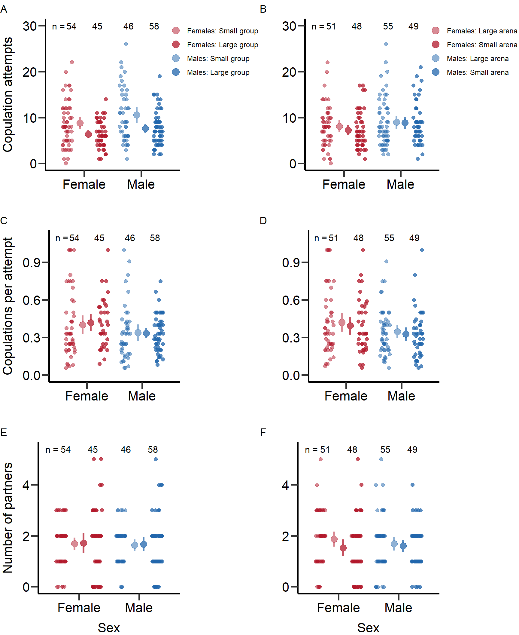
Figure S2: Mating behavior of males and females under low and high density manipulation via group (left) and arena size (right). Bars indicate means and 95% CI.
Figure_S2 = plot_grid(Figure_S2, ncol=1, rel_heights=c(0.1, 1)) # rel_heights values control title marginsFigure S3
#Behavior 2 (Figure S3)
Figure_S3<-grid.arrange(p6+labs(tag = "A")+xlab('')+theme(legend.position = c(1.25, 0.8),plot.margin = unit(c(0.2,3.5,0,0.1), "cm"),legend.text = element_text(size=9)),p6.2+labs(tag = "B")+xlab('')+theme(legend.position = c(1.25, 0.8),plot.margin = unit(c(0.2,3.5,0,0.1), "cm"),legend.text = element_text(size=9)),
                        p7+labs(tag = "C")+xlab('')+theme(legend.position = 'none',plot.margin = unit(c(0.2,3.5,0,0.1), "cm")),p7.2+labs(tag = "D")+xlab('')+theme(legend.position = 'none',plot.margin = unit(c(0.2,3.5,0,0.1), "cm")),
                        p8+labs(tag = "E")+xlab('Sex')+theme(legend.position = 'none',plot.margin = unit(c(0.2,3.5,0,0.1), "cm")),p8.2+labs(tag = "F")+xlab('Sex')+theme(legend.position = 'none',plot.margin = unit(c(0.2,3.5,0,0.1), "cm")),nrow = 3,ncol=2)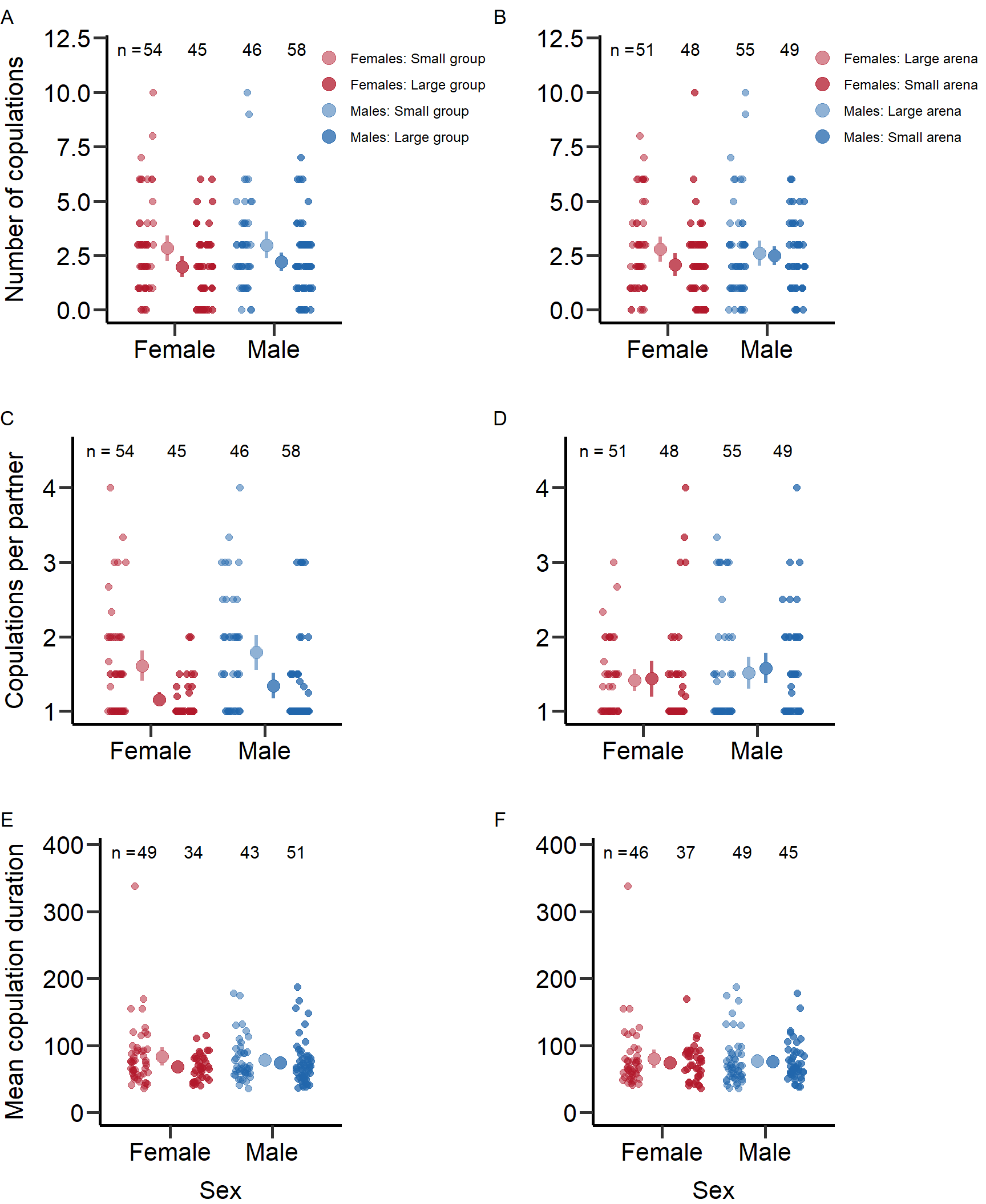
Figure S3: Mating behavior of males and females under low and high density manipulation via group (left) and arena size (right). Bars indicate means and 95% CI.
Figure_S3 = plot_grid(Figure_S3, ncol=1, rel_heights=c(0.1, 1)) # rel_heights values control title marginsFigure S4
# Reproductive success (Figure S4)
Figure_S4<-grid.arrange(grobs = list(p9+theme(legend.position = c(1.2, 0.8),plot.margin = unit(c(0.2,4,0,0.3), "cm")),p9.2+theme(legend.position = c(1.2, 0.8),plot.margin = unit(c(0.2,4,0,0.3), "cm"))), nrow = 1,ncol=2, widths=c(2.3, 2.3))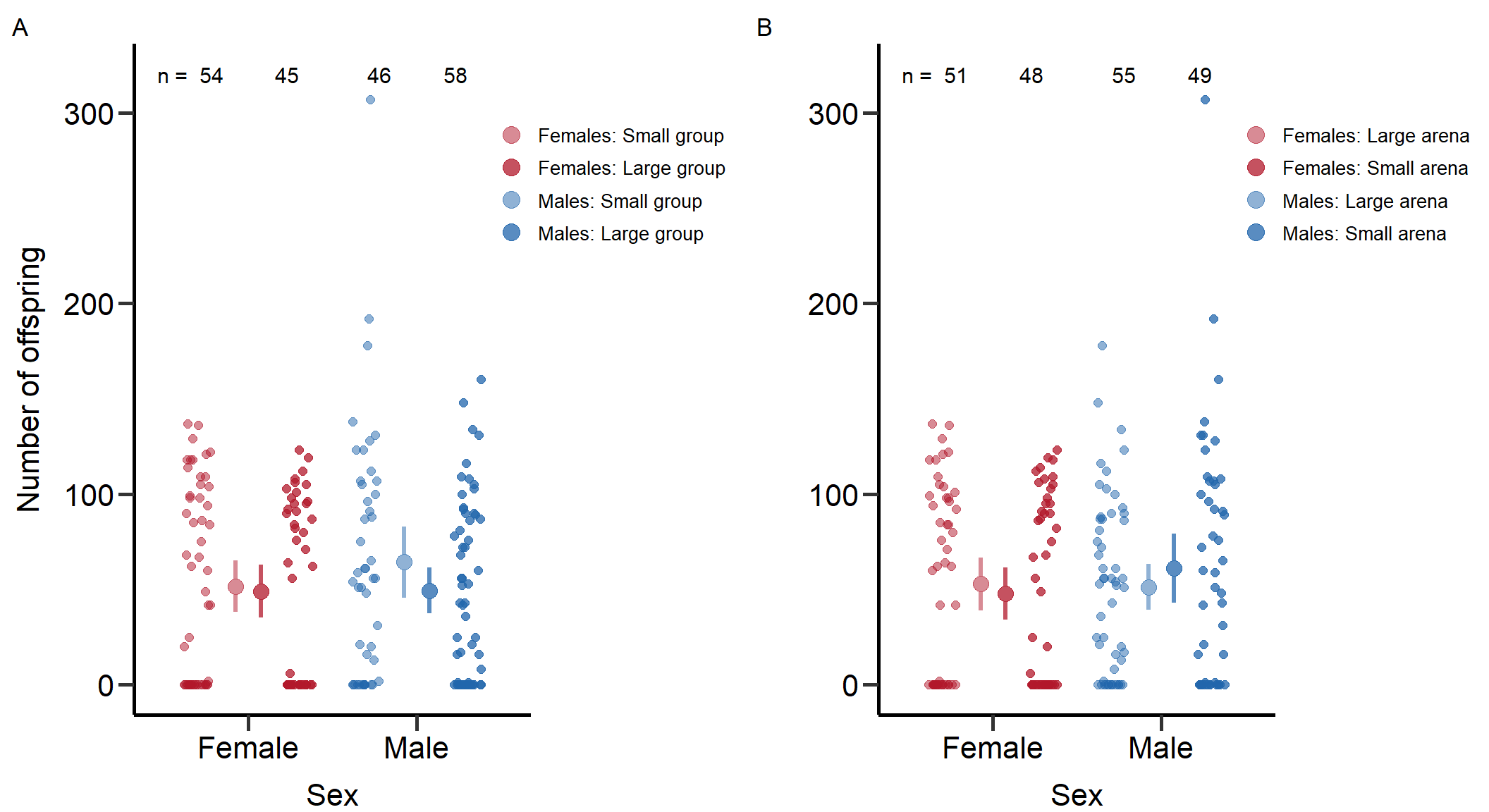
Figure S4: Reproductive success of males and females under density manipulation via group (left) and arena size (right). Bars indicate means and 95% CI.
Figure_S4 = plot_grid(Figure_S4, ncol=1, rel_heights=c(0.1, 1)) # rel_heights values control title marginsBootstrapping variances for mating behaviour and reproductive success
Next, we bootstrapped the coefficients of variation in mating behavior and reproductive success.
## Bootstrapping variances for mating behaviour and reproductive success ####
### Copulation attempts ####
# Male
# Large group size
D_data_Large_pop_M_MatingA_n <-as.vector(D_data_Large_pop$m_Total_Encounters)
c <- function(d, i){
  d2 <- d[i]
  return(sd(d2, na.rm=TRUE)/mean(d2, na.rm=TRUE))
}
Large_pop_M_MatingA_bootvar <- boot(D_data_Large_pop_M_MatingA_n, c, R=10000)

# Small group size
D_data_Small_pop_M_MatingA_n <-as.vector(D_data_Small_pop$m_Total_Encounters)

Small_pop_M_MatingA_bootvar <- boot(D_data_Small_pop_M_MatingA_n, c, R=10000)

# Large arena
D_data_Large_arena_M_MatingA_n <-as.vector(D_data_Large_arena$m_Total_Encounters)

Large_arena_M_MatingA_bootvar <- boot(D_data_Large_arena_M_MatingA_n, c, R=10000)

# Small arena
D_data_Small_arena_M_MatingA_n <-as.vector(D_data_Small_arena$m_Total_Encounters)

Small_arena_M_MatingA_bootvar <- boot(D_data_Small_arena_M_MatingA_n, c, R=10000)

# Female
# Large group size
D_data_Large_pop_F_MatingA_n <-as.vector(D_data_Large_pop$f_Total_Encounters)

Large_pop_F_MatingA_bootvar <- boot(D_data_Large_pop_F_MatingA_n, c, R=10000)

# Small group size
D_data_Small_pop_F_MatingA_n <-as.vector(D_data_Small_pop$f_Total_Encounters)

Small_pop_F_MatingA_bootvar <- boot(D_data_Small_pop_F_MatingA_n, c, R=10000)

# Large arena
D_data_Large_arena_F_MatingA_n <-as.vector(D_data_Large_arena$f_Total_Encounters)

Large_arena_F_MatingA_bootvar <- boot(D_data_Large_arena_F_MatingA_n, c, R=10000)

# Small arena
D_data_Small_arena_F_MatingA_n <-as.vector(D_data_Small_arena$f_Total_Encounters)

Small_arena_F_MatingA_bootvar <- boot(D_data_Small_arena_F_MatingA_n, c, R=10000)

### Copulations per encounter ####
# Male
# Large group size
D_data_Large_pop_M_PropSucCop_n <-as.vector(D_data_Large_pop$m_TotMatings/(D_data_Large_pop$m_TotMatings+D_data_Large_pop$m_Attempts_number))

Large_pop_M_PropSucCop_bootvar <- boot(D_data_Large_pop_M_PropSucCop_n, c, R=10000)

# Small group size
D_data_Small_pop_M_PropSucCop_n <-as.vector(D_data_Small_pop$m_TotMatings/(D_data_Small_pop$m_TotMatings+D_data_Small_pop$m_Attempts_number))

Small_pop_M_PropSucCop_bootvar <- boot(D_data_Small_pop_M_PropSucCop_n, c, R=10000)

# Small arena
D_data_Small_arena_M_PropSucCop_n <-as.vector(D_data_Small_arena$m_TotMatings/(D_data_Small_arena$m_TotMatings+D_data_Small_arena$m_Attempts_number))

Small_arena_M_PropSucCop_bootvar <- boot(D_data_Small_arena_M_PropSucCop_n, c, R=10000)

# Large arena
D_data_Large_arena_M_PropSucCop_n <-as.vector(D_data_Large_arena$m_TotMatings/(D_data_Large_arena$m_TotMatings+D_data_Large_arena$m_Attempts_number))

Large_arena_M_PropSucCop_bootvar <- boot(D_data_Large_arena_M_PropSucCop_n, c, R=10000)

# Female
# Large group size
D_data_Large_pop_F_PropSucCop_n <-as.vector(D_data_Large_pop$f_TotMatings/(D_data_Large_pop$f_TotMatings+D_data_Large_pop$f_Attempts_number))

Large_pop_F_PropSucCop_bootvar <- boot(D_data_Large_pop_F_PropSucCop_n, c, R=10000)

# Small group size
D_data_Small_pop_F_PropSucCop_n <-as.vector(D_data_Small_pop$f_TotMatings/(D_data_Small_pop$f_TotMatings+D_data_Small_pop$f_Attempts_number))

Small_pop_F_PropSucCop_bootvar <- boot(D_data_Small_pop_F_PropSucCop_n, c, R=10000)

# Small arena
D_data_Small_arena_F_PropSucCop_n <-as.vector(D_data_Small_arena$f_TotMatings/(D_data_Small_arena$f_TotMatings+D_data_Small_arena$f_Attempts_number))

Small_arena_F_PropSucCop_bootvar <- boot(D_data_Small_arena_F_PropSucCop_n, c, R=10000)

# Large arena
D_data_Large_arena_F_PropSucCop_n <-as.vector(D_data_Large_arena$f_TotMatings/(D_data_Large_arena$f_TotMatings+D_data_Large_arena$f_Attempts_number))

Large_arena_F_PropSucCop_bootvar <- boot(D_data_Large_arena_F_PropSucCop_n, c, R=10000)

### Number of partners ####
# Male
# Large group size
D_data_Large_pop_M_MS_n <-as.vector(D_data_Large_pop$m_cMS)

Large_pop_M_MS_bootvar <- boot(D_data_Large_pop_M_MS_n, c, R=10000)

# Small group size
D_data_Small_pop_M_MS_n <-as.vector(D_data_Small_pop$m_cMS)

Small_pop_M_MS_bootvar <- boot(D_data_Small_pop_M_MS_n, c, R=10000)

# Small arena
D_data_Small_arena_M_MS_n <-as.vector(D_data_Small_arena$m_cMS)

Small_arena_M_MS_bootvar <- boot(D_data_Small_arena_M_MS_n, c, R=10000)

# Large arena
D_data_Large_arena_M_MS_n <-as.vector(D_data_Large_arena$m_cMS)

Large_arena_M_MS_bootvar <- boot(D_data_Large_arena_M_MS_n, c, R=10000)

# Female
# Large group size
D_data_Large_pop_F_MS_n <-as.vector(D_data_Large_pop$f_cMS)

Large_pop_F_MS_bootvar <- boot(D_data_Large_pop_F_MS_n, c, R=10000)

# Small group size
D_data_Small_pop_F_MS_n <-as.vector(D_data_Small_pop$f_cMS)

Small_pop_F_MS_bootvar <- boot(D_data_Small_pop_F_MS_n, c, R=10000)

# Small arena
D_data_Small_arena_F_MS_n <-as.vector(D_data_Small_arena$f_cMS)

Small_arena_F_MS_bootvar <- boot(D_data_Small_arena_F_MS_n, c, R=10000)

# Large arena
D_data_Large_arena_F_MS_n <-as.vector(D_data_Large_arena$f_cMS)

Large_arena_F_MS_bootvar <- boot(D_data_Large_arena_F_MS_n, c, R=10000)

### Number of copulations ####
# Male
# Large group size
D_data_Large_pop_M_Matings_n <-as.vector(D_data_Large_pop$m_TotMatings)

Large_pop_M_Matings_bootvar <- boot(D_data_Large_pop_M_Matings_n, c, R=10000)

# Small group size
D_data_Small_pop_M_Matings_n <-as.vector(D_data_Small_pop$m_TotMatings)

Small_pop_M_Matings_bootvar <- boot(D_data_Small_pop_M_Matings_n, c, R=10000)

# Small arena
D_data_Small_arena_M_Matings_n <-as.vector(D_data_Small_arena$m_TotMatings)

Small_arena_M_Matings_bootvar <- boot(D_data_Small_arena_M_Matings_n, c, R=10000)

# Large arena
D_data_Large_arena_M_Matings_n <-as.vector(D_data_Large_arena$m_TotMatings)

Large_arena_M_Matings_bootvar <- boot(D_data_Large_arena_M_Matings_n, c, R=10000)

# Female
# Large group size
D_data_Large_pop_F_Matings_n <-as.vector(D_data_Large_pop$f_TotMatings)

Large_pop_F_Matings_bootvar <- boot(D_data_Large_pop_F_Matings_n, c, R=10000)

# Small group size
D_data_Small_pop_F_Matings_n <-as.vector(D_data_Small_pop$f_TotMatings)

Small_pop_F_Matings_bootvar <- boot(D_data_Small_pop_F_Matings_n, c, R=10000)

# Small arena
D_data_Small_arena_F_Matings_n <-as.vector(D_data_Small_arena$f_TotMatings)

Small_arena_F_Matings_bootvar <- boot(D_data_Small_arena_F_Matings_n, c, R=10000)

# Large arena
D_data_Large_arena_F_Matings_n <-as.vector(D_data_Large_arena$f_TotMatings)

Large_arena_F_Matings_bootvar <- boot(D_data_Large_arena_F_Matings_n, c, R=10000)

### Copulations per partner ####
# Male
# Large group size
D_data_Large_pop_M_MeanCop_n <-as.vector(D_data_Large_pop$m_meanCop)

Large_pop_M_MeanCop_bootvar <- boot(D_data_Large_pop_M_MeanCop_n, c, R=10000)

# Small group size
D_data_Small_pop_M_MeanCop_n <-as.vector(D_data_Small_pop$m_meanCop)

Small_pop_M_MeanCop_bootvar <- boot(D_data_Small_pop_M_MeanCop_n, c, R=10000)

# Small arena
D_data_Small_arena_M_MeanCop_n <-as.vector(D_data_Small_arena$m_meanCop)

Small_arena_M_MeanCop_bootvar <- boot(D_data_Small_arena_M_MeanCop_n, c, R=10000)

# Large arena
D_data_Large_arena_M_MeanCop_n <-as.vector(D_data_Large_arena$m_meanCop)

Large_arena_M_MeanCop_bootvar <- boot(D_data_Large_arena_M_MeanCop_n, c, R=10000)

# Female
# Large group size
D_data_Large_pop_F_MeanCop_n <-as.vector(D_data_Large_pop$f_meanCop)

Large_pop_F_MeanCop_bootvar <- boot(D_data_Large_pop_F_MeanCop_n, c, R=10000)

# Small group size
D_data_Small_pop_F_MeanCop_n <-as.vector(D_data_Small_pop$f_meanCop)

Small_pop_F_MeanCop_bootvar <- boot(D_data_Small_pop_F_MeanCop_n, c, R=10000)

# Small arena
D_data_Small_arena_F_MeanCop_n <-as.vector(D_data_Small_arena$f_meanCop)

Small_arena_F_MeanCop_bootvar <- boot(D_data_Small_arena_F_MeanCop_n, c, R=10000)

# Large arena
D_data_Large_arena_F_MeanCop_n <-as.vector(D_data_Large_arena$f_meanCop)

Large_arena_F_MeanCop_bootvar <- boot(D_data_Large_arena_F_MeanCop_n, c, R=10000)

### Mating duration ####
# Male
# Large group size
D_data_Large_pop_M_Duration_n <-as.vector(D_data_Large_pop$m_MatingDuration_av)

Large_pop_M_Duration_bootvar <- boot(D_data_Large_pop_M_Duration_n, c, R=10000)

# Small group size
D_data_Small_pop_M_Duration_n <-as.vector(D_data_Small_pop$m_MatingDuration_av)

Small_pop_M_Duration_bootvar <- boot(D_data_Small_pop_M_Duration_n, c, R=10000)

# Small arena
D_data_Small_arena_M_Duration_n <-as.vector(D_data_Small_arena$m_MatingDuration_av)

Small_arena_M_Duration_bootvar <- boot(D_data_Small_arena_M_Duration_n, c, R=10000)

# Large arena
D_data_Large_arena_M_Duration_n <-as.vector(D_data_Large_arena$m_MatingDuration_av)

Large_arena_M_Duration_bootvar <- boot(D_data_Large_arena_M_Duration_n, c, R=10000)

# Female
# Large group size
D_data_Large_pop_F_Duration_n <-as.vector(D_data_Large_pop$f_MatingDuration_av)

Large_pop_F_Duration_bootvar <- boot(D_data_Large_pop_F_Duration_n, c, R=10000)

# Small group size
D_data_Small_pop_F_Duration_n <-as.vector(D_data_Small_pop$f_MatingDuration_av)

Small_pop_F_Duration_bootvar <- boot(D_data_Small_pop_F_Duration_n, c, R=10000)

# Small arena
D_data_Small_arena_F_Duration_n <-as.vector(D_data_Small_arena$f_MatingDuration_av)

Small_arena_F_Duration_bootvar <- boot(D_data_Small_arena_F_Duration_n, c, R=10000)

# Large arena
D_data_Large_arena_F_Duration_n <-as.vector(D_data_Large_arena$f_MatingDuration_av)

Large_arena_F_Duration_bootvar <- boot(D_data_Large_arena_F_Duration_n, c, R=10000)

### Extract data and write results table ####
PhenVarBoot_Table_Male_Small_pop_MatingA <- as.data.frame(cbind("Male", "Small population size", "Copulation attempts", as.numeric(mean(Small_pop_M_MatingA_bootvar$t)), quantile(Small_pop_M_MatingA_bootvar$t,.025, names = FALSE), quantile(Small_pop_M_MatingA_bootvar$t,.975, names = FALSE)))
PhenVarBoot_Table_Male_Large_pop_MatingA <- as.data.frame(cbind("Male", "Large population size", "Copulation attempts", as.numeric(mean(Large_pop_M_MatingA_bootvar$t)), quantile(Large_pop_M_MatingA_bootvar$t,.025, names = FALSE), quantile(Large_pop_M_MatingA_bootvar$t,.975, names = FALSE)))
PhenVarBoot_Table_Female_Small_pop_MatingA <- as.data.frame(cbind("Female", "Small population size", "Copulation attempts", as.numeric(mean(Small_pop_F_MatingA_bootvar$t)), quantile(Small_pop_F_MatingA_bootvar$t,.025, names = FALSE), quantile(Small_pop_F_MatingA_bootvar$t,.975, names = FALSE)))
PhenVarBoot_Table_Female_Large_pop_MatingA <- as.data.frame(cbind("Female", "Large population size", "Copulation attempts", as.numeric(mean(Large_pop_F_MatingA_bootvar$t)), quantile(Large_pop_F_MatingA_bootvar$t,.025, names = FALSE), quantile(Large_pop_F_MatingA_bootvar$t,.975, names = FALSE)))
PhenVarBoot_Table_Male_Small_pop_PropSucCop <- as.data.frame(cbind("Male", "Small population size", "Copulations per encounter", as.numeric(mean(Small_pop_M_PropSucCop_bootvar$t)), quantile(Small_pop_M_PropSucCop_bootvar$t,.025, names = FALSE), quantile(Small_pop_M_PropSucCop_bootvar$t,.975, names = FALSE)))
PhenVarBoot_Table_Male_Large_pop_PropSucCop <- as.data.frame(cbind("Male", "Large population size", "Copulations per encounter", as.numeric(mean(Large_pop_M_PropSucCop_bootvar$t)), quantile(Large_pop_M_PropSucCop_bootvar$t,.025, names = FALSE), quantile(Large_pop_M_PropSucCop_bootvar$t,.975, names = FALSE)))
PhenVarBoot_Table_Female_Small_pop_PropSucCop <- as.data.frame(cbind("Female", "Small population size", "Copulations per encounter", as.numeric(mean(Small_pop_F_PropSucCop_bootvar$t)), quantile(Small_pop_F_PropSucCop_bootvar$t,.025, names = FALSE), quantile(Small_pop_F_PropSucCop_bootvar$t,.975, names = FALSE)))
PhenVarBoot_Table_Female_Large_pop_PropSucCop <- as.data.frame(cbind("Female", "Large population size", "Copulations per encounter", as.numeric(mean(Large_pop_F_PropSucCop_bootvar$t)), quantile(Large_pop_F_PropSucCop_bootvar$t,.025, names = FALSE), quantile(Large_pop_F_PropSucCop_bootvar$t,.975, names = FALSE)))
PhenVarBoot_Table_Male_Small_pop_Matings <- as.data.frame(cbind("Male", "Small population size", "Number copulations", as.numeric(mean(Small_pop_M_Matings_bootvar$t)), quantile(Small_pop_M_Matings_bootvar$t,.025, names = FALSE), quantile(Small_pop_M_Matings_bootvar$t,.975, names = FALSE)))
PhenVarBoot_Table_Male_Large_pop_Matings <- as.data.frame(cbind("Male", "Large population size", "Number copulations", as.numeric(mean(Large_pop_M_Matings_bootvar$t)), quantile(Large_pop_M_Matings_bootvar$t,.025, names = FALSE), quantile(Large_pop_M_Matings_bootvar$t,.975, names = FALSE)))
PhenVarBoot_Table_Female_Small_pop_Matings <- as.data.frame(cbind("Female", "Small population size", "Number copulations", as.numeric(mean(Small_pop_F_Matings_bootvar$t)), quantile(Small_pop_F_Matings_bootvar$t,.025, names = FALSE), quantile(Small_pop_F_Matings_bootvar$t,.975, names = FALSE)))
PhenVarBoot_Table_Female_Large_pop_Matings <- as.data.frame(cbind("Female", "Large population size", "Number copulations", as.numeric(mean(Large_pop_F_Matings_bootvar$t)), quantile(Large_pop_F_Matings_bootvar$t,.025, names = FALSE), quantile(Large_pop_F_Matings_bootvar$t,.975, names = FALSE)))
PhenVarBoot_Table_Male_Small_pop_MS <- as.data.frame(cbind("Male", "Small population size", "Number of partners", as.numeric(mean(Small_pop_M_MS_bootvar$t)), quantile(Small_pop_M_MS_bootvar$t,.025, names = FALSE), quantile(Small_pop_M_MS_bootvar$t,.975, names = FALSE)))
PhenVarBoot_Table_Male_Large_pop_MS <- as.data.frame(cbind("Male", "Large population size", "Number of partners", as.numeric(mean(Large_pop_M_MS_bootvar$t)), quantile(Large_pop_M_MS_bootvar$t,.025, names = FALSE), quantile(Large_pop_M_MS_bootvar$t,.975, names = FALSE)))
PhenVarBoot_Table_Female_Small_pop_MS <- as.data.frame(cbind("Female", "Small population size", "Number of partners", as.numeric(mean(Small_pop_F_MS_bootvar$t)), quantile(Small_pop_F_MS_bootvar$t,.025, names = FALSE), quantile(Small_pop_F_MS_bootvar$t,.975, names = FALSE)))
PhenVarBoot_Table_Female_Large_pop_MS <- as.data.frame(cbind("Female", "Large population size", "Number of partners", as.numeric(mean(Large_pop_F_MS_bootvar$t)), quantile(Large_pop_F_MS_bootvar$t,.025, names = FALSE), quantile(Large_pop_F_MS_bootvar$t,.975, names = FALSE)))
PhenVarBoot_Table_Male_Small_pop_MeanCop <- as.data.frame(cbind("Male", "Small population size", "Copulations per partner", as.numeric(mean(Small_pop_M_MeanCop_bootvar$t)), quantile(Small_pop_M_MeanCop_bootvar$t,.025, names = FALSE), quantile(Small_pop_M_MeanCop_bootvar$t,.975, names = FALSE)))
PhenVarBoot_Table_Male_Large_pop_MeanCop <- as.data.frame(cbind("Male", "Large population size", "Copulations per partner", as.numeric(mean(Large_pop_M_MeanCop_bootvar$t)), quantile(Large_pop_M_MeanCop_bootvar$t,.025, names = FALSE), quantile(Large_pop_M_MeanCop_bootvar$t,.975, names = FALSE)))
PhenVarBoot_Table_Female_Small_pop_MeanCop <- as.data.frame(cbind("Female", "Small population size", "Copulations per partner", as.numeric(mean(Small_pop_F_MeanCop_bootvar$t)), quantile(Small_pop_F_MeanCop_bootvar$t,.025, names = FALSE), quantile(Small_pop_F_MeanCop_bootvar$t,.975, names = FALSE)))
PhenVarBoot_Table_Female_Large_pop_MeanCop <- as.data.frame(cbind("Female", "Large population size", "Copulations per partner", as.numeric(mean(Large_pop_F_MeanCop_bootvar$t)), quantile(Large_pop_F_MeanCop_bootvar$t,.025, names = FALSE), quantile(Large_pop_F_MeanCop_bootvar$t,.975, names = FALSE)))
PhenVarBoot_Table_Male_Small_pop_Duration <- as.data.frame(cbind("Male", "Small population size", "Copulation duration", as.numeric(mean(Small_pop_M_Duration_bootvar$t)), quantile(Small_pop_M_Duration_bootvar$t,.025, names = FALSE), quantile(Small_pop_M_Duration_bootvar$t,.975, names = FALSE)))
PhenVarBoot_Table_Male_Large_pop_Duration <- as.data.frame(cbind("Male", "Large population size", "Copulation duration", as.numeric(mean(Large_pop_M_Duration_bootvar$t)), quantile(Large_pop_M_Duration_bootvar$t,.025, names = FALSE), quantile(Large_pop_M_Duration_bootvar$t,.975, names = FALSE)))
PhenVarBoot_Table_Female_Small_pop_Duration <- as.data.frame(cbind("Female", "Small population size", "Copulation duration", as.numeric(mean(Small_pop_F_Duration_bootvar$t)), quantile(Small_pop_F_Duration_bootvar$t,.025, names = FALSE), quantile(Small_pop_F_Duration_bootvar$t,.975, names = FALSE)))
PhenVarBoot_Table_Female_Large_pop_Duration <- as.data.frame(cbind("Female", "Large population size", "Copulation duration", as.numeric(mean(Large_pop_F_Duration_bootvar$t)), quantile(Large_pop_F_Duration_bootvar$t,.025, names = FALSE), quantile(Large_pop_F_Duration_bootvar$t,.975, names = FALSE)))

PhenVarBoot_Table_Male_Small_arena_MatingA <- as.data.frame(cbind("Male", "Small arena size", "Copulation attempts", as.numeric(mean(Small_arena_M_MatingA_bootvar$t)), quantile(Small_arena_M_MatingA_bootvar$t,.025, names = FALSE), quantile(Small_arena_M_MatingA_bootvar$t,.975, names = FALSE)))
PhenVarBoot_Table_Male_Large_arena_MatingA <- as.data.frame(cbind("Male", "Large arena size", "Copulation attempts", as.numeric(mean(Large_arena_M_MatingA_bootvar$t)), quantile(Large_arena_M_MatingA_bootvar$t,.025, names = FALSE), quantile(Large_arena_M_MatingA_bootvar$t,.975, names = FALSE)))
PhenVarBoot_Table_Female_Small_arena_MatingA <- as.data.frame(cbind("Female", "Small arena size", "Copulation attempts", as.numeric(mean(Small_arena_F_MatingA_bootvar$t)), quantile(Small_arena_F_MatingA_bootvar$t,.025, names = FALSE), quantile(Small_arena_F_MatingA_bootvar$t,.975, names = FALSE)))
PhenVarBoot_Table_Female_Large_arena_MatingA <- as.data.frame(cbind("Female", "Large arena size", "Copulation attempts", as.numeric(mean(Large_arena_F_MatingA_bootvar$t)), quantile(Large_arena_F_MatingA_bootvar$t,.025, names = FALSE), quantile(Large_arena_F_MatingA_bootvar$t,.975, names = FALSE)))
PhenVarBoot_Table_Male_Small_arena_PropSucCop <- as.data.frame(cbind("Male", "Small arena size", "Copulations per encounter", as.numeric(mean(Small_arena_M_PropSucCop_bootvar$t)), quantile(Small_arena_M_PropSucCop_bootvar$t,.025, names = FALSE), quantile(Small_arena_M_PropSucCop_bootvar$t,.975, names = FALSE)))
PhenVarBoot_Table_Male_Large_arena_PropSucCop <- as.data.frame(cbind("Male", "Large arena size", "Copulations per encounter", as.numeric(mean(Large_arena_M_PropSucCop_bootvar$t)), quantile(Large_arena_M_PropSucCop_bootvar$t,.025, names = FALSE), quantile(Large_arena_M_PropSucCop_bootvar$t,.975, names = FALSE)))
PhenVarBoot_Table_Female_Small_arena_PropSucCop <- as.data.frame(cbind("Female", "Small arena size", "Copulations per encounter", as.numeric(mean(Small_arena_F_PropSucCop_bootvar$t)), quantile(Small_arena_F_PropSucCop_bootvar$t,.025, names = FALSE), quantile(Small_arena_F_PropSucCop_bootvar$t,.975, names = FALSE)))
PhenVarBoot_Table_Female_Large_arena_PropSucCop <- as.data.frame(cbind("Female", "Large arena size", "Copulations per encounter", as.numeric(mean(Large_arena_F_PropSucCop_bootvar$t)), quantile(Large_arena_F_PropSucCop_bootvar$t,.025, names = FALSE), quantile(Large_arena_F_PropSucCop_bootvar$t,.975, names = FALSE)))
PhenVarBoot_Table_Male_Small_arena_Matings <- as.data.frame(cbind("Male", "Small arena size", "Number copulations", as.numeric(mean(Small_arena_M_Matings_bootvar$t)), quantile(Small_arena_M_Matings_bootvar$t,.025, names = FALSE), quantile(Small_arena_M_Matings_bootvar$t,.975, names = FALSE)))
PhenVarBoot_Table_Male_Large_arena_Matings <- as.data.frame(cbind("Male", "Large arena size", "Number copulations", as.numeric(mean(Large_arena_M_Matings_bootvar$t)), quantile(Large_arena_M_Matings_bootvar$t,.025, names = FALSE), quantile(Large_arena_M_Matings_bootvar$t,.975, names = FALSE)))
PhenVarBoot_Table_Female_Small_arena_Matings <- as.data.frame(cbind("Female", "Small arena size", "Number copulations", as.numeric(mean(Small_arena_F_Matings_bootvar$t)), quantile(Small_arena_F_Matings_bootvar$t,.025, names = FALSE), quantile(Small_arena_F_Matings_bootvar$t,.975, names = FALSE)))
PhenVarBoot_Table_Female_Large_arena_Matings <- as.data.frame(cbind("Female", "Large arena size", "Number copulations", as.numeric(mean(Large_arena_F_Matings_bootvar$t)), quantile(Large_arena_F_Matings_bootvar$t,.025, names = FALSE), quantile(Large_arena_F_Matings_bootvar$t,.975, names = FALSE)))
PhenVarBoot_Table_Male_Small_arena_MeanCop <- as.data.frame(cbind("Male", "Small arena size", "Copulations per partner", as.numeric(mean(Small_arena_M_MeanCop_bootvar$t)), quantile(Small_arena_M_MeanCop_bootvar$t,.025, names = FALSE), quantile(Small_arena_M_MeanCop_bootvar$t,.975, names = FALSE)))
PhenVarBoot_Table_Male_Large_arena_MeanCop <- as.data.frame(cbind("Male", "Large arena size", "Copulations per partner", as.numeric(mean(Large_arena_M_MeanCop_bootvar$t)), quantile(Large_arena_M_MeanCop_bootvar$t,.025, names = FALSE), quantile(Large_arena_M_MeanCop_bootvar$t,.975, names = FALSE)))
PhenVarBoot_Table_Female_Small_arena_MeanCop <- as.data.frame(cbind("Female", "Small arena size", "Copulations per partner", as.numeric(mean(Small_arena_F_MeanCop_bootvar$t)), quantile(Small_arena_F_MeanCop_bootvar$t,.025, names = FALSE), quantile(Small_arena_F_MeanCop_bootvar$t,.975, names = FALSE)))
PhenVarBoot_Table_Female_Large_arena_MeanCop <- as.data.frame(cbind("Female", "Large arena size", "Copulations per partner", as.numeric(mean(Large_arena_F_MeanCop_bootvar$t)), quantile(Large_arena_F_MeanCop_bootvar$t,.025, names = FALSE), quantile(Large_arena_F_MeanCop_bootvar$t,.975, names = FALSE)))
PhenVarBoot_Table_Male_Small_arena_Duration <- as.data.frame(cbind("Male", "Small arena size", "Copulation duration", as.numeric(mean(Small_arena_M_Duration_bootvar$t)), quantile(Small_arena_M_Duration_bootvar$t,.025, names = FALSE), quantile(Small_arena_M_Duration_bootvar$t,.975, names = FALSE)))
PhenVarBoot_Table_Male_Large_arena_Duration <- as.data.frame(cbind("Male", "Large arena size", "Copulation duration", as.numeric(mean(Large_arena_M_Duration_bootvar$t)), quantile(Large_arena_M_Duration_bootvar$t,.025, names = FALSE), quantile(Large_arena_M_Duration_bootvar$t,.975, names = FALSE)))
PhenVarBoot_Table_Female_Small_arena_Duration <- as.data.frame(cbind("Female", "Small arena size", "Copulation duration", as.numeric(mean(Small_arena_F_Duration_bootvar$t)), quantile(Small_arena_F_Duration_bootvar$t,.025, names = FALSE), quantile(Small_arena_F_Duration_bootvar$t,.975, names = FALSE)))
PhenVarBoot_Table_Female_Large_arena_Duration <- as.data.frame(cbind("Female", "Large arena size", "Copulation duration", as.numeric(mean(Large_arena_F_Duration_bootvar$t)), quantile(Large_arena_F_Duration_bootvar$t,.025, names = FALSE), quantile(Large_arena_F_Duration_bootvar$t,.975, names = FALSE)))
PhenVarBoot_Table_Male_Small_arena_MS <- as.data.frame(cbind("Male", "Small arena size", "Number of partners", as.numeric(mean(Small_arena_M_MS_bootvar$t)), quantile(Small_arena_M_MS_bootvar$t,.025, names = FALSE), quantile(Small_arena_M_MS_bootvar$t,.975, names = FALSE)))
PhenVarBoot_Table_Male_Large_arena_MS <- as.data.frame(cbind("Male", "Large arena size", "Number of partners", as.numeric(mean(Large_arena_M_MS_bootvar$t)), quantile(Large_arena_M_MS_bootvar$t,.025, names = FALSE), quantile(Large_arena_M_MS_bootvar$t,.975, names = FALSE)))
PhenVarBoot_Table_Female_Small_arena_MS <- as.data.frame(cbind("Female", "Small arena size", "Number of partners", as.numeric(mean(Small_arena_F_MS_bootvar$t)), quantile(Small_arena_F_MS_bootvar$t,.025, names = FALSE), quantile(Small_arena_F_MS_bootvar$t,.975, names = FALSE)))
PhenVarBoot_Table_Female_Large_arena_MS <- as.data.frame(cbind("Female", "Large arena size", "Number of partners", as.numeric(mean(Large_arena_F_MS_bootvar$t)), quantile(Large_arena_F_MS_bootvar$t,.025, names = FALSE), quantile(Large_arena_F_MS_bootvar$t,.975, names = FALSE)))

Table_VarBeh <- as.data.frame(as.matrix(rbind(PhenVarBoot_Table_Male_Small_pop_MatingA,PhenVarBoot_Table_Male_Large_pop_MatingA,
                                              PhenVarBoot_Table_Female_Small_pop_MatingA,PhenVarBoot_Table_Female_Large_pop_MatingA,
                                              PhenVarBoot_Table_Male_Small_pop_PropSucCop,PhenVarBoot_Table_Male_Large_pop_PropSucCop,
                                              PhenVarBoot_Table_Female_Small_pop_PropSucCop,PhenVarBoot_Table_Female_Large_pop_PropSucCop,
                                              PhenVarBoot_Table_Male_Small_pop_Matings,PhenVarBoot_Table_Male_Large_pop_Matings,
                                              PhenVarBoot_Table_Female_Small_pop_Matings,PhenVarBoot_Table_Female_Large_pop_Matings,
                                              PhenVarBoot_Table_Male_Small_pop_MeanCop,PhenVarBoot_Table_Male_Large_pop_MeanCop,
                                              PhenVarBoot_Table_Female_Small_pop_MeanCop,PhenVarBoot_Table_Female_Large_pop_MeanCop,
                                              PhenVarBoot_Table_Male_Small_pop_Duration,PhenVarBoot_Table_Male_Large_pop_Duration,
                                              PhenVarBoot_Table_Female_Small_pop_Duration,PhenVarBoot_Table_Female_Large_pop_Duration,
                                              PhenVarBoot_Table_Male_Small_arena_MatingA,PhenVarBoot_Table_Male_Large_arena_MatingA,
                                              PhenVarBoot_Table_Female_Small_arena_MatingA,PhenVarBoot_Table_Female_Large_arena_MatingA,
                                              PhenVarBoot_Table_Male_Small_arena_PropSucCop,PhenVarBoot_Table_Male_Large_arena_PropSucCop,
                                              PhenVarBoot_Table_Female_Small_arena_PropSucCop,PhenVarBoot_Table_Female_Large_arena_PropSucCop,
                                              PhenVarBoot_Table_Male_Small_arena_Matings,PhenVarBoot_Table_Male_Large_arena_Matings,
                                              PhenVarBoot_Table_Female_Small_arena_Matings,PhenVarBoot_Table_Female_Large_arena_Matings,
                                              PhenVarBoot_Table_Male_Small_arena_MeanCop,PhenVarBoot_Table_Male_Large_arena_MeanCop,
                                              PhenVarBoot_Table_Female_Small_arena_MeanCop,PhenVarBoot_Table_Female_Large_arena_MeanCop,
                                              PhenVarBoot_Table_Male_Small_arena_Duration,PhenVarBoot_Table_Male_Large_arena_Duration,
                                              PhenVarBoot_Table_Female_Small_arena_Duration,PhenVarBoot_Table_Female_Large_arena_Duration,
                                              PhenVarBoot_Table_Male_Small_pop_MS,PhenVarBoot_Table_Male_Large_pop_MS,
                                              PhenVarBoot_Table_Female_Small_pop_MS,PhenVarBoot_Table_Female_Large_pop_MS,
                                              PhenVarBoot_Table_Male_Small_arena_MS,PhenVarBoot_Table_Male_Large_arena_MS,
                                              PhenVarBoot_Table_Female_Small_arena_MS,PhenVarBoot_Table_Female_Large_arena_MS)),digits=3)

is.table(Table_VarBeh)
colnames(Table_VarBeh)[1] <- "Sex"
colnames(Table_VarBeh)[2] <- "Treatment"
colnames(Table_VarBeh)[3] <- "Variable"
colnames(Table_VarBeh)[4] <- "Variance"
colnames(Table_VarBeh)[5] <- "l95_CI"
colnames(Table_VarBeh)[6] <- "u95_CI"
Table_VarBeh[,4]=round(as.numeric(Table_VarBeh[,4]),digits=2)
Table_VarBeh[,5]=round(as.numeric(Table_VarBeh[,5]),digits=2)
Table_VarBeh[,6]=round(as.numeric(Table_VarBeh[,6]),digits=2)

rm(c) # Remove bootstrapping function
Table S5: Coefficients of variation (CV) in mating behavior for treatments (group and arena size) estimated for males and females with mean and 95%CI estimated via bootstrapping.
kable(Table_VarBeh)| Sex | Treatment | Variable | Variance | l95_CI | u95_CI |
|---|---|---|---|---|---|
| Male | Small population size | Copulation attempts | 0.59 | 0.47 | 0.71 |
| Male | Large population size | Copulation attempts | 0.48 | 0.40 | 0.57 |
| Female | Small population size | Copulation attempts | 0.56 | 0.46 | 0.67 |
| Female | Large population size | Copulation attempts | 0.46 | 0.37 | 0.56 |
| Male | Small population size | Copulations per encounter | 0.71 | 0.56 | 0.87 |
| Male | Large population size | Copulations per encounter | 0.60 | 0.47 | 0.74 |
| Female | Small population size | Copulations per encounter | 0.74 | 0.61 | 0.87 |
| Female | Large population size | Copulations per encounter | 0.79 | 0.60 | 1.01 |
| Male | Small population size | Number copulations | 0.70 | 0.54 | 0.86 |
| Male | Large population size | Number copulations | 0.72 | 0.59 | 0.87 |
| Female | Small population size | Number copulations | 0.76 | 0.62 | 0.92 |
| Female | Large population size | Number copulations | 0.83 | 0.65 | 1.04 |
| Male | Small population size | Copulations per partner | 0.43 | 0.35 | 0.51 |
| Male | Large population size | Copulations per partner | 0.46 | 0.34 | 0.53 |
| Female | Small population size | Copulations per partner | 0.44 | 0.35 | 0.52 |
| Female | Large population size | Copulations per partner | 0.29 | 0.17 | 0.42 |
| Male | Small population size | Copulation duration | 0.39 | 0.29 | 0.48 |
| Male | Large population size | Copulation duration | 0.44 | 0.33 | 0.53 |
| Female | Small population size | Copulation duration | 0.54 | 0.33 | 0.77 |
| Female | Large population size | Copulation duration | 0.28 | 0.22 | 0.34 |
| Male | Small arena size | Copulation attempts | 0.58 | 0.44 | 0.73 |
| Male | Large arena size | Copulation attempts | 0.59 | 0.49 | 0.69 |
| Female | Small arena size | Copulation attempts | 0.54 | 0.45 | 0.64 |
| Female | Large arena size | Copulation attempts | 0.56 | 0.44 | 0.69 |
| Male | Small arena size | Copulations per encounter | 0.66 | 0.50 | 0.82 |
| Male | Large arena size | Copulations per encounter | 0.66 | 0.53 | 0.80 |
| Female | Small arena size | Copulations per encounter | 0.83 | 0.66 | 1.04 |
| Female | Large arena size | Copulations per encounter | 0.69 | 0.57 | 0.83 |
| Male | Small arena size | Number copulations | 0.61 | 0.49 | 0.74 |
| Male | Large arena size | Number copulations | 0.82 | 0.66 | 0.99 |
| Female | Small arena size | Number copulations | 0.87 | 0.63 | 1.14 |
| Female | Large arena size | Number copulations | 0.74 | 0.61 | 0.88 |
| Male | Small arena size | Copulations per partner | 0.44 | 0.34 | 0.54 |
| Male | Large arena size | Copulations per partner | 0.50 | 0.43 | 0.55 |
| Female | Small arena size | Copulations per partner | 0.53 | 0.36 | 0.67 |
| Female | Large arena size | Copulations per partner | 0.35 | 0.28 | 0.42 |
| Male | Small arena size | Copulation duration | 0.38 | 0.27 | 0.47 |
| Male | Large arena size | Copulation duration | 0.45 | 0.35 | 0.54 |
| Female | Small arena size | Copulation duration | 0.35 | 0.25 | 0.45 |
| Female | Large arena size | Copulation duration | 0.55 | 0.31 | 0.81 |
| Male | Small population size | Number of partners | 0.47 | 0.36 | 0.59 |
| Male | Large population size | Number of partners | 0.62 | 0.49 | 0.77 |
| Female | Small population size | Number of partners | 0.52 | 0.41 | 0.65 |
| Female | Large population size | Number of partners | 0.78 | 0.60 | 0.98 |
| Male | Small arena size | Number of partners | 0.51 | 0.38 | 0.64 |
| Male | Large arena size | Number of partners | 0.60 | 0.47 | 0.75 |
| Female | Small arena size | Number of partners | 0.74 | 0.57 | 0.93 |
| Female | Large arena size | Number of partners | 0.57 | 0.45 | 0.71 |
Figure of variance in mating behaviour (Figure S5)
We plotted the coefficients of variation in mating behavior and reproductive success.
## Figure of variance in mating behaviour (Figure S5) ####
### Plot: Variance in copulation attempts ####
# Reorder data
plot_MatingA_data_1=Table_VarBeh[c(1,3,22,24),c(1,2,4,5,6)]
names(plot_MatingA_data_1)[3] <- "Variance_low"
names(plot_MatingA_data_1)[4] <- "lCI_low"
names(plot_MatingA_data_1)[5] <- "uCI_low"
plot_MatingA_data_2=Table_VarBeh[c(2,4,21,23),c(4,5,6)]
names(plot_MatingA_data_2)[1] <- "Variance_high"
names(plot_MatingA_data_2)[2] <- "lCI_high"
names(plot_MatingA_data_2)[3] <- "uCI_high"
plot_MatingA_data=cbind(plot_MatingA_data_1,plot_MatingA_data_2)
plot_MatingA_data[c(1,2),2]='Group size'
plot_MatingA_data[c(3,4),2]='Arena size'

p10=ggplot(plot_MatingA_data, aes(x=Variance_low, y=Variance_high, color=Sex, shape=Treatment)) +geom_abline(intercept = 0, slope = 1,size=1,linetype=2) +
  annotate(geom = "polygon", x = c(Inf, -Inf, -Inf), y = c(Inf, -Inf, Inf), fill = "grey", alpha = 0.2 )+
  geom_point(size = 5,alpha=1)+
  geom_errorbar(alpha=0.5,size=1.1,width=0, orientation='y',aes(xmin=lCI_low, xmax=uCI_low),show.legend=FALSE) +geom_errorbar(alpha=0.5,size=1.1,width=0, orientation='x', aes(ymin=lCI_high, ymax=uCI_high),show.legend=FALSE)+
  ylab((('High density \nCV copulation attempts')))+labs(tag = "A")+xlab((('Low density \nCV copulation attempts')))+
  scale_shape_manual(values=c(15, 19))+
  scale_color_manual(values=colpal2)+
  guides(shape = guide_legend(override.aes = list(size = 3.5)))+
  xlim(0.15,1.15)+ylim(0.15,1.15)+
  guides(shape = guide_legend(override.aes = list(size = 5)))+
  theme(panel.border = element_blank(),
        plot.title = element_text(hjust = 0.5),
        panel.background = element_blank(),
        panel.grid.major = element_blank(),
        panel.grid.minor = element_blank(),
        plot.tag.position=c(0.01,0.98),
        legend.position = c(0.8, 0.4),
        legend.spacing.y = unit(0.1, 'cm'),
        legend.key=element_blank(),
        legend.title = element_blank(),
        legend.margin = margin(0,0,0,0, unit="cm"),
        legend.text = element_text(colour="black", size=11),
        axis.line.x = element_line(colour = "black", size = 1),
        axis.line.y = element_line(colour = "black", size = 1),
        axis.text.x = element_text(face="plain", color="black", size=16, angle=0),
        axis.text.y = element_text(face="plain", color="black", size=16, angle=0),
        axis.title.x = element_text(size=16,face="plain", margin = margin(r=0,10,0,0)),
        axis.title.y = element_text(size=16,face="plain", margin = margin(r=10,0,0,0)),
        axis.ticks = element_line(size = 1),
        axis.ticks.length = unit(.3, "cm"),
        plot.margin = unit(c(0.5,0.2,0.1,0.2), "cm"))

### Plot: Varince in copulations per encounter ####
# Reorder data
plot_PropSuc_data_1=Table_VarBeh[c(5,7,26,28),c(1,2,4,5,6)]
names(plot_PropSuc_data_1)[3] <- "Variance_low"
names(plot_PropSuc_data_1)[4] <- "lCI_low"
names(plot_PropSuc_data_1)[5] <- "uCI_low"
plot_PropSuc_data_2=Table_VarBeh[c(6,8,25,27),c(4,5,6)]
names(plot_PropSuc_data_2)[1] <- "Variance_high"
names(plot_PropSuc_data_2)[2] <- "lCI_high"
names(plot_PropSuc_data_2)[3] <- "uCI_high"
plot_PropSuc_data=cbind(plot_PropSuc_data_1,plot_PropSuc_data_2)
plot_PropSuc_data[c(1,2),2]='Group size'
plot_PropSuc_data[c(3,4),2]='Arena'

p11=ggplot(plot_PropSuc_data, aes(x=Variance_low, y=Variance_high, color=Sex, shape=Treatment)) +geom_abline(intercept = 0, slope = 1,size=1,linetype=2) +
  annotate(geom = "polygon", x = c(Inf, -Inf, -Inf), y = c(Inf, -Inf, Inf), fill = "grey", alpha = 0.2 )+
  geom_point(size = 5,alpha=1)+
  geom_errorbar(alpha=0.5,size=1.1,width=0, orientation='y',aes(xmin=lCI_low, xmax=uCI_low),show.legend=FALSE) +geom_errorbar(alpha=0.5,size=1.1,width=0, orientation='x', aes(ymin=lCI_high, ymax=uCI_high),show.legend=FALSE)+
  ylab((('High density \nCV copulations per encounter')))+labs(tag = "B")+xlab((('Low density \nCV copulations per encounter')))+
  scale_shape_manual(values=c(15, 19))+
  scale_color_manual(values=colpal2)+
  guides(shape = guide_legend(override.aes = list(size = 3.5)))+
  xlim(0.15,1.15)+ylim(0.15,1.15)+
  guides(shape = guide_legend(override.aes = list(size = 5)))+
   theme(panel.border = element_blank(),
        plot.title = element_text(hjust = 0.5),
        panel.background = element_blank(),
        panel.grid.major = element_blank(),
        panel.grid.minor = element_blank(),
        plot.tag.position=c(0.01,0.98),
        legend.position = 'none',
        legend.spacing.y = unit(0.1, 'cm'),
        legend.key=element_blank(),
        legend.title = element_blank(),
        legend.margin = margin(0,0,0,0, unit="cm"),
        legend.text = element_text(colour="black", size=11),
        axis.line.x = element_line(colour = "black", size = 1),
        axis.line.y = element_line(colour = "black", size = 1),
        axis.text.x = element_text(face="plain", color="black", size=16, angle=0),
        axis.text.y = element_text(face="plain", color="black", size=16, angle=0),
        axis.title.x = element_text(size=16,face="plain", margin = margin(r=0,10,0,0)),
        axis.title.y = element_text(size=16,face="plain", margin = margin(r=10,0,0,0)),
        axis.ticks = element_line(size = 1),
        axis.ticks.length = unit(.3, "cm"),
        plot.margin = unit(c(0.5,0.2,0.1,0.2), "cm"))

### Plot: Variance in mating success ####
# Reorder data
plot_MS_data_1=Table_VarBeh[c(41,43,46,48),c(1,2,4,5,6)]
names(plot_MS_data_1)[3] <- "Variance_low"
names(plot_MS_data_1)[4] <- "lCI_low"
names(plot_MS_data_1)[5] <- "uCI_low"
plot_MS_data_2=Table_VarBeh[c(42,44,45,47),c(4,5,6)]
names(plot_MS_data_2)[1] <- "Variance_high"
names(plot_MS_data_2)[2] <- "lCI_high"
names(plot_MS_data_2)[3] <- "uCI_high"
plot_MS_data=cbind(plot_MS_data_1,plot_MS_data_2)
plot_MS_data[c(1,2),2]='Group size'
plot_MS_data[c(3,4),2]='Arena'

p12=ggplot(plot_MS_data, aes(x=Variance_low, y=Variance_high, color=Sex, shape=Treatment)) +geom_abline(intercept = 0, slope = 1,size=1,linetype=2) +
  annotate(geom = "polygon", x = c(Inf, -Inf, -Inf), y = c(Inf, -Inf, Inf), fill = "grey", alpha = 0.2 )+
  geom_point(size = 5,alpha=1)+
  geom_errorbar(alpha=0.5,size=1.1,width=0, orientation='y',aes(xmin=lCI_low, xmax=uCI_low)) +geom_errorbar(alpha=0.5,size=1.1,width=0, orientation='x', aes(ymin=lCI_high, ymax=uCI_high))+
  ylab((('High density \nCV number of partners')))+labs(tag = "C")+xlab((('Low density \nCV number of partners')))+
  scale_shape_manual(values=c(15, 19))+
  scale_color_manual(values=colpal2)+
  guides(shape = guide_legend(override.aes = list(size = 3.5)))+
  xlim(0.15,1.15)+ylim(0.15,1.15)+
  guides(shape = guide_legend(override.aes = list(size = 5)))+
   theme(panel.border = element_blank(),
        plot.title = element_text(hjust = 0.5),
        panel.background = element_blank(),
        panel.grid.major = element_blank(),
        panel.grid.minor = element_blank(),
        plot.tag.position=c(0.01,0.98),
        legend.position = 'none',
        legend.spacing.y = unit(0.1, 'cm'),
        legend.key=element_blank(),
        legend.title = element_blank(),
        legend.margin = margin(0,0,0,0, unit="cm"),
        legend.text = element_text(colour="black", size=11),
        axis.line.x = element_line(colour = "black", size = 1),
        axis.line.y = element_line(colour = "black", size = 1),
        axis.text.x = element_text(face="plain", color="black", size=16, angle=0),
        axis.text.y = element_text(face="plain", color="black", size=16, angle=0),
        axis.title.x = element_text(size=16,face="plain", margin = margin(r=0,10,0,0)),
        axis.title.y = element_text(size=16,face="plain", margin = margin(r=10,0,0,0)),
        axis.ticks = element_line(size = 1),
        axis.ticks.length = unit(.3, "cm"),
        plot.margin = unit(c(0.5,0.2,0.1,0.2), "cm"))

### Plot: Variance in number of copulations ####
# Reorder data
plot_nCop_data_1=Table_VarBeh[c(9,11,30,32),c(1,2,4,5,6)]
names(plot_nCop_data_1)[3] <- "Variance_low"
names(plot_nCop_data_1)[4] <- "lCI_low"
names(plot_nCop_data_1)[5] <- "uCI_low"
plot_nCop_data_2=Table_VarBeh[c(10,12,29,31),c(4,5,6)]
names(plot_nCop_data_2)[1] <- "Variance_high"
names(plot_nCop_data_2)[2] <- "lCI_high"
names(plot_nCop_data_2)[3] <- "uCI_high"
plot_nCop_data=cbind(plot_nCop_data_1,plot_nCop_data_2)
plot_nCop_data[c(1,2),2]='Group size'
plot_nCop_data[c(3,4),2]='Arena'

p13=ggplot(plot_nCop_data, aes(x=Variance_low, y=Variance_high, color=Sex, shape=Treatment)) +geom_abline(intercept = 0, slope = 1,size=1,linetype=2) +
  annotate(geom = "polygon", x = c(Inf, -Inf, -Inf), y = c(Inf, -Inf, Inf), fill = "grey", alpha = 0.2 )+
  geom_point(size = 5,alpha=1)+
  geom_errorbar(alpha=0.5,size=1.1,width=0, orientation='y',aes(xmin=lCI_low, xmax=uCI_low)) +geom_errorbar(alpha=0.5,size=1.1,width=0, orientation='x', aes(ymin=lCI_high, ymax=uCI_high))+
  ylab((('High density \nCV number of copulations')))+labs(tag = "D")+xlab((('Low density \nCV number of copulations')))+
  scale_shape_manual(values=c(15, 19))+
  scale_color_manual(values=colpal2)+
  guides(shape = guide_legend(override.aes = list(size = 3.5)))+
  xlim(0.15,1.15)+ylim(0.15,1.15)+
  guides(shape = guide_legend(override.aes = list(size = 5)))+
   theme(panel.border = element_blank(),
        plot.title = element_text(hjust = 0.5),
        panel.background = element_blank(),
        panel.grid.major = element_blank(),
        panel.grid.minor = element_blank(),
        plot.tag.position=c(0.01,0.98),
        legend.position = 'none',
        legend.spacing.y = unit(0.1, 'cm'),
        legend.key=element_blank(),
        legend.title = element_blank(),
        legend.margin = margin(0,0,0,0, unit="cm"),
        legend.text = element_text(colour="black", size=11),
        axis.line.x = element_line(colour = "black", size = 1),
        axis.line.y = element_line(colour = "black", size = 1),
        axis.text.x = element_text(face="plain", color="black", size=16, angle=0),
        axis.text.y = element_text(face="plain", color="black", size=16, angle=0),
        axis.title.x = element_text(size=16,face="plain", margin = margin(r=0,10,0,0)),
        axis.title.y = element_text(size=16,face="plain", margin = margin(r=10,0,0,0)),
        axis.ticks = element_line(size = 1),
        axis.ticks.length = unit(.3, "cm"),
        plot.margin = unit(c(0.5,0.2,0.1,0.2), "cm"))

### Plot: Variance in copulations per partner ####
# Reorder data
plot_copperP_data_1=Table_VarBeh[c(13,15,34,36),c(1,2,4,5,6)]
names(plot_copperP_data_1)[3] <- "Variance_low"
names(plot_copperP_data_1)[4] <- "lCI_low"
names(plot_copperP_data_1)[5] <- "uCI_low"
plot_copperP_data_2=Table_VarBeh[c(14,16,33,35),c(4,5,6)]
names(plot_copperP_data_2)[1] <- "Variance_high"
names(plot_copperP_data_2)[2] <- "lCI_high"
names(plot_copperP_data_2)[3] <- "uCI_high"
plot_copperP_data=cbind(plot_copperP_data_1,plot_copperP_data_2)
plot_copperP_data[c(1,2),2]='Group size'
plot_copperP_data[c(3,4),2]='Arena'

p14=ggplot(plot_copperP_data, aes(x=Variance_low, y=Variance_high, color=Sex, shape=Treatment)) +geom_abline(intercept = 0, slope = 1,size=1,linetype=2) +
  annotate(geom = "polygon", x = c(Inf, -Inf, -Inf), y = c(Inf, -Inf, Inf), fill = "grey", alpha = 0.2 )+
  geom_point(size = 5,alpha=1)+
  geom_errorbar(alpha=0.5,size=1.1,width=0, orientation='y',aes(xmin=lCI_low, xmax=uCI_low)) +geom_errorbar(alpha=0.5,size=1.1,width=0, orientation='x', aes(ymin=lCI_high, ymax=uCI_high))+
  ylab((('High density \nCV copulations per partner')))+labs(tag = "E")+xlab((('Low density \nCV copulations per partner')))+
  scale_shape_manual(values=c(15, 19))+
  scale_color_manual(values=colpal2)+
  guides(shape = guide_legend(override.aes = list(size = 3.5)))+
  xlim(0.15,1.15)+ylim(0.15,1.15)+
  guides(shape = guide_legend(override.aes = list(size = 5)))+
   theme(panel.border = element_blank(),
        plot.title = element_text(hjust = 0.5),
        panel.background = element_blank(),
        panel.grid.major = element_blank(),
        panel.grid.minor = element_blank(),
        plot.tag.position=c(0.01,0.98),
        legend.position = 'none',
        legend.spacing.y = unit(0.1, 'cm'),
        legend.key=element_blank(),
        legend.title = element_blank(),
        legend.margin = margin(0,0,0,0, unit="cm"),
        legend.text = element_text(colour="black", size=11),
        axis.line.x = element_line(colour = "black", size = 1),
        axis.line.y = element_line(colour = "black", size = 1),
        axis.text.x = element_text(face="plain", color="black", size=16, angle=0),
        axis.text.y = element_text(face="plain", color="black", size=16, angle=0),
        axis.title.x = element_text(size=16,face="plain", margin = margin(r=0,10,0,0)),
        axis.title.y = element_text(size=16,face="plain", margin = margin(r=10,0,0,0)),
        axis.ticks = element_line(size = 1),
        axis.ticks.length = unit(.3, "cm"),
        plot.margin = unit(c(0.5,0.2,0.1,0.2), "cm"))

## Plot: Variance in copulation duration
# Reorder data
plot_Duration_data_1=Table_VarBeh[c(17,19,38,40),c(1,2,4,5,6)]
names(plot_Duration_data_1)[3] <- "Variance_low"
names(plot_Duration_data_1)[4] <- "lCI_low"
names(plot_Duration_data_1)[5] <- "uCI_low"
plot_Duration_data_2=Table_VarBeh[c(18,20,37,39),c(4,5,6)]
names(plot_Duration_data_2)[1] <- "Variance_high"
names(plot_Duration_data_2)[2] <- "lCI_high"
names(plot_Duration_data_2)[3] <- "uCI_high"
plot_Duration_data=cbind(plot_Duration_data_1,plot_Duration_data_2)
plot_Duration_data[c(1,2),2]='Group size'
plot_Duration_data[c(3,4),2]='Arena'

p15=ggplot(plot_Duration_data, aes(x=Variance_low, y=Variance_high, color=Sex, shape=Treatment)) +geom_abline(intercept = 0, slope = 1,size=1,linetype=2) +
  annotate(geom = "polygon", x = c(Inf, -Inf, -Inf), y = c(Inf, -Inf, Inf), fill = "grey", alpha = 0.2 )+
  geom_point(size = 5,alpha=1)+
  geom_errorbar(alpha=0.5,size=1.1,width=0, orientation='y',aes(xmin=lCI_low, xmax=uCI_low)) +geom_errorbar(alpha=0.5,size=1.1,width=0, orientation='x', aes(ymin=lCI_high, ymax=uCI_high))+
  ylab((('High density \nCV copulation duration')))+labs(tag = "F")+xlab((('Low density \nCV copulation duration')))+
  scale_shape_manual(values=c(15, 19))+
  scale_color_manual(values=colpal2)+
  guides(shape = guide_legend(override.aes = list(size = 3.5)))+
  xlim(0.15,1.15)+ylim(0.15,1.15)+
  guides(shape = guide_legend(override.aes = list(size = 5)))+
   theme(panel.border = element_blank(),
        plot.title = element_text(hjust = 0.5),
        panel.background = element_blank(),
        panel.grid.major = element_blank(),
        panel.grid.minor = element_blank(),
        plot.tag.position=c(0.01,0.98),
        legend.position = 'none',
        legend.spacing.y = unit(0.1, 'cm'),
        legend.key=element_blank(),
        legend.title = element_blank(),
        legend.margin = margin(0,0,0,0, unit="cm"),
        legend.text = element_text(colour="black", size=11),
        axis.line.x = element_line(colour = "black", size = 1),
        axis.line.y = element_line(colour = "black", size = 1),
        axis.text.x = element_text(face="plain", color="black", size=16, angle=0),
        axis.text.y = element_text(face="plain", color="black", size=16, angle=0),
        axis.title.x = element_text(size=16,face="plain", margin = margin(r=0,10,0,0)),
        axis.title.y = element_text(size=16,face="plain", margin = margin(r=10,0,0,0)),
        axis.ticks = element_line(size = 1),
        axis.ticks.length = unit(.3, "cm"),
        plot.margin = unit(c(0.5,0.2,0.1,0.2), "cm"))
Figure S5
Figure_S5<-grid.arrange(p10,p11,p12,p13,p14,p15, nrow = 3,ncol=2)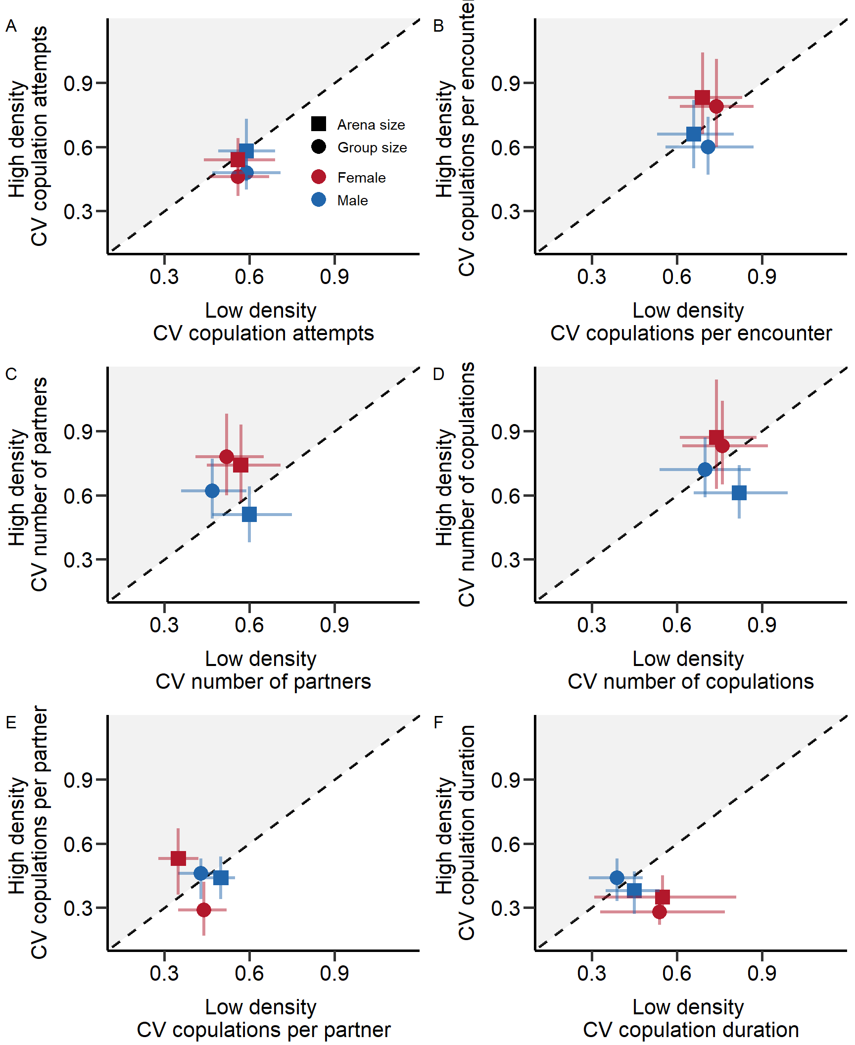
Figure S5: Coefficients of variation (CV) in mating behavior for females (blue) and males (red) under density manipulated via group (point) or arena size (square). Copulation attempts (A), proportion of successful copulations (B), number of partners (C), number of copulations (D), copulations per partners (E) and copulation duration (F) with mean and 95%CI estimated via bootstrapping (Table S2). In grey area metrics were larger under high density treatments. The x-/y-distance of means from dashed line is equal to the effect size of the treatment.
Figure_S5 = plot_grid(Figure_S5, ncol=1, rel_heights=c(0.2, 1.1)) # rel_heights values control title marginsPermutation tests for treatment comparison
Finally we tested if the coefficients of variation in mating behavior and reproductive success differed between treatments.
## Permutation tests for treatment comparison ####
### Copulation attempts ####
# Male
# Group size
Treat_diff_Male_pop_MatingA=c(Large_pop_M_MatingA_bootvar$t)-c(Small_pop_M_MatingA_bootvar$t)

t_Treat_diff_Male_pop_MatingA=mean(Treat_diff_Male_pop_MatingA,na.rm=TRUE)
t_Treat_diff_Male_pop_MatingA_lower=quantile(Treat_diff_Male_pop_MatingA,.025,na.rm=TRUE)
t_Treat_diff_Male_pop_MatingA_upper=quantile(Treat_diff_Male_pop_MatingA,.975,na.rm=TRUE)

#Permutation test to calculate p value
comb_data=c(D_data_Large_pop$m_Total_Encounters,D_data_Small_pop$m_Total_Encounters)

diff.observed = sd(na.omit((D_data_Large_pop$m_Total_Encounters)))/mean(na.omit((D_data_Large_pop$m_Total_Encounters)))-sd(na.omit((D_data_Small_pop$m_Total_Encounters)))/mean(na.omit((D_data_Small_pop$m_Total_Encounters)))

number_of_permutations = 100000
diff.random = NULL
for (i in 1 : number_of_permutations) {

  # Sample from the combined dataset
  a.random = sample (na.omit(comb_data), length(c(D_data_Large_pop$m_Total_Encounters)), TRUE)
  b.random = sample (na.omit(comb_data), length(c(D_data_Small_pop$m_Total_Encounters)), TRUE)

  # Null (permuated) difference
  diff.random[i] =  sd(na.omit(a.random))/mean(na.omit(a.random))-sd(na.omit(b.random))/mean(na.omit(b.random))
}

# P-value is the fraction of how many times the permuted difference is
# equal or more extreme than the observed difference

t_Treat_diff_Male_pop_MatingA_p = sum(abs(diff.random) >= as.numeric(abs(diff.observed)))/   number_of_permutations

# Arena
Treat_diff_Male_arena_MatingA=c(Small_arena_M_MatingA_bootvar$t)-c(Large_arena_M_MatingA_bootvar$t)

t_Treat_diff_Male_arena_MatingA=mean(Treat_diff_Male_arena_MatingA,na.rm=TRUE)
t_Treat_diff_Male_arena_MatingA_lower=quantile(Treat_diff_Male_arena_MatingA,.025,na.rm=TRUE)
t_Treat_diff_Male_arena_MatingA_upper=quantile(Treat_diff_Male_arena_MatingA,.975,na.rm=TRUE)

#Permutation test to calculate p value
comb_data=c(D_data_Large_arena$m_Total_Encounters,D_data_Small_arena$m_Total_Encounters)

diff.observed = sd(na.omit((D_data_Small_arena$m_Total_Encounters)))/mean(na.omit((D_data_Small_arena$m_Total_Encounters)))-sd(na.omit((D_data_Large_arena$m_Total_Encounters)))/mean(na.omit((D_data_Large_arena$m_Total_Encounters)))

number_of_permutations = 100000
diff.random = NULL
for (i in 1 : number_of_permutations) {

  # Sample from the combined dataset
  b.random = sample (na.omit(comb_data), length(c(D_data_Large_arena$m_Total_Encounters)), TRUE)
  a.random = sample (na.omit(comb_data), length(c(D_data_Small_arena$m_Total_Encounters)), TRUE)

  # Null (permuated) difference
  diff.random[i] =  sd(na.omit(a.random))/mean(na.omit(a.random))-sd(na.omit(b.random))/mean(na.omit(b.random))
}

# P-value is the fraction of how many times the permuted difference is
# equal or more extreme than the observed difference

t_Treat_diff_Male_arena_MatingA_p = sum(abs(diff.random) >= as.numeric(abs(diff.observed)))/   number_of_permutations

# Female
# Group size
Treat_diff_Female_pop_MatingA=c(Large_pop_F_MatingA_bootvar$t)-c(Small_pop_F_MatingA_bootvar$t)

t_Treat_diff_Female_pop_MatingA=mean(Treat_diff_Female_pop_MatingA,na.rm=TRUE)
t_Treat_diff_Female_pop_MatingA_lower=quantile(Treat_diff_Female_pop_MatingA,.025,na.rm=TRUE)
t_Treat_diff_Female_pop_MatingA_upper=quantile(Treat_diff_Female_pop_MatingA,.975,na.rm=TRUE)

#Permutation test to calculate p value
comb_data=c(D_data_Large_pop$f_Total_Encounters,D_data_Small_pop$f_Total_Encounters)

diff.observed = sd(na.omit((D_data_Large_pop$f_Total_Encounters)))/mean(na.omit((D_data_Large_pop$f_Total_Encounters)))- sd(na.omit((D_data_Small_pop$f_Total_Encounters)))/mean(na.omit((D_data_Small_pop$f_Total_Encounters)))

number_of_permutations = 100000
diff.random = NULL
for (i in 1 : number_of_permutations) {

  # Sample from the combined dataset
  a.random = sample (na.omit(comb_data), length(c(D_data_Large_pop$f_Total_Encounters)), TRUE)
  b.random = sample (na.omit(comb_data), length(c(D_data_Small_pop$f_Total_Encounters)), TRUE)

  # Null (permuated) difference
  diff.random[i] =  sd(na.omit(a.random))/mean(na.omit(a.random))-sd(na.omit(b.random))/mean(na.omit(b.random))
}

# P-value is the fraction of how many times the permuted difference is
# equal or more extreme than the observed difference

t_Treat_diff_Female_pop_MatingA_p = sum(abs(diff.random) >= as.numeric(abs(diff.observed)))/   number_of_permutations

# Arena
Treat_diff_Female_arena_MatingA=c(Small_arena_F_MatingA_bootvar$t)-c(Large_arena_F_MatingA_bootvar$t)

t_Treat_diff_Female_arena_MatingA=mean(Treat_diff_Female_arena_MatingA,na.rm=TRUE)
t_Treat_diff_Female_arena_MatingA_lower=quantile(Treat_diff_Female_arena_MatingA,.025,na.rm=TRUE)
t_Treat_diff_Female_arena_MatingA_upper=quantile(Treat_diff_Female_arena_MatingA,.975,na.rm=TRUE)

#Permutation test to calculate p value
comb_data=c(D_data_Large_arena$f_Total_Encounters,D_data_Small_arena$f_Total_Encounters)

diff.observed = sd(na.omit((D_data_Small_arena$f_Total_Encounters)))/mean(na.omit((D_data_Small_arena$f_Total_Encounters)))-sd(na.omit((D_data_Large_arena$f_Total_Encounters)))/mean(na.omit((D_data_Large_arena$f_Total_Encounters)))

number_of_permutations = 100000
diff.random = NULL
for (i in 1 : number_of_permutations) {

  # Sample from the combined dataset
  b.random = sample (na.omit(comb_data), length(c(D_data_Large_arena$f_Total_Encounters)), TRUE)
  a.random = sample (na.omit(comb_data), length(c(D_data_Small_arena$f_Total_Encounters)), TRUE)

  # Null (permuated) difference
  diff.random[i] =  sd(na.omit(a.random))/mean(na.omit(a.random))-sd(na.omit(b.random))/mean(na.omit(b.random))
}

# P-value is the fraction of how many times the permuted difference is
# equal or more extreme than the observed difference

t_Treat_diff_Female_arena_MatingA_p = sum(abs(diff.random) >= as.numeric(abs(diff.observed)))/   number_of_permutations

### Copulations per encounter ####
# Male
# Group size
Treat_diff_Male_pop_PropSucCop=c(Large_pop_M_PropSucCop_bootvar$t)-c(Small_pop_M_PropSucCop_bootvar$t)

t_Treat_diff_Male_pop_PropSucCop=mean(Treat_diff_Male_pop_PropSucCop,na.rm=TRUE)
t_Treat_diff_Male_pop_PropSucCop_lower=quantile(Treat_diff_Male_pop_PropSucCop,.025,na.rm=TRUE)
t_Treat_diff_Male_pop_PropSucCop_upper=quantile(Treat_diff_Male_pop_PropSucCop,.975,na.rm=TRUE)

#Permutation test to calculate p value
comb_data=c(D_data_Large_pop$m_TotMatings/(D_data_Large_pop$m_TotMatings+D_data_Large_pop$m_Attempts_number),D_data_Small_pop$m_TotMatings/(D_data_Small_pop$m_TotMatings+D_data_Small_pop$m_Attempts_number))

diff.observed = sd(na.omit((D_data_Large_pop$m_TotMatings/(D_data_Large_pop$m_TotMatings+D_data_Large_pop$m_Attempts_number))))/mean(na.omit((D_data_Large_pop$m_TotMatings/(D_data_Large_pop$m_TotMatings+D_data_Large_pop$m_Attempts_number))))- sd(na.omit((D_data_Small_pop$m_TotMatings/(D_data_Small_pop$m_TotMatings+D_data_Small_pop$m_Attempts_number))))/mean(na.omit((D_data_Small_pop$m_TotMatings/(D_data_Small_pop$m_TotMatings+D_data_Small_pop$m_Attempts_number))))

number_of_permutations = 100000
diff.random = NULL
for (i in 1 : number_of_permutations) {

  # Sample from the combined dataset
  a.random = sample (na.omit(comb_data), length(c(D_data_Large_pop$m_TotMatings/(D_data_Large_pop$m_TotMatings+D_data_Large_pop$m_Attempts_number))), TRUE)
  b.random = sample (na.omit(comb_data), length(c(D_data_Small_pop$m_TotMatings/(D_data_Small_pop$m_TotMatings+D_data_Small_pop$m_Attempts_number))), TRUE)

  # Null (permuated) difference
  diff.random[i] =  sd(na.omit(a.random))/mean(na.omit(a.random))-sd(na.omit(b.random))/mean(na.omit(b.random))
}

# P-value is the fraction of how many times the permuted difference is
# equal or more extreme than the observed difference

t_Treat_diff_Male_pop_PropSucCop_p = sum(abs(diff.random) >= as.numeric(abs(diff.observed)))/   number_of_permutations

# Arena
Treat_diff_Male_arena_PropSucCop=c(Small_arena_M_PropSucCop_bootvar$t)-c(Large_arena_M_PropSucCop_bootvar$t)

t_Treat_diff_Male_arena_PropSucCop=mean(Treat_diff_Male_arena_PropSucCop,na.rm=TRUE)
t_Treat_diff_Male_arena_PropSucCop_lower=quantile(Treat_diff_Male_arena_PropSucCop,.025,na.rm=TRUE)
t_Treat_diff_Male_arena_PropSucCop_upper=quantile(Treat_diff_Male_arena_PropSucCop,.975,na.rm=TRUE)

#Permutation test to calculate p value
comb_data=c(D_data_Large_arena$m_TotMatings/(D_data_Large_arena$m_TotMatings+D_data_Large_arena$m_Attempts_number),D_data_Small_arena$m_TotMatings/(D_data_Small_arena$m_TotMatings+D_data_Small_arena$m_Attempts_number))

diff.observed = sd(na.omit((D_data_Small_arena$m_TotMatings/(D_data_Small_arena$m_TotMatings+D_data_Small_arena$m_Attempts_number))))/mean(na.omit((D_data_Small_arena$m_TotMatings/(D_data_Small_arena$m_TotMatings+D_data_Small_arena$m_Attempts_number))))-sd(na.omit((D_data_Large_arena$m_TotMatings/(D_data_Large_arena$m_TotMatings+D_data_Large_arena$m_Attempts_number))))/mean(na.omit((D_data_Large_arena$m_TotMatings/(D_data_Large_arena$m_TotMatings+D_data_Large_arena$m_Attempts_number))))

number_of_permutations = 100000
diff.random = NULL
for (i in 1 : number_of_permutations) {

  # Sample from the combined dataset
  b.random = sample (na.omit(comb_data), length(c(D_data_Large_arena$m_TotMatings/(D_data_Large_arena$m_TotMatings+D_data_Large_arena$m_Attempts_number))), TRUE)
  a.random = sample (na.omit(comb_data), length(c(D_data_Small_arena$m_TotMatings/(D_data_Small_arena$m_TotMatings+D_data_Small_arena$m_Attempts_number))), TRUE)

  # Null (permuated) difference
  diff.random[i] =  sd(na.omit(a.random))/mean(na.omit(a.random))-sd(na.omit(b.random))/mean(na.omit(b.random))
}

# P-value is the fraction of how many times the permuted difference is
# equal or more extreme than the observed difference

t_Treat_diff_Male_arena_PropSucCop_p = sum(abs(diff.random) >= as.numeric(abs(diff.observed)))/   number_of_permutations

# Female
# Group size
Treat_diff_Female_pop_PropSucCop=c(Large_pop_F_PropSucCop_bootvar$t)-c(Small_pop_F_PropSucCop_bootvar$t)

t_Treat_diff_Female_pop_PropSucCop=mean(Treat_diff_Female_pop_PropSucCop,na.rm=TRUE)
t_Treat_diff_Female_pop_PropSucCop_lower=quantile(Treat_diff_Female_pop_PropSucCop,.025,na.rm=TRUE)
t_Treat_diff_Female_pop_PropSucCop_upper=quantile(Treat_diff_Female_pop_PropSucCop,.975,na.rm=TRUE)

#Permutation test to calculate p value
comb_data=c(D_data_Large_pop$f_TotMatings/(D_data_Large_pop$f_TotMatings+D_data_Large_pop$f_Attempts_number),D_data_Small_pop$f_TotMatings/(D_data_Small_pop$f_TotMatings+D_data_Small_pop$f_Attempts_number))

diff.observed = sd(na.omit((D_data_Large_pop$f_TotMatings/(D_data_Large_pop$f_TotMatings+D_data_Large_pop$f_Attempts_number))))/mean(na.omit((D_data_Large_pop$f_TotMatings/(D_data_Large_pop$f_TotMatings+D_data_Large_pop$f_Attempts_number))))-sd(na.omit((D_data_Small_pop$f_TotMatings/(D_data_Small_pop$f_TotMatings+D_data_Small_pop$f_Attempts_number))))/mean(na.omit((D_data_Small_pop$f_TotMatings/(D_data_Small_pop$f_TotMatings+D_data_Small_pop$f_Attempts_number))))

number_of_permutations = 100000
diff.random = NULL
for (i in 1 : number_of_permutations) {

  # Sample from the combined dataset
  a.random = sample (na.omit(comb_data), length(c(D_data_Large_pop$f_TotMatings/(D_data_Large_pop$f_TotMatings+D_data_Large_pop$f_Attempts_number))), TRUE)
  b.random = sample (na.omit(comb_data), length(c(D_data_Small_pop$f_TotMatings/(D_data_Small_pop$f_TotMatings+D_data_Small_pop$f_Attempts_number))), TRUE)

  # Null (permuated) difference
  diff.random[i] =  sd(na.omit(a.random))/mean(na.omit(a.random))-sd(na.omit(b.random))/mean(na.omit(b.random))
}

# P-value is the fraction of how many times the permuted difference is
# equal or more extreme than the observed difference

t_Treat_diff_Female_pop_PropSucCop_p = sum(abs(diff.random) >= as.numeric(abs(diff.observed)))/   number_of_permutations

# Arena
Treat_diff_Female_arena_PropSucCop=c(Small_arena_F_PropSucCop_bootvar$t)-c(Large_arena_F_PropSucCop_bootvar$t)

t_Treat_diff_Female_arena_PropSucCop=mean(Treat_diff_Female_arena_PropSucCop,na.rm=TRUE)
t_Treat_diff_Female_arena_PropSucCop_lower=quantile(Treat_diff_Female_arena_PropSucCop,.025,na.rm=TRUE)
t_Treat_diff_Female_arena_PropSucCop_upper=quantile(Treat_diff_Female_arena_PropSucCop,.975,na.rm=TRUE)

#Permutation test to calculate p value
comb_data=c(D_data_Large_arena$f_TotMatings/(D_data_Large_arena$f_TotMatings+D_data_Large_arena$f_Attempts_number),D_data_Small_arena$f_TotMatings/(D_data_Small_arena$f_TotMatings+D_data_Small_arena$f_Attempts_number))

diff.observed = sd(na.omit((D_data_Small_arena$f_TotMatings/(D_data_Small_arena$f_TotMatings+D_data_Small_arena$f_Attempts_number))))/mean(na.omit((D_data_Small_arena$f_TotMatings/(D_data_Small_arena$f_TotMatings+D_data_Small_arena$f_Attempts_number))))-sd(na.omit((D_data_Large_arena$f_TotMatings/(D_data_Large_arena$f_TotMatings+D_data_Large_arena$f_Attempts_number))))/mean(na.omit((D_data_Large_arena$f_TotMatings/(D_data_Large_arena$f_TotMatings+D_data_Large_arena$f_Attempts_number))))

number_of_permutations = 100000
diff.random = NULL
for (i in 1 : number_of_permutations) {

  # Sample from the combined dataset
  b.random = sample (na.omit(comb_data), length(c(D_data_Large_arena$f_TotMatings/(D_data_Large_arena$f_TotMatings+D_data_Large_arena$f_Attempts_number))), TRUE)
  a.random = sample (na.omit(comb_data), length(c(D_data_Small_arena$f_TotMatings/(D_data_Small_arena$f_TotMatings+D_data_Small_arena$f_Attempts_number))), TRUE)

  # Null (permuated) difference
  diff.random[i] =  sd(na.omit(a.random))/mean(na.omit(a.random))-sd(na.omit(b.random))/mean(na.omit(b.random))
}

# P-value is the fraction of how many times the permuted difference is
# equal or more extreme than the observed difference

t_Treat_diff_Female_arena_PropSucCop_p = sum(abs(diff.random) >= as.numeric(abs(diff.observed)))/   number_of_permutations

### Number of partners ####
# Male
# Group size
Treat_diff_Male_pop_MS=c(Large_pop_M_MS_bootvar$t)-c(Small_pop_M_MS_bootvar$t)

t_Treat_diff_Male_pop_MS=mean(Treat_diff_Male_pop_MS,na.rm=TRUE)
t_Treat_diff_Male_pop_MS_lower=quantile(Treat_diff_Male_pop_MS,.025,na.rm=TRUE)
t_Treat_diff_Male_pop_MS_upper=quantile(Treat_diff_Male_pop_MS,.975,na.rm=TRUE)

#Permutation test to calculate p value
comb_data=c(D_data_Large_pop$m_cMS,D_data_Small_pop$m_cMS)

diff.observed = sd(na.omit((D_data_Large_pop$m_cMS)))/mean(na.omit((D_data_Large_pop$m_cMS))) -sd(na.omit((D_data_Small_pop$m_cMS)))/mean(na.omit((D_data_Small_pop$m_cMS)))

number_of_permutations = 100000
diff.random = NULL
for (i in 1 : number_of_permutations) {

  # Sample from the combined dataset
  a.random = sample (na.omit(comb_data), length(c(D_data_Large_pop$m_cMS)), TRUE)
  b.random = sample (na.omit(comb_data), length(c(D_data_Small_pop$m_cMS)), TRUE)

  # Null (permuated) difference
  diff.random[i] =  sd(na.omit(a.random))/mean(na.omit(a.random))-sd(na.omit(b.random))/mean(na.omit(b.random))
}

# P-value is the fraction of how many times the permuted difference is
# equal or more extreme than the observed difference

t_Treat_diff_Male_pop_MS_p = sum(abs(diff.random) >= as.numeric(abs(diff.observed)))/   number_of_permutations

# Arena
Treat_diff_Male_arena_MS=c(Small_arena_M_MS_bootvar$t)-c(Large_arena_M_MS_bootvar$t)

t_Treat_diff_Male_arena_MS=mean(Treat_diff_Male_arena_MS,na.rm=TRUE)
t_Treat_diff_Male_arena_MS_lower=quantile(Treat_diff_Male_arena_MS,.025,na.rm=TRUE)
t_Treat_diff_Male_arena_MS_upper=quantile(Treat_diff_Male_arena_MS,.975,na.rm=TRUE)

#Permutation test to calculate p value
comb_data=c(D_data_Large_arena$m_cMS,D_data_Small_arena$m_cMS)

diff.observed = sd(na.omit((D_data_Small_arena$m_cMS)))/mean(na.omit((D_data_Small_arena$m_cMS)))-sd(na.omit((D_data_Large_arena$m_cMS)))/mean(na.omit((D_data_Large_arena$m_cMS)))

number_of_permutations = 100000
diff.random = NULL
for (i in 1 : number_of_permutations) {

  # Sample from the combined dataset
  b.random = sample (na.omit(comb_data), length(c(D_data_Large_arena$m_cMS)), TRUE)
  a.random = sample (na.omit(comb_data), length(c(D_data_Small_arena$m_cMS)), TRUE)

  # Null (permuated) difference
  diff.random[i] =  sd(na.omit(a.random))/mean(na.omit(a.random))-sd(na.omit(b.random))/mean(na.omit(b.random))
}

# P-value is the fraction of how many times the permuted difference is
# equal or more extreme than the observed difference

t_Treat_diff_Male_arena_MS_p = sum(abs(diff.random) >= as.numeric(abs(diff.observed)))/   number_of_permutations

# Female
# Group size
Treat_diff_Female_pop_MS=c(Large_pop_F_MS_bootvar$t)-c(Small_pop_F_MS_bootvar$t)

t_Treat_diff_Female_pop_MS=mean(Treat_diff_Female_pop_MS,na.rm=TRUE)
t_Treat_diff_Female_pop_MS_lower=quantile(Treat_diff_Female_pop_MS,.025,na.rm=TRUE)
t_Treat_diff_Female_pop_MS_upper=quantile(Treat_diff_Female_pop_MS,.975,na.rm=TRUE)

#Permutation test to calculate p value
comb_data=c(D_data_Large_pop$m_cMS,D_data_Small_pop$m_cMS)

diff.observed = sd(na.omit((D_data_Large_pop$m_cMS)))/mean(na.omit((D_data_Large_pop$m_cMS)))-sd(na.omit((D_data_Small_pop$m_cMS)))/mean(na.omit((D_data_Small_pop$m_cMS)))

number_of_permutations = 100000
diff.random = NULL
for (i in 1 : number_of_permutations) {

  # Sample from the combined dataset
  a.random = sample (na.omit(comb_data), length(c(D_data_Large_pop$m_cMS)), TRUE)
  b.random = sample (na.omit(comb_data), length(c(D_data_Small_pop$m_cMS)), TRUE)

  # Null (permuated) difference
  diff.random[i] =  sd(na.omit(a.random))/mean(na.omit(a.random))-sd(na.omit(b.random))/mean(na.omit(b.random))
}

# P-value is the fraction of how many times the permuted difference is
# equal or more extreme than the observed difference

t_Treat_diff_Female_pop_MS_p = sum(abs(diff.random) >= as.numeric(abs(diff.observed)))/   number_of_permutations

# Arena
Treat_diff_Female_arena_MS=c(Small_arena_F_MS_bootvar$t)-c(Large_arena_F_MS_bootvar$t)

t_Treat_diff_Female_arena_MS=mean(Treat_diff_Female_arena_MS,na.rm=TRUE)
t_Treat_diff_Female_arena_MS_lower=quantile(Treat_diff_Female_arena_MS,.025,na.rm=TRUE)
t_Treat_diff_Female_arena_MS_upper=quantile(Treat_diff_Female_arena_MS,.975,na.rm=TRUE)

#Permutation test to calculate p value
comb_data=c(D_data_Large_arena$m_cMS,D_data_Small_arena$m_cMS)

diff.observed = sd(na.omit((D_data_Small_arena$m_cMS)))/mean(na.omit((D_data_Small_arena$m_cMS)))-sd(na.omit((D_data_Large_arena$m_cMS)))/mean(na.omit((D_data_Large_arena$m_cMS)))

number_of_permutations = 100000
diff.random = NULL
for (i in 1 : number_of_permutations) {

  # Sample from the combined dataset
  b.random = sample (na.omit(comb_data), length(c(D_data_Large_arena$m_cMS)), TRUE)
  a.random = sample (na.omit(comb_data), length(c(D_data_Small_arena$m_cMS)), TRUE)

  # Null (permuated) difference
  diff.random[i] =  sd(na.omit(a.random))/mean(na.omit(a.random))-sd(na.omit(b.random))/mean(na.omit(b.random))
}

# P-value is the fraction of how many times the permuted difference is
# equal or more extreme than the observed difference

t_Treat_diff_Female_arena_MS_p = sum(abs(diff.random) >= as.numeric(abs(diff.observed)))/   number_of_permutations

### Number of copulations ####
# Male
# Group size
Treat_diff_Male_pop_Matings=c(Large_pop_M_Matings_bootvar$t)-c(Small_pop_M_Matings_bootvar$t)

t_Treat_diff_Male_pop_Matings=mean(Treat_diff_Male_pop_Matings,na.rm=TRUE)
t_Treat_diff_Male_pop_Matings_lower=quantile(Treat_diff_Male_pop_Matings,.025,na.rm=TRUE)
t_Treat_diff_Male_pop_Matings_upper=quantile(Treat_diff_Male_pop_Matings,.975,na.rm=TRUE)

#Permutation test to calculate p value
comb_data=c(D_data_Large_pop$m_TotMatings,D_data_Small_pop$m_TotMatings)

diff.observed = sd(na.omit((D_data_Large_pop$m_TotMatings)))/mean(na.omit((D_data_Large_pop$m_TotMatings))) -sd(na.omit((D_data_Small_pop$m_TotMatings)))/mean(na.omit((D_data_Small_pop$m_TotMatings)))

number_of_permutations = 100000
diff.random = NULL
for (i in 1 : number_of_permutations) {

  # Sample from the combined dataset
  a.random = sample (na.omit(comb_data), length(c(D_data_Large_pop$m_TotMatings)), TRUE)
  b.random = sample (na.omit(comb_data), length(c(D_data_Small_pop$m_TotMatings)), TRUE)

  # Null (permuated) difference
  diff.random[i] =  sd(na.omit(a.random))/mean(na.omit(a.random))-sd(na.omit(b.random))/mean(na.omit(b.random))
}

# P-value is the fraction of how many times the permuted difference is
# equal or more extreme than the observed difference

t_Treat_diff_Male_pop_Matings_p = sum(abs(diff.random) >= as.numeric(abs(diff.observed)))/   number_of_permutations

# Arena
Treat_diff_Male_arena_Matings=c(Small_arena_M_Matings_bootvar$t)-c(Large_arena_M_Matings_bootvar$t)

t_Treat_diff_Male_arena_Matings=mean(Treat_diff_Male_arena_Matings,na.rm=TRUE)
t_Treat_diff_Male_arena_Matings_lower=quantile(Treat_diff_Male_arena_Matings,.025,na.rm=TRUE)
t_Treat_diff_Male_arena_Matings_upper=quantile(Treat_diff_Male_arena_Matings,.975,na.rm=TRUE)

#Permutation test to calculate p value
comb_data=c(D_data_Large_arena$m_TotMatings,D_data_Small_arena$m_TotMatings)

diff.observed = sd(na.omit((D_data_Small_arena$m_TotMatings)))/mean(na.omit((D_data_Small_arena$m_TotMatings)))-sd(na.omit((D_data_Large_arena$m_TotMatings)))/mean(na.omit((D_data_Large_arena$m_TotMatings)))

number_of_permutations = 100000
diff.random = NULL
for (i in 1 : number_of_permutations) {

  # Sample from the combined dataset
  b.random = sample (na.omit(comb_data), length(c(D_data_Large_arena$m_TotMatings)), TRUE)
  a.random = sample (na.omit(comb_data), length(c(D_data_Small_arena$m_TotMatings)), TRUE)

  # Null (permuated) difference
  diff.random[i] =  sd(na.omit(a.random))/mean(na.omit(a.random))-sd(na.omit(b.random))/mean(na.omit(b.random))
}

# P-value is the fraction of how many times the permuted difference is
# equal or more extreme than the observed difference

t_Treat_diff_Male_arena_Matings_p = sum(abs(diff.random) >= as.numeric(abs(diff.observed)))/   number_of_permutations

# Female
# Group size
Treat_diff_Female_pop_Matings=c(Large_pop_F_Matings_bootvar$t)-c(Small_pop_F_Matings_bootvar$t)

t_Treat_diff_Female_pop_Matings=mean(Treat_diff_Female_pop_Matings,na.rm=TRUE)
t_Treat_diff_Female_pop_Matings_lower=quantile(Treat_diff_Female_pop_Matings,.025,na.rm=TRUE)
t_Treat_diff_Female_pop_Matings_upper=quantile(Treat_diff_Female_pop_Matings,.975,na.rm=TRUE)

#Permutation test to calculate p value
comb_data=c(D_data_Large_pop$f_TotMatings,D_data_Small_pop$f_TotMatings)

diff.observed = sd(na.omit((D_data_Large_pop$f_TotMatings)))/mean(na.omit((D_data_Large_pop$f_TotMatings)))-sd(na.omit((D_data_Small_pop$f_TotMatings)))/mean(na.omit((D_data_Small_pop$f_TotMatings)))

number_of_permutations = 100000
diff.random = NULL
for (i in 1 : number_of_permutations) {

  # Sample from the combined dataset
  a.random = sample (na.omit(comb_data), length(c(D_data_Large_pop$f_TotMatings)), TRUE)
  b.random = sample (na.omit(comb_data), length(c(D_data_Small_pop$f_TotMatings)), TRUE)

  # Null (permuated) difference
  diff.random[i] =  sd(na.omit(a.random))/mean(na.omit(a.random))-sd(na.omit(b.random))/mean(na.omit(b.random))
}

# P-value is the fraction of how many times the permuted difference is
# equal or more extreme than the observed difference

t_Treat_diff_Female_pop_Matings_p = sum(abs(diff.random) >= as.numeric(abs(diff.observed)))/   number_of_permutations

# Arena
Treat_diff_Female_arena_Matings=c(Small_arena_F_Matings_bootvar$t)-c(Large_arena_F_Matings_bootvar$t)

t_Treat_diff_Female_arena_Matings=mean(Treat_diff_Female_arena_Matings,na.rm=TRUE)
t_Treat_diff_Female_arena_Matings_lower=quantile(Treat_diff_Female_arena_Matings,.025,na.rm=TRUE)
t_Treat_diff_Female_arena_Matings_upper=quantile(Treat_diff_Female_arena_Matings,.975,na.rm=TRUE)

#Permutation test to calculate p value
comb_data=c(D_data_Large_arena$f_TotMatings,D_data_Small_arena$f_TotMatings)

diff.observed = sd(na.omit((D_data_Small_arena$f_TotMatings)))/mean(na.omit((D_data_Small_arena$f_TotMatings)))-sd(na.omit((D_data_Large_arena$f_TotMatings)))/mean(na.omit((D_data_Large_arena$f_TotMatings)))

number_of_permutations = 100000
diff.random = NULL
for (i in 1 : number_of_permutations) {

  # Sample from the combined dataset
  b.random = sample (na.omit(comb_data), length(c(D_data_Large_arena$f_TotMatings)), TRUE)
  a.random = sample (na.omit(comb_data), length(c(D_data_Small_arena$f_TotMatings)), TRUE)

  # Null (permuated) difference
  diff.random[i] =  sd(na.omit(a.random))/mean(na.omit(a.random))-sd(na.omit(b.random))/mean(na.omit(b.random))
}

# P-value is the fraction of how many times the permuted difference is
# equal or more extreme than the observed difference

t_Treat_diff_Female_arena_Matings_p = sum(abs(diff.random) >= as.numeric(abs(diff.observed)))/   number_of_permutations

### Copulations per partner ####
# Male
# Group size
Treat_diff_Male_pop_MeanCop=c(Large_pop_M_MeanCop_bootvar$t)-c(Small_pop_M_MeanCop_bootvar$t)

t_Treat_diff_Male_pop_MeanCop=mean(Treat_diff_Male_pop_MeanCop,na.rm=TRUE)
t_Treat_diff_Male_pop_MeanCop_lower=quantile(Treat_diff_Male_pop_MeanCop,.025,na.rm=TRUE)
t_Treat_diff_Male_pop_MeanCop_upper=quantile(Treat_diff_Male_pop_MeanCop,.975,na.rm=TRUE)

#Permutation test to calculate p value
comb_data=c(D_data_Large_pop$m_meanCop,D_data_Small_pop$m_meanCop)

diff.observed =sd(na.omit((D_data_Large_pop$m_meanCop)))/mean(na.omit((D_data_Large_pop$m_meanCop))) - sd(na.omit((D_data_Small_pop$m_meanCop)))/mean(na.omit((D_data_Small_pop$m_meanCop)))

number_of_permutations = 100000
diff.random = NULL
for (i in 1 : number_of_permutations) {

  # Sample from the combined dataset
  a.random = sample (na.omit(comb_data), length(c(D_data_Large_pop$m_meanCop)), TRUE)
  b.random = sample (na.omit(comb_data), length(c(D_data_Small_pop$m_meanCop)), TRUE)

  # Null (permuated) difference
  diff.random[i] =  sd(na.omit(a.random))/mean(na.omit(a.random))-sd(na.omit(b.random))/mean(na.omit(b.random))
}

# P-value is the fraction of how many times the permuted difference is
# equal or more extreme than the observed difference

t_Treat_diff_Male_pop_MeanCop_p = sum(abs(diff.random) >= as.numeric(abs(diff.observed)))/   number_of_permutations

# Arena
Treat_diff_Male_arena_MeanCop=c(Small_arena_M_MeanCop_bootvar$t)-c(Large_arena_M_MeanCop_bootvar$t)

t_Treat_diff_Male_arena_MeanCop=mean(Treat_diff_Male_arena_MeanCop,na.rm=TRUE)
t_Treat_diff_Male_arena_MeanCop_lower=quantile(Treat_diff_Male_arena_MeanCop,.025,na.rm=TRUE)
t_Treat_diff_Male_arena_MeanCop_upper=quantile(Treat_diff_Male_arena_MeanCop,.975,na.rm=TRUE)

#Permutation test to calculate p value
comb_data=c(D_data_Large_arena$m_meanCop,D_data_Small_arena$m_meanCop)

diff.observed = sd(na.omit((D_data_Small_arena$m_meanCop)))/mean(na.omit((D_data_Small_arena$m_meanCop)))-sd(na.omit((D_data_Large_arena$m_meanCop)))/mean(na.omit((D_data_Large_arena$m_meanCop)))

number_of_permutations = 100000
diff.random = NULL
for (i in 1 : number_of_permutations) {

  # Sample from the combined dataset
  b.random = sample (na.omit(comb_data), length(c(D_data_Large_arena$m_meanCop)), TRUE)
  a.random = sample (na.omit(comb_data), length(c(D_data_Small_arena$m_meanCop)), TRUE)

  # Null (permuated) difference
  diff.random[i] =  sd(na.omit(a.random))/mean(na.omit(a.random))-sd(na.omit(b.random))/mean(na.omit(b.random))
}

# P-value is the fraction of how many times the permuted difference is
# equal or more extreme than the observed difference

t_Treat_diff_Male_arena_MeanCop_p = sum(abs(diff.random) >= as.numeric(abs(diff.observed)))/   number_of_permutations

# Female
# Group size
Treat_diff_Female_pop_MeanCop=c(Large_pop_F_MeanCop_bootvar$t)-c(Small_pop_F_MeanCop_bootvar$t)

t_Treat_diff_Female_pop_MeanCop=mean(Treat_diff_Female_pop_MeanCop,na.rm=TRUE)
t_Treat_diff_Female_pop_MeanCop_lower=quantile(Treat_diff_Female_pop_MeanCop,.025,na.rm=TRUE)
t_Treat_diff_Female_pop_MeanCop_upper=quantile(Treat_diff_Female_pop_MeanCop,.975,na.rm=TRUE)

#Permutation test to calculate p value
comb_data=c(D_data_Large_pop$f_meanCop,D_data_Small_pop$f_meanCop)

diff.observed =sd(na.omit((D_data_Large_pop$f_meanCop)))/mean(na.omit((D_data_Large_pop$f_meanCop))) -sd(na.omit((D_data_Small_pop$f_meanCop)))/mean(na.omit((D_data_Small_pop$f_meanCop)))

number_of_permutations = 100000
diff.random = NULL
for (i in 1 : number_of_permutations) {

  # Sample from the combined dataset
  a.random = sample (na.omit(comb_data), length(c(D_data_Large_pop$f_meanCop)), TRUE)
  b.random = sample (na.omit(comb_data), length(c(D_data_Small_pop$f_meanCop)), TRUE)

  # Null (permuated) difference
  diff.random[i] =  sd(na.omit(a.random))/mean(na.omit(a.random))-sd(na.omit(b.random))/mean(na.omit(b.random))
}

# P-value is the fraction of how many times the permuted difference is
# equal or more extreme than the observed difference

t_Treat_diff_Female_pop_MeanCop_p = sum(abs(diff.random) >= as.numeric(abs(diff.observed)))/   number_of_permutations

# Arena
Treat_diff_Female_arena_MeanCop=c(Small_arena_F_MeanCop_bootvar$t)-c(Large_arena_F_MeanCop_bootvar$t)

t_Treat_diff_Female_arena_MeanCop=mean(Treat_diff_Female_arena_MeanCop,na.rm=TRUE)
t_Treat_diff_Female_arena_MeanCop_lower=quantile(Treat_diff_Female_arena_MeanCop,.025,na.rm=TRUE)
t_Treat_diff_Female_arena_MeanCop_upper=quantile(Treat_diff_Female_arena_MeanCop,.975,na.rm=TRUE)

#Permutation test to calculate p value
comb_data=c(D_data_Large_arena$f_meanCop,D_data_Small_arena$f_meanCop)

diff.observed = sd(na.omit((D_data_Small_arena$f_meanCop)))/mean(na.omit((D_data_Small_arena$f_meanCop)))-sd(na.omit((D_data_Large_arena$f_meanCop)))/mean(na.omit((D_data_Large_arena$f_meanCop)))

number_of_permutations = 100000
diff.random = NULL
for (i in 1 : number_of_permutations) {

  # Sample from the combined dataset
  b.random = sample (na.omit(comb_data), length(c(D_data_Large_arena$f_meanCop)), TRUE)
  a.random = sample (na.omit(comb_data), length(c(D_data_Small_arena$f_meanCop)), TRUE)

  # Null (permuated) difference
  diff.random[i] =  sd(na.omit(a.random))/mean(na.omit(a.random))-sd(na.omit(b.random))/mean(na.omit(b.random))
}

# P-value is the fraction of how many times the permuted difference is
# equal or more extreme than the observed difference

t_Treat_diff_Female_arena_MeanCop_p = sum(abs(diff.random) >= as.numeric(abs(diff.observed)))/   number_of_permutations

### Mating duration ####
# Male
# Group size
Treat_diff_Male_pop_Duration=c(Large_pop_M_Duration_bootvar$t)-c(Small_pop_M_Duration_bootvar$t)

t_Treat_diff_Male_pop_Duration=mean(Treat_diff_Male_pop_Duration,na.rm=TRUE)
t_Treat_diff_Male_pop_Duration_lower=quantile(Treat_diff_Male_pop_Duration,.025,na.rm=TRUE)
t_Treat_diff_Male_pop_Duration_upper=quantile(Treat_diff_Male_pop_Duration,.975,na.rm=TRUE)

#Permutation test to calculate p value
comb_data=c(D_data_Large_pop$m_MatingDuration_av,D_data_Small_pop$m_MatingDuration_av)

diff.observed = sd(na.omit((D_data_Large_pop$m_MatingDuration_av)))/mean(na.omit((D_data_Large_pop$m_MatingDuration_av)))- sd(na.omit((D_data_Small_pop$m_MatingDuration_av)))/mean(na.omit((D_data_Small_pop$m_MatingDuration_av)))

number_of_permutations = 100000
diff.random = NULL
for (i in 1 : number_of_permutations) {

  # Sample from the combined dataset
  a.random = sample (na.omit(comb_data), length(c(D_data_Large_pop$m_MatingDuration_av)), TRUE)
  b.random = sample (na.omit(comb_data), length(c(D_data_Small_pop$m_MatingDuration_av)), TRUE)

  # Null (permuated) difference
  diff.random[i] =  sd(na.omit(a.random))/mean(na.omit(a.random))-sd(na.omit(b.random))/mean(na.omit(b.random))
}

# P-value is the fraction of how many times the permuted difference is
# equal or more extreme than the observed difference

t_Treat_diff_Male_pop_Duration_p = sum(abs(diff.random) >= as.numeric(abs(diff.observed)))/   number_of_permutations

# Arena
Treat_diff_Male_arena_Duration=c(Small_arena_M_Duration_bootvar$t)-c(Large_arena_M_Duration_bootvar$t)

t_Treat_diff_Male_arena_Duration=mean(Treat_diff_Male_arena_Duration,na.rm=TRUE)
t_Treat_diff_Male_arena_Duration_lower=quantile(Treat_diff_Male_arena_Duration,.025,na.rm=TRUE)
t_Treat_diff_Male_arena_Duration_upper=quantile(Treat_diff_Male_arena_Duration,.975,na.rm=TRUE)

#Permutation test to calculate p value
comb_data=c(D_data_Large_arena$m_MatingDuration_av,D_data_Small_arena$m_MatingDuration_av)

diff.observed = sd(na.omit((D_data_Small_arena$m_MatingDuration_av)))/mean(na.omit((D_data_Small_arena$m_MatingDuration_av)))-sd(na.omit((D_data_Large_arena$m_MatingDuration_av)))/mean(na.omit((D_data_Large_arena$m_MatingDuration_av)))

number_of_permutations = 100000
diff.random = NULL
for (i in 1 : number_of_permutations) {

  # Sample from the combined dataset
  b.random = sample (na.omit(comb_data), length(c(D_data_Large_arena$m_MatingDuration_av)), TRUE)
  a.random = sample (na.omit(comb_data), length(c(D_data_Small_arena$m_MatingDuration_av)), TRUE)

  # Null (permuated) difference
  diff.random[i] =  sd(na.omit(a.random))/mean(na.omit(a.random))-sd(na.omit(b.random))/mean(na.omit(b.random))
}

# P-value is the fraction of how many times the permuted difference is
# equal or more extreme than the observed difference

t_Treat_diff_Male_arena_Duration_p = sum(abs(diff.random) >= as.numeric(abs(diff.observed)))/   number_of_permutations

# Female
# Group size
Treat_diff_Female_pop_Duration=c(Large_pop_F_Duration_bootvar$t)-c(Small_pop_F_Duration_bootvar$t)

t_Treat_diff_Female_pop_Duration=mean(Treat_diff_Female_pop_Duration,na.rm=TRUE)
t_Treat_diff_Female_pop_Duration_lower=quantile(Treat_diff_Female_pop_Duration,.025,na.rm=TRUE)
t_Treat_diff_Female_pop_Duration_upper=quantile(Treat_diff_Female_pop_Duration,.975,na.rm=TRUE)

#Permutation test to calculate p value
comb_data=c(D_data_Large_pop$f_MatingDuration_av,D_data_Small_pop$f_MatingDuration_av)

diff.observed = sd(na.omit((D_data_Large_pop$f_MatingDuration_av)))/mean(na.omit((D_data_Large_pop$f_MatingDuration_av)))-sd(na.omit((D_data_Small_pop$f_MatingDuration_av)))/mean(na.omit((D_data_Small_pop$f_MatingDuration_av)))

number_of_permutations = 100000
diff.random = NULL
for (i in 1 : number_of_permutations) {

  # Sample from the combined dataset
  a.random = sample (na.omit(comb_data), length(c(D_data_Large_pop$f_MatingDuration_av)), TRUE)
  b.random = sample (na.omit(comb_data), length(c(D_data_Small_pop$f_MatingDuration_av)), TRUE)

  # Null (permuated) difference
  diff.random[i] =  sd(na.omit(a.random))/mean(na.omit(a.random))-sd(na.omit(b.random))/mean(na.omit(b.random))
}

# P-value is the fraction of how many times the permuted difference is
# equal or more extreme than the observed difference

t_Treat_diff_Female_pop_Duration_p = sum(abs(diff.random) >= as.numeric(abs(diff.observed)))/   number_of_permutations

# Arena
Treat_diff_Female_arena_Duration=c(Small_arena_F_Duration_bootvar$t)-c(Large_arena_F_Duration_bootvar$t)

t_Treat_diff_Female_arena_Duration=mean(Treat_diff_Female_arena_Duration,na.rm=TRUE)
t_Treat_diff_Female_arena_Duration_lower=quantile(Treat_diff_Female_arena_Duration,.025,na.rm=TRUE)
t_Treat_diff_Female_arena_Duration_upper=quantile(Treat_diff_Female_arena_Duration,.975,na.rm=TRUE)

#Permutation test to calculate p value
comb_data=c(D_data_Large_arena$f_MatingDuration_av,D_data_Small_arena$f_MatingDuration_av)

diff.observed = sd(na.omit((D_data_Small_arena$f_MatingDuration_av)))/mean(na.omit((D_data_Small_arena$f_MatingDuration_av)))-sd(na.omit((D_data_Large_arena$f_MatingDuration_av)))/mean(na.omit((D_data_Large_arena$f_MatingDuration_av)))

number_of_permutations = 100000
diff.random = NULL
for (i in 1 : number_of_permutations) {

  # Sample from the combined dataset
  b.random = sample (na.omit(comb_data), length(c(D_data_Large_arena$f_MatingDuration_av)), TRUE)
  a.random = sample (na.omit(comb_data), length(c(D_data_Small_arena$f_MatingDuration_av)), TRUE)

  # Null (permuated) difference
  diff.random[i] =  sd(na.omit(a.random))/mean(na.omit(a.random))-sd(na.omit(b.random))/mean(na.omit(b.random))
}

# P-value is the fraction of how many times the permuted difference is
# equal or more extreme than the observed difference

t_Treat_diff_Female_arena_Duration_p = sum(abs(diff.random) >= as.numeric(abs(diff.observed)))/   number_of_permutations

### Extract data and write results table ####
CompTreat_Table_Male_pop_MatingA <- as.data.frame(cbind("Male", "Group size", "Copulation attempts", t_Treat_diff_Male_pop_MatingA, t_Treat_diff_Male_pop_MatingA_lower, t_Treat_diff_Male_pop_MatingA_upper, t_Treat_diff_Male_pop_MatingA_p))
names(CompTreat_Table_Male_pop_MatingA)=c('V1','V2','V3','V4','V5','V6','V7')
CompTreat_Table_Female_pop_MatingA <- as.data.frame(cbind("Female", "Group size", "Copulation attempts", t_Treat_diff_Female_pop_MatingA, t_Treat_diff_Female_pop_MatingA_lower, t_Treat_diff_Female_pop_MatingA_upper, t_Treat_diff_Female_pop_MatingA_p))
names(CompTreat_Table_Female_pop_MatingA)=c('V1','V2','V3','V4','V5','V6','V7')
CompTreat_Table_Male_pop_PropSucCop <- as.data.frame(cbind("Male", "Group size", "Copulations per encounter", t_Treat_diff_Male_pop_PropSucCop, t_Treat_diff_Male_pop_PropSucCop_lower, t_Treat_diff_Male_pop_PropSucCop_upper, t_Treat_diff_Male_pop_PropSucCop_p))
names(CompTreat_Table_Male_pop_PropSucCop)=c('V1','V2','V3','V4','V5','V6','V7')
CompTreat_Table_Female_pop_PropSucCop <- as.data.frame(cbind("Female", "Group size", "Copulations per encounter", t_Treat_diff_Female_pop_PropSucCop, t_Treat_diff_Female_pop_PropSucCop_lower, t_Treat_diff_Female_pop_PropSucCop_upper, t_Treat_diff_Female_pop_PropSucCop_p))
names(CompTreat_Table_Female_pop_PropSucCop)=c('V1','V2','V3','V4','V5','V6','V7')
CompTreat_Table_Male_pop_Matings <- as.data.frame(cbind("Male", "Group size", "Number of copulations", t_Treat_diff_Male_pop_Matings, t_Treat_diff_Male_pop_Matings_lower, t_Treat_diff_Male_pop_Matings_upper, t_Treat_diff_Male_pop_Matings_p))
names(CompTreat_Table_Male_pop_Matings)=c('V1','V2','V3','V4','V5','V6','V7')
CompTreat_Table_Female_pop_Matings <- as.data.frame(cbind("Female", "Group size", "Number of copulations", t_Treat_diff_Female_pop_Matings, t_Treat_diff_Female_pop_Matings_lower, t_Treat_diff_Female_pop_Matings_upper, t_Treat_diff_Female_pop_Matings_p))
names(CompTreat_Table_Female_pop_Matings)=c('V1','V2','V3','V4','V5','V6','V7')
CompTreat_Table_Male_pop_MeanCop <- as.data.frame(cbind("Male", "Group size", "Copulations per partner", t_Treat_diff_Male_pop_MeanCop, t_Treat_diff_Male_pop_MeanCop_lower, t_Treat_diff_Male_pop_MeanCop_upper, t_Treat_diff_Male_pop_MeanCop_p))
names(CompTreat_Table_Male_pop_MeanCop)=c('V1','V2','V3','V4','V5','V6','V7')
CompTreat_Table_Female_pop_MeanCop <- as.data.frame(cbind("Female", "Group size", "Copulations per partner", t_Treat_diff_Female_pop_MeanCop, t_Treat_diff_Female_pop_MeanCop_lower, t_Treat_diff_Female_pop_MeanCop_upper, t_Treat_diff_Female_pop_MeanCop_p))
names(CompTreat_Table_Female_pop_MeanCop)=c('V1','V2','V3','V4','V5','V6','V7')
CompTreat_Table_Male_pop_Duration <- as.data.frame(cbind("Male", "Group size", "Mating duration", t_Treat_diff_Male_pop_Duration, t_Treat_diff_Male_pop_Duration_lower, t_Treat_diff_Male_pop_Duration_upper, t_Treat_diff_Male_pop_Duration_p))
names(CompTreat_Table_Male_pop_Duration)=c('V1','V2','V3','V4','V5','V6','V7')
CompTreat_Table_Female_pop_Duration <- as.data.frame(cbind("Female", "Group size", "Mating duration", t_Treat_diff_Female_pop_Duration, t_Treat_diff_Female_pop_Duration_lower, t_Treat_diff_Female_pop_Duration_upper, t_Treat_diff_Female_pop_Duration_p))
names(CompTreat_Table_Female_pop_Duration)=c('V1','V2','V3','V4','V5','V6','V7')
CompTreat_Table_Male_pop_MS <- as.data.frame(cbind("Male", "Group size", "Number of partners", t_Treat_diff_Male_pop_MS, t_Treat_diff_Male_pop_MS_lower, t_Treat_diff_Male_pop_MS_upper, t_Treat_diff_Male_pop_MS_p))
names(CompTreat_Table_Male_pop_MS)=c('V1','V2','V3','V4','V5','V6','V7')
CompTreat_Table_Female_pop_MS <- as.data.frame(cbind("Female", "Group size", "Number of partners", t_Treat_diff_Female_pop_MS, t_Treat_diff_Female_pop_MS_lower, t_Treat_diff_Female_pop_MS_upper, t_Treat_diff_Female_pop_MS_p))
names(CompTreat_Table_Female_pop_MS)=c('V1','V2','V3','V4','V5','V6','V7')

CompTreat_Table_Male_arena_MatingA <- as.data.frame(cbind("Male", "Arena", "Copulation attempts", t_Treat_diff_Male_arena_MatingA, t_Treat_diff_Male_arena_MatingA_lower, t_Treat_diff_Male_arena_MatingA_upper, t_Treat_diff_Male_arena_MatingA_p))
names(CompTreat_Table_Male_arena_MatingA)=c('V1','V2','V3','V4','V5','V6','V7')
CompTreat_Table_Female_arena_MatingA <- as.data.frame(cbind("Female", "Arena", "Copulation attempts", t_Treat_diff_Female_arena_MatingA, t_Treat_diff_Female_arena_MatingA_lower, t_Treat_diff_Female_arena_MatingA_upper, t_Treat_diff_Female_arena_MatingA_p))
names(CompTreat_Table_Female_arena_MatingA)=c('V1','V2','V3','V4','V5','V6','V7')
CompTreat_Table_Male_arena_PropSucCop <- as.data.frame(cbind("Male", "Arena", "Copulations per encounter", t_Treat_diff_Male_arena_PropSucCop, t_Treat_diff_Male_arena_PropSucCop_lower, t_Treat_diff_Male_arena_PropSucCop_upper, t_Treat_diff_Male_arena_PropSucCop_p))
names(CompTreat_Table_Male_arena_PropSucCop)=c('V1','V2','V3','V4','V5','V6','V7')
CompTreat_Table_Female_arena_PropSucCop <- as.data.frame(cbind("Female", "Arena size", "Copulations per encounter", t_Treat_diff_Female_arena_PropSucCop, t_Treat_diff_Female_arena_PropSucCop_lower, t_Treat_diff_Female_arena_PropSucCop_upper, t_Treat_diff_Female_arena_PropSucCop_p))
names(CompTreat_Table_Female_arena_PropSucCop)=c('V1','V2','V3','V4','V5','V6','V7')
CompTreat_Table_Male_arena_Matings <- as.data.frame(cbind("Male", "Arena size", "Number of copulations", t_Treat_diff_Male_arena_Matings, t_Treat_diff_Male_arena_Matings_lower, t_Treat_diff_Male_arena_Matings_upper, t_Treat_diff_Male_arena_Matings_p))
names(CompTreat_Table_Male_arena_Matings)=c('V1','V2','V3','V4','V5','V6','V7')
CompTreat_Table_Female_arena_Matings <- as.data.frame(cbind("Female", "Arena size", "Number of copulations", t_Treat_diff_Female_arena_Matings, t_Treat_diff_Female_arena_Matings_lower, t_Treat_diff_Female_arena_Matings_upper, t_Treat_diff_Female_arena_Matings_p))
names(CompTreat_Table_Female_arena_Matings)=c('V1','V2','V3','V4','V5','V6','V7')
CompTreat_Table_Male_arena_MeanCop <- as.data.frame(cbind("Male", "Arena size", "Copulations per partner", t_Treat_diff_Male_arena_MeanCop, t_Treat_diff_Male_arena_MeanCop_lower, t_Treat_diff_Male_arena_MeanCop_upper, t_Treat_diff_Male_arena_MeanCop_p))
names(CompTreat_Table_Male_arena_MeanCop)=c('V1','V2','V3','V4','V5','V6','V7')
CompTreat_Table_Female_arena_MeanCop <- as.data.frame(cbind("Female", "Arena size", "Copulations per partner", t_Treat_diff_Female_arena_MeanCop, t_Treat_diff_Female_arena_MeanCop_lower, t_Treat_diff_Female_arena_MeanCop_upper, t_Treat_diff_Female_arena_MeanCop_p))
names(CompTreat_Table_Female_arena_MeanCop)=c('V1','V2','V3','V4','V5','V6','V7')
CompTreat_Table_Male_arena_Duration <- as.data.frame(cbind("Male", "Arena size", "Mating duration", t_Treat_diff_Male_arena_Duration, t_Treat_diff_Male_arena_Duration_lower, t_Treat_diff_Male_arena_Duration_upper, t_Treat_diff_Male_arena_Duration_p))
names(CompTreat_Table_Male_arena_Duration)=c('V1','V2','V3','V4','V5','V6','V7')
CompTreat_Table_Female_arena_Duration <- as.data.frame(cbind("Female", "Arena size", "Mating duration", t_Treat_diff_Female_arena_Duration, t_Treat_diff_Female_arena_Duration_lower, t_Treat_diff_Female_arena_Duration_upper, t_Treat_diff_Female_arena_Duration_p))
names(CompTreat_Table_Female_arena_Duration)=c('V1','V2','V3','V4','V5','V6','V7')
CompTreat_Table_Male_arena_MS <- as.data.frame(cbind("Male", "Arena size", "Number of partners", t_Treat_diff_Male_arena_MS, t_Treat_diff_Male_arena_MS_lower, t_Treat_diff_Male_arena_MS_upper, t_Treat_diff_Male_arena_MS_p))
names(CompTreat_Table_Male_arena_MS)=c('V1','V2','V3','V4','V5','V6','V7')
CompTreat_Table_Female_arena_MS <- as.data.frame(cbind("Female", "Arena size", "Number of partners", t_Treat_diff_Female_arena_MS, t_Treat_diff_Female_arena_MS_lower, t_Treat_diff_Female_arena_MS_upper, t_Treat_diff_Female_arena_MS_p))
names(CompTreat_Table_Female_arena_MS)=c('V1','V2','V3','V4','V5','V6','V7')

Table_varBeh_TreatComp <- as.data.frame(as.matrix(rbind(CompTreat_Table_Male_pop_MatingA,CompTreat_Table_Female_pop_MatingA,
                                                        CompTreat_Table_Male_pop_PropSucCop,CompTreat_Table_Female_pop_PropSucCop,
                                                        CompTreat_Table_Male_pop_Matings,CompTreat_Table_Female_pop_Matings,
                                                        CompTreat_Table_Male_pop_MeanCop,CompTreat_Table_Female_pop_MeanCop,
                                                        CompTreat_Table_Male_pop_Duration,CompTreat_Table_Female_pop_Duration,
                                                        CompTreat_Table_Male_arena_MatingA,CompTreat_Table_Female_arena_MatingA,
                                                        CompTreat_Table_Male_arena_PropSucCop,CompTreat_Table_Female_arena_PropSucCop,
                                                        CompTreat_Table_Male_arena_Matings,CompTreat_Table_Female_arena_Matings,
                                                        CompTreat_Table_Male_arena_MeanCop,CompTreat_Table_Female_arena_MeanCop,
                                                        CompTreat_Table_Male_arena_Duration,CompTreat_Table_Female_arena_Duration,
                                                        CompTreat_Table_Male_pop_MS,CompTreat_Table_Female_pop_MS,
                                                        CompTreat_Table_Male_arena_MS,CompTreat_Table_Female_arena_MS)))

Table_varBeh_TreatComp[,4]=as.numeric(Table_varBeh_TreatComp[,4])
Table_varBeh_TreatComp[,5]=as.numeric(Table_varBeh_TreatComp[,5])
Table_varBeh_TreatComp[,6]=as.numeric(Table_varBeh_TreatComp[,6])
Table_varBeh_TreatComp[,7]=as.numeric(Table_varBeh_TreatComp[,7])

colnames(Table_varBeh_TreatComp)[1] <- "Sex"
colnames(Table_varBeh_TreatComp)[2] <- "Treatment"
colnames(Table_varBeh_TreatComp)[3] <- "Selection_metric"
colnames(Table_varBeh_TreatComp)[4] <- "Variance"
colnames(Table_varBeh_TreatComp)[5] <- "l95_CI"
colnames(Table_varBeh_TreatComp)[6] <- "u95_CI"
colnames(Table_varBeh_TreatComp)[7] <- "p-value"
Table_varBeh_TreatComp[,4]=round(as.numeric(Table_varBeh_TreatComp[,4]),digits=2)
Table_varBeh_TreatComp[,5]=round(as.numeric(Table_varBeh_TreatComp[,5]),digits=2)
Table_varBeh_TreatComp[,6]=round(as.numeric(Table_varBeh_TreatComp[,6]),digits=2)
Table_varBeh_TreatComp[,7]=round(as.numeric(Table_varBeh_TreatComp[,7]),digits=2)
rownames(Table_varBeh_TreatComp) <- c()
Table S6: Influence of density treatment (group and arena size) on coefficients of variation (CV) in mating behavior for treatments (group and arena size) estimated for males and females with mean and 95%CI estimated via bootstrapping. Negative effect sizes indicate larger values at lower density and positive effect sizes larger values at higher density.
kable(Table_varBeh_TreatComp)| Sex | Treatment | Selection_metric | Variance | l95_CI | u95_CI | p-value |
|---|---|---|---|---|---|---|
| Male | Group size | Copulation attempts | -0.10 | -0.25 | 0.04 | 0.11 |
| Female | Group size | Copulation attempts | -0.10 | -0.25 | 0.04 | 0.08 |
| Male | Group size | Copulations per encounter | -0.11 | -0.31 | 0.09 | 0.11 |
| Female | Group size | Copulations per encounter | 0.05 | -0.18 | 0.30 | 0.54 |
| Male | Group size | Number of copulations | 0.03 | -0.19 | 0.24 | 0.81 |
| Female | Group size | Number of copulations | 0.07 | -0.17 | 0.32 | 0.46 |
| Male | Group size | Copulations per partner | 0.03 | -0.11 | 0.14 | 0.36 |
| Female | Group size | Copulations per partner | -0.15 | -0.30 | 0.00 | 0.01 |
| Male | Group size | Mating duration | 0.04 | -0.10 | 0.18 | 0.34 |
| Female | Group size | Mating duration | -0.26 | -0.50 | -0.04 | 0.03 |
| Male | Arena | Copulation attempts | -0.01 | -0.19 | 0.18 | 0.99 |
| Female | Arena | Copulation attempts | -0.02 | -0.17 | 0.14 | 0.75 |
| Male | Arena | Copulations per encounter | 0.00 | -0.22 | 0.22 | 0.98 |
| Female | Arena size | Copulations per encounter | 0.14 | -0.09 | 0.38 | 0.09 |
| Male | Arena size | Number of copulations | -0.21 | -0.42 | 0.00 | 0.01 |
| Female | Arena size | Number of copulations | 0.13 | -0.15 | 0.43 | 0.10 |
| Male | Arena size | Copulations per partner | -0.06 | -0.17 | 0.06 | 0.11 |
| Female | Arena size | Copulations per partner | 0.18 | 0.00 | 0.33 | 0.00 |
| Male | Arena size | Mating duration | -0.08 | -0.21 | 0.06 | 0.08 |
| Female | Arena size | Mating duration | -0.20 | -0.49 | 0.08 | 0.09 |
| Male | Group size | Number of partners | 0.15 | -0.03 | 0.34 | 0.03 |
| Female | Group size | Number of partners | 0.25 | 0.04 | 0.49 | 0.03 |
| Male | Arena size | Number of partners | -0.10 | -0.29 | 0.09 | 0.16 |
| Female | Arena size | Number of partners | 0.17 | -0.05 | 0.40 | 0.16 |
sessionInfo()R version 4.2.3 (2023-03-15 ucrt)
Platform: x86_64-w64-mingw32/x64 (64-bit)
Running under: Windows 10 x64 (build 19045)
Matrix products: default
locale:
[1] LC_COLLATE=German_Germany.utf8 LC_CTYPE=German_Germany.utf8
[3] LC_MONETARY=German_Germany.utf8 LC_NUMERIC=C
[5] LC_TIME=German_Germany.utf8
attached base packages:
[1] grid stats graphics grDevices utils datasets methods
[8] base
other attached packages:
[1] knitr_1.42 ICC_2.4.0 data.table_1.14.8 boot_1.3-28.1
[5] RColorBrewer_1.1-3 car_3.1-2 carData_3.0-5 gridGraphics_0.5-1
[9] cowplot_1.1.1 EnvStats_2.7.0 dplyr_1.1.1 readr_2.1.4
[13] lmerTest_3.1-3 lme4_1.1-32 Matrix_1.5-3 gridExtra_2.3
[17] ggplot2_3.4.2 ggeffects_1.2.1 workflowr_1.7.0
loaded via a namespace (and not attached):
[1] httr_1.4.5 sass_0.4.5 bit64_4.0.5
[4] vroom_1.6.1 jsonlite_1.8.4 splines_4.2.3
[7] bslib_0.4.2 getPass_0.2-2 highr_0.10
[10] yaml_2.3.7 numDeriv_2016.8-1.1 pillar_1.9.0
[13] lattice_0.20-45 glue_1.6.2 digest_0.6.31
[16] promises_1.2.0.1 minqa_1.2.5 colorspace_2.1-0
[19] htmltools_0.5.5 httpuv_1.6.9 pkgconfig_2.0.3
[22] scales_1.2.1 processx_3.8.0 whisker_0.4.1
[25] later_1.3.0 tzdb_0.3.0 git2r_0.31.0
[28] tibble_3.2.1 generics_0.1.3 farver_2.1.1
[31] cachem_1.0.7 withr_2.5.0 cli_3.6.1
[34] magrittr_2.0.3 crayon_1.5.2 evaluate_0.20
[37] ps_1.7.3 fs_1.6.1 fansi_1.0.4
[40] nlme_3.1-162 MASS_7.3-58.2 tools_4.2.3
[43] hms_1.1.3 lifecycle_1.0.3 stringr_1.5.0
[46] munsell_0.5.0 callr_3.7.3 compiler_4.2.3
[49] jquerylib_0.1.4 rlang_1.1.0 nloptr_2.0.3
[52] rstudioapi_0.14 labeling_0.4.2 rmarkdown_2.21
[55] gtable_0.3.3 abind_1.4-5 R6_2.5.1
[58] fastmap_1.1.1 bit_4.0.5 utf8_1.2.3
[61] rprojroot_2.0.3 stringi_1.7.12 parallel_4.2.3
[64] Rcpp_1.0.10 vctrs_0.6.1 tidyselect_1.2.0
[67] xfun_0.38