Population density affects sexual selection in an insect model
Part 3: Sexual selection metrics
Lennart Winkler1, Ronja
Eilhardt1 & Tim Janicke1,2
1Applied Zoology, Technical University Dresden
2Centre d’Écologie Fonctionnelle et Évolutive, UMR 5175,
CNRS, Université de Montpellier
Last updated: 2023-04-27
Checks: 7 0
Knit directory:
Density_and_sexual_selection_2023/
This reproducible R Markdown analysis was created with workflowr (version 1.7.0). The Checks tab describes the reproducibility checks that were applied when the results were created. The Past versions tab lists the development history.
Great! Since the R Markdown file has been committed to the Git repository, you know the exact version of the code that produced these results.
Great job! The global environment was empty. Objects defined in the global environment can affect the analysis in your R Markdown file in unknown ways. For reproduciblity it’s best to always run the code in an empty environment.
The command set.seed(20210613) was run prior to running
the code in the R Markdown file. Setting a seed ensures that any results
that rely on randomness, e.g. subsampling or permutations, are
reproducible.
Great job! Recording the operating system, R version, and package versions is critical for reproducibility.
Nice! There were no cached chunks for this analysis, so you can be confident that you successfully produced the results during this run.
Great job! Using relative paths to the files within your workflowr project makes it easier to run your code on other machines.
Great! You are using Git for version control. Tracking code development and connecting the code version to the results is critical for reproducibility.
The results in this page were generated with repository version e4a0f09. See the Past versions tab to see a history of the changes made to the R Markdown and HTML files.
Note that you need to be careful to ensure that all relevant files for
the analysis have been committed to Git prior to generating the results
(you can use wflow_publish or
wflow_git_commit). workflowr only checks the R Markdown
file, but you know if there are other scripts or data files that it
depends on. Below is the status of the Git repository when the results
were generated:
Ignored files:
    Ignored:    .Rhistory
    Ignored:    .Rproj.user/
Note that any generated files, e.g. HTML, png, CSS, etc., are not included in this status report because it is ok for generated content to have uncommitted changes.
These are the previous versions of the repository in which changes were
made to the R Markdown (analysis/index4.Rmd) and HTML
(docs/index4.html) files. If you’ve configured a remote Git
repository (see ?wflow_git_remote), click on the hyperlinks
in the table below to view the files as they were in that past version.
| File | Version | Author | Date | Message |
|---|---|---|---|---|
| Rmd | e4a0f09 | LennartWinkler | 2023-04-27 | wflow_publish(all = T) |
| html | 37ab720 | LennartWinkler | 2023-04-22 | Build site. |
| Rmd | 5b85dd9 | LennartWinkler | 2023-04-22 | wflow_publish(all = T) |
| html | a88c4c5 | LennartWinkler | 2023-04-21 | Build site. |
| Rmd | 2dd68d0 | LennartWinkler | 2023-04-21 | wflow_publish(all = T) |
| html | 2dd68d0 | LennartWinkler | 2023-04-21 | wflow_publish(all = T) |
| Rmd | 73986d2 | LennartWinkler | 2023-04-21 | update |
| html | 73986d2 | LennartWinkler | 2023-04-21 | update |
| html | b81114e | LennartWinkler | 2023-04-20 | Build site. |
| Rmd | fe8c52c | LennartWinkler | 2023-04-20 | wflow_publish(all = T) |
| html | fe8c52c | LennartWinkler | 2023-04-20 | wflow_publish(all = T) |
| html | 55df7ff | LennartWinkler | 2023-04-12 | Build site. |
| html | b0a3f15 | LennartWinkler | 2023-04-12 | Build site. |
| Rmd | c8bd540 | Lennart Winkler | 2023-04-12 | set up |
| html | c8bd540 | Lennart Winkler | 2023-04-12 | set up |
| html | 899398a | Lennart Winkler | 2022-08-14 | Build site. |
| Rmd | d0d039c | Lennart Winkler | 2022-08-14 | wflow_publish(all = T) |
| Rmd | f54f022 | LennartWinkler | 2022-08-13 | wflow_publish(republish = TRUE, all = T) |
| html | f54f022 | LennartWinkler | 2022-08-13 | wflow_publish(republish = TRUE, all = T) |
| Rmd | f89f7c1 | LennartWinkler | 2022-08-10 | Build site. |
| html | f89f7c1 | LennartWinkler | 2022-08-10 | Build site. |
Supplementary material reporting R code for the manuscript ‘Population density affects sexual selection in an insect model’.
Part 3: Sexual selection metrics
We computed standardized metrics of (sexual) selection and tested for differences among density treatments and sexes, including the standardized mating and selection differential (m’ and s’, respectively) on body mass, a trait that is likely under sexual and natural selection. To this end, we relativized all traits within sex and treatment by dividing each observed value by the mean value of that sex and treatment. We then used bootstrapping to estimate the different selection metrics and to compare them between treatments (see details above). Throughout, for treatment comparisons we subtracted the low density treatment (i.e. small group or large arena size) from the high density treatment (i.e. large group or small arena size), hence negative differences indicate larger values at lower density and positive differences larger values at higher density. Hereafter we will refer to the difference between treatments as ‘effect size’.
Load and prepare data
Before we started the analyses, we loaded all necessary packages and data.
rm(list = ls()) # Clear work environment

# Load R-packages ####
list_of_packages=cbind('ggeffects','ggplot2','gridExtra','lme4','lmerTest','readr','dplyr','EnvStats','cowplot','gridGraphics','car','RColorBrewer','boot','data.table','base','ICC','knitr')
lapply(list_of_packages, require, character.only = TRUE)

# Load data set ####
D_data=read_delim("./data/Data_Winkler_et_al_2023_Denstiy.csv",";", escape_double = FALSE, trim_ws = TRUE)

# Set factors and levels for factors
D_data$Week=as.factor(D_data$Week)
D_data$Sex=as.factor(D_data$Sex)
D_data$Gr_size=as.factor(D_data$Gr_size)
D_data$Gr_size <- factor(D_data$Gr_size, levels=c("SG","LG"))
D_data$Arena=as.factor(D_data$Arena)

## Subset data set ####
### Data according to denstiy ####
D_data_0.26=D_data[D_data$Treatment=='D = 0.26',]
D_data_0.52=D_data[D_data$Treatment=='D = 0.52',]
D_data_0.67=D_data[D_data$Treatment=='D = 0.67',]
D_data_1.33=D_data[D_data$Treatment=='D = 1.33',]

### Subset data by sex ####
D_data_m=D_data[D_data$Sex=='M',]
D_data_f=D_data[D_data$Sex=='F',]

### Calculate data relativized within treatment and sex ####
# Small group + large Area
D_data_0.26=D_data[D_data$Treatment=='D = 0.26',]

D_data_0.26$rel_m_RS=NA
D_data_0.26$rel_m_prop_RS=NA
D_data_0.26$rel_m_cMS=NA
D_data_0.26$rel_m_InSuc=NA
D_data_0.26$rel_m_feSuc=NA
D_data_0.26$rel_m_pFec=NA
D_data_0.26$rel_m_PS=NA
D_data_0.26$rel_m_pFec_compl=NA

D_data_0.26$rel_f_RS=NA
D_data_0.26$rel_f_prop_RS=NA
D_data_0.26$rel_f_cMS=NA
D_data_0.26$rel_f_fec_pMate=NA

D_data_0.26$rel_m_RS=D_data_0.26$m_RS/mean(D_data_0.26$m_RS,na.rm=T)
D_data_0.26$rel_m_prop_RS=D_data_0.26$m_prop_RS/mean(D_data_0.26$m_prop_RS,na.rm=T)
D_data_0.26$rel_m_cMS=D_data_0.26$m_cMS/mean(D_data_0.26$m_cMS,na.rm=T)
D_data_0.26$rel_m_InSuc=D_data_0.26$m_InSuc/mean(D_data_0.26$m_InSuc,na.rm=T)
D_data_0.26$rel_m_feSuc=D_data_0.26$m_feSuc/mean(D_data_0.26$m_feSuc,na.rm=T)
D_data_0.26$rel_m_pFec=D_data_0.26$m_pFec/mean(D_data_0.26$m_pFec,na.rm=T)
D_data_0.26$rel_m_PS=D_data_0.26$m_PS/mean(D_data_0.26$m_PS,na.rm=T)
D_data_0.26$rel_m_pFec_compl=D_data_0.26$m_pFec_compl/mean(D_data_0.26$m_pFec_compl,na.rm=T)

D_data_0.26$rel_f_RS=D_data_0.26$f_RS/mean(D_data_0.26$f_RS,na.rm=T)
D_data_0.26$rel_f_prop_RS=D_data_0.26$f_prop_RS/mean(D_data_0.26$f_prop_RS,na.rm=T)
D_data_0.26$rel_f_cMS=D_data_0.26$f_cMS/mean(D_data_0.26$f_cMS,na.rm=T)
D_data_0.26$rel_f_fec_pMate=D_data_0.26$f_fec_pMate/mean(D_data_0.26$f_fec_pMate,na.rm=T)

# Large group + large Area
D_data_0.52=D_data[D_data$Treatment=='D = 0.52',]
#Relativize data

D_data_0.52$rel_m_RS=NA
D_data_0.52$rel_m_prop_RS=NA
D_data_0.52$rel_m_cMS=NA
D_data_0.52$rel_m_InSuc=NA
D_data_0.52$rel_m_feSuc=NA
D_data_0.52$rel_m_pFec=NA
D_data_0.52$rel_m_PS=NA
D_data_0.52$rel_m_pFec_compl=NA

D_data_0.52$rel_f_RS=NA
D_data_0.52$rel_f_prop_RS=NA
D_data_0.52$rel_f_cMS=NA
D_data_0.52$rel_f_fec_pMate=NA

D_data_0.52$rel_m_RS=D_data_0.52$m_RS/mean(D_data_0.52$m_RS,na.rm=T)
D_data_0.52$rel_m_prop_RS=D_data_0.52$m_prop_RS/mean(D_data_0.52$m_prop_RS,na.rm=T)
D_data_0.52$rel_m_cMS=D_data_0.52$m_cMS/mean(D_data_0.52$m_cMS,na.rm=T)
D_data_0.52$rel_m_InSuc=D_data_0.52$m_InSuc/mean(D_data_0.52$m_InSuc,na.rm=T)
D_data_0.52$rel_m_feSuc=D_data_0.52$m_feSuc/mean(D_data_0.52$m_feSuc,na.rm=T)
D_data_0.52$rel_m_pFec=D_data_0.52$m_pFec/mean(D_data_0.52$m_pFec,na.rm=T)
D_data_0.52$rel_m_PS=D_data_0.52$m_PS/mean(D_data_0.52$m_PS,na.rm=T)
D_data_0.52$rel_m_pFec_compl=D_data_0.52$m_pFec_compl/mean(D_data_0.52$m_pFec_compl,na.rm=T)

D_data_0.52$rel_f_RS=D_data_0.52$f_RS/mean(D_data_0.52$f_RS,na.rm=T)
D_data_0.52$rel_f_prop_RS=D_data_0.52$f_prop_RS/mean(D_data_0.52$f_prop_RS,na.rm=T)
D_data_0.52$rel_f_cMS=D_data_0.52$f_cMS/mean(D_data_0.52$f_cMS,na.rm=T)
D_data_0.52$rel_f_fec_pMate=D_data_0.52$f_fec_pMate/mean(D_data_0.52$f_fec_pMate,na.rm=T)

# Small group + small Area
D_data_0.67=D_data[D_data$Treatment=='D = 0.67',]
#Relativize data
D_data_0.67$rel_m_RS=NA
D_data_0.67$rel_m_prop_RS=NA
D_data_0.67$rel_m_cMS=NA
D_data_0.67$rel_m_InSuc=NA
D_data_0.67$rel_m_feSuc=NA
D_data_0.67$rel_m_pFec=NA
D_data_0.67$rel_m_PS=NA
D_data_0.67$rel_m_pFec_compl=NA

D_data_0.67$rel_f_RS=NA
D_data_0.67$rel_f_prop_RS=NA
D_data_0.67$rel_f_cMS=NA
D_data_0.67$rel_f_fec_pMate=NA

D_data_0.67$rel_m_RS=D_data_0.67$m_RS/mean(D_data_0.67$m_RS,na.rm=T)
D_data_0.67$rel_m_prop_RS=D_data_0.67$m_prop_RS/mean(D_data_0.67$m_prop_RS,na.rm=T)
D_data_0.67$rel_m_cMS=D_data_0.67$m_cMS/mean(D_data_0.67$m_cMS,na.rm=T)
D_data_0.67$rel_m_InSuc=D_data_0.67$m_InSuc/mean(D_data_0.67$m_InSuc,na.rm=T)
D_data_0.67$rel_m_feSuc=D_data_0.67$m_feSuc/mean(D_data_0.67$m_feSuc,na.rm=T)
D_data_0.67$rel_m_pFec=D_data_0.67$m_pFec/mean(D_data_0.67$m_pFec,na.rm=T)
D_data_0.67$rel_m_PS=D_data_0.67$m_PS/mean(D_data_0.67$m_PS,na.rm=T)
D_data_0.67$rel_m_pFec_compl=D_data_0.67$m_pFec_compl/mean(D_data_0.67$m_pFec_compl,na.rm=T)

D_data_0.67$rel_f_RS=D_data_0.67$f_RS/mean(D_data_0.67$f_RS,na.rm=T)
D_data_0.67$rel_f_prop_RS=D_data_0.67$f_prop_RS/mean(D_data_0.67$f_prop_RS,na.rm=T)
D_data_0.67$rel_f_cMS=D_data_0.67$f_cMS/mean(D_data_0.67$f_cMS,na.rm=T)
D_data_0.67$rel_f_fec_pMate=D_data_0.67$f_fec_pMate/mean(D_data_0.67$f_fec_pMate,na.rm=T)

# Large group + small Area
D_data_1.33=D_data[D_data$Treatment=='D = 1.33',]
#Relativize data

D_data_1.33$rel_m_RS=NA
D_data_1.33$rel_m_prop_RS=NA
D_data_1.33$rel_m_cMS=NA
D_data_1.33$rel_m_InSuc=NA
D_data_1.33$rel_m_feSuc=NA
D_data_1.33$rel_m_pFec=NA
D_data_1.33$rel_m_PS=NA
D_data_1.33$rel_m_pFec_compl=NA

D_data_1.33$rel_f_RS=NA
D_data_1.33$rel_f_prop_RS=NA
D_data_1.33$rel_f_cMS=NA
D_data_1.33$rel_f_fec_pMate=NA

D_data_1.33$rel_m_RS=D_data_1.33$m_RS/mean(D_data_1.33$m_RS,na.rm=T)
D_data_1.33$rel_m_prop_RS=D_data_1.33$m_prop_RS/mean(D_data_1.33$m_prop_RS,na.rm=T)
D_data_1.33$rel_m_cMS=D_data_1.33$m_cMS/mean(D_data_1.33$m_cMS,na.rm=T)
D_data_1.33$rel_m_InSuc=D_data_1.33$m_InSuc/mean(D_data_1.33$m_InSuc,na.rm=T)
D_data_1.33$rel_m_feSuc=D_data_1.33$m_feSuc/mean(D_data_1.33$m_feSuc,na.rm=T)
D_data_1.33$rel_m_pFec=D_data_1.33$m_pFec/mean(D_data_1.33$m_pFec,na.rm=T)
D_data_1.33$rel_m_PS=D_data_1.33$m_PS/mean(D_data_1.33$m_PS,na.rm=T)
D_data_1.33$rel_m_pFec_compl=D_data_1.33$m_pFec_compl/mean(D_data_1.33$m_pFec_compl,na.rm=T)

D_data_1.33$rel_f_RS=D_data_1.33$f_RS/mean(D_data_1.33$f_RS,na.rm=T)
D_data_1.33$rel_f_prop_RS=D_data_1.33$f_prop_RS/mean(D_data_1.33$f_prop_RS,na.rm=T)
D_data_1.33$rel_f_cMS=D_data_1.33$f_cMS/mean(D_data_1.33$f_cMS,na.rm=T)
D_data_1.33$rel_f_fec_pMate=D_data_1.33$f_fec_pMate/mean(D_data_1.33$f_fec_pMate,na.rm=T)

### Reduce treatments to arena and population size ####
# Arena size
D_data_Large_arena=rbind(D_data_0.26,D_data_0.52)
D_data_Small_arena=rbind(D_data_0.67,D_data_1.33)

# Population size
D_data_Small_pop=rbind(D_data_0.26,D_data_0.67)
D_data_Large_pop=rbind(D_data_0.52,D_data_1.33)

## Set figure schemes ####
# Set color-sets for figures
colpal=brewer.pal(4, 'Dark2')
colpal2=c("#b2182b","#2166AC")
colpal3=brewer.pal(4, 'Paired')

# Set theme for ggplot2 figures
fig_theme=theme(panel.border = element_blank(),
                plot.margin = margin(0,2.2,0,0.2,"cm"),
                plot.title = element_text(hjust = 0.5),
                panel.background = element_blank(),
                legend.key=element_blank(),
                panel.grid.major = element_blank(),
                panel.grid.minor = element_blank(),
                legend.position = c(1.25, 0.8),
                plot.tag.position=c(0.01,0.98),
                legend.title = element_blank(),
                legend.text = element_text(colour="black", size=10),
                axis.line.x = element_line(colour = "black", size = 1),
                axis.line.y = element_line(colour = "black", size = 1),
                axis.text.x = element_text(face="plain", color="black", size=16, angle=0),
                axis.text.y = element_text(face="plain", color="black", size=16, angle=0),
                axis.title.x = element_text(size=16,face="plain", margin = margin(r=0,10,0,0)),
                axis.title.y = element_text(size=16,face="plain", margin = margin(r=10,0,0,0)),
                axis.ticks = element_line(size = 1),
                axis.ticks.length = unit(.3, "cm"))

## Create customized functions for analysis ####
# Create function to calculate standard error and upper/lower standard deviation
standard_error <- function(x) sd(x,na.rm=T) / sqrt(length(na.exclude(x)))
upper_SD <- function(x) mean(x,na.rm=T)+(sd(x)/2)
lower_SD <- function(x) mean(x,na.rm=T)-(sd(x)/2)
Bootastrap (sexual) selection metrics
First, we bootstrapped the different metrics of (sexual) selection.
## Bootastrap (sexual) selection metrics ####
### Opportuity for selection (I) ####
# Arena size
D_data_Large_arena_Male_rel_propRS <-as.data.table(D_data_Large_arena$rel_m_RS)
c <- function(d, i){
  d2 <- d[i,]
  return(var(d2[,1], na.rm=TRUE))
}
I_Large_arena_Male_bootvar <- boot(D_data_Large_arena_Male_rel_propRS, c, R=10000)

D_data_Large_arena_Female_rel_propRS <-as.data.table(D_data_Large_arena$rel_f_RS)

I_Large_arena_Female_bootvar <- boot(D_data_Large_arena_Female_rel_propRS, c, R=10000)

D_data_Small_arena_Male_rel_propRS <-as.data.table(D_data_Small_arena$rel_m_RS)

I_Small_arena_Male_bootvar <- boot(D_data_Small_arena_Male_rel_propRS, c, R=10000)

D_data_Small_arena_Female_rel_propRS <-as.data.table(D_data_Small_arena$rel_f_RS)

I_Small_arena_Female_bootvar <- boot(D_data_Small_arena_Female_rel_propRS, c, R=10000)

# Population size
D_data_Large_pop_Male_rel_propRS <-as.data.table(D_data_Large_pop$rel_m_RS)

I_Large_pop_Male_bootvar <- boot(D_data_Large_pop_Male_rel_propRS, c, R=10000)

D_data_Large_pop_Female_rel_propRS <-as.data.table(D_data_Large_pop$rel_f_RS)

I_Large_pop_Female_bootvar <- boot(D_data_Large_pop_Female_rel_propRS, c, R=10000)

D_data_Small_pop_Male_rel_propRS <-as.data.table(D_data_Small_pop$rel_m_RS)

I_Small_pop_Male_bootvar <- boot(D_data_Small_pop_Male_rel_propRS, c, R=10000)

D_data_Small_pop_Female_rel_propRS <-as.data.table(D_data_Small_pop$rel_f_RS)

I_Small_pop_Female_bootvar <- boot(D_data_Small_pop_Female_rel_propRS, c, R=10000)
rm("c")

### Opportunity for sexual selection (Is) ####
# Arena size
D_data_Large_arena_Male_relMS <-as.data.table(D_data_Large_arena$rel_m_cMS)
c <- function(d, i){
  d2 <- d[i,]
  return(var(d2[,1], na.rm=TRUE))
}
Is_Large_arena_Male_bootvar <- boot(D_data_Large_arena_Male_relMS, c, R=10000)

D_data_Large_arena_Female_relMS <-as.data.table(D_data_Large_arena$rel_f_cMS)

Is_Large_arena_Female_bootvar <- boot(D_data_Large_arena_Female_relMS, c, R=10000)

D_data_Small_arena_Male_relMS <-as.data.table(D_data_Small_arena$rel_m_cMS)

Is_Small_arena_Male_bootvar <- boot(D_data_Small_arena_Male_relMS, c, R=10000)

D_data_Small_arena_Female_relMS <-as.data.table(D_data_Small_arena$rel_f_cMS)

Is_Small_arena_Female_bootvar <- boot(D_data_Small_arena_Female_relMS, c, R=10000)

# Population size
D_data_Large_pop_Male_relMS <-as.data.table(D_data_Large_pop$rel_m_cMS)

Is_Large_pop_Male_bootvar <- boot(D_data_Large_pop_Male_relMS, c, R=10000)

D_data_Large_pop_Female_relMS <-as.data.table(D_data_Large_pop$rel_f_cMS)

Is_Large_pop_Female_bootvar <- boot(D_data_Large_pop_Female_relMS, c, R=10000)

D_data_Small_pop_Male_relMS <-as.data.table(D_data_Small_pop$rel_m_cMS)

Is_Small_pop_Male_bootvar <- boot(D_data_Small_pop_Male_relMS, c, R=10000)

D_data_Small_pop_Female_relMS <-as.data.table(D_data_Small_pop$rel_f_cMS)

Is_Small_pop_Female_bootvar <- boot(D_data_Small_pop_Female_relMS, c, R=10000)
rm("c")

### Sexual selection gradient (Bateman gradient) ####
# Arena size
D_data_Large_arena_Male_B <-as.data.table(cbind(D_data_Large_arena$rel_m_RS,D_data_Large_arena$rel_m_cMS))

c <- function(d, i){
  d2 <- d[i,]
  return(lm(V1 ~V2,data=d2)$coefficients[2])
}
B_Large_arena_Male_bootvar <- boot(D_data_Large_arena_Male_B, c, R=10000)

D_data_Small_arena_Male_B <-as.data.table(cbind(D_data_Small_arena$rel_m_RS,D_data_Small_arena$rel_m_cMS))

B_Small_arena_Male_bootvar <- boot(D_data_Small_arena_Male_B, c, R=10000)

D_data_Large_arena_Female_B <-as.data.table(cbind(D_data_Large_arena$rel_f_RS,D_data_Large_arena$rel_f_cMS))

B_Large_arena_Female_bootvar <- boot(D_data_Large_arena_Female_B, c, R=10000)

D_data_Small_arena_Female_B <-as.data.table(cbind(D_data_Small_arena$rel_f_RS,D_data_Small_arena$rel_f_cMS))

B_Small_arena_Female_bootvar <- boot(D_data_Small_arena_Female_B, c, R=10000)

#Population size
D_data_Large_pop_Male_B <-as.data.table(cbind(D_data_Large_pop$rel_m_RS,D_data_Large_pop$rel_m_cMS))

B_Large_pop_Male_bootvar <- boot(D_data_Large_pop_Male_B, c, R=10000)

D_data_Small_pop_Male_B <-as.data.table(cbind(D_data_Small_pop$rel_m_RS,D_data_Small_pop$rel_m_cMS))

B_Small_pop_Male_bootvar <- boot(D_data_Small_pop_Male_B, c, R=10000)

D_data_Large_pop_Female_B <-as.data.table(cbind(D_data_Large_pop$rel_f_RS,D_data_Large_pop$rel_f_cMS))

B_Large_pop_Female_bootvar <- boot(D_data_Large_pop_Female_B, c, R=10000)

D_data_Small_pop_Female_B <-as.data.table(cbind(D_data_Small_pop$rel_f_RS,D_data_Small_pop$rel_f_cMS))

B_Small_pop_Female_bootvar <- boot(D_data_Small_pop_Female_B, c, R=10000)
rm("c")

### Jones index (S) ####
# Arena size
c <- function(d, i){
  d2 <- d[i,]
  return(lm(d2$V1 ~d2$V2)$coefficients[2]*sqrt(var(d2$V2, na.rm=TRUE)))
}

S_Large_arena_Male_bootvar <- boot(D_data_Large_arena_Male_B, c, R=10000)

S_Small_arena_Male_bootvar <- boot(D_data_Small_arena_Male_B, c, R=10000)

S_Large_arena_Female_bootvar <- boot(D_data_Large_arena_Female_B, c, R=10000)

S_Small_arena_Female_bootvar <- boot(D_data_Small_arena_Female_B, c, R=10000)

#Population size
S_Large_pop_Male_bootvar <- boot(D_data_Large_pop_Male_B, c, R=10000)

S_Small_pop_Male_bootvar <- boot(D_data_Small_pop_Male_B, c, R=10000)

S_Large_pop_Female_bootvar <- boot(D_data_Large_pop_Female_B, c, R=10000)

S_Small_pop_Female_bootvar <- boot(D_data_Small_pop_Female_B, c, R=10000)
rm("c")

### Extract data and write results table ####
PhenVarBoot_Table_Male_Small_pop_I <- as.data.frame(cbind("Male", "Small population size", "Opportunity for selection", as.numeric(mean(I_Small_pop_Male_bootvar$t)), quantile(I_Small_pop_Male_bootvar$t,.025, names = FALSE), quantile(I_Small_pop_Male_bootvar$t,.975, names = FALSE)))
PhenVarBoot_Table_Male_Large_pop_I <- as.data.frame(cbind("Male", "Large population size", "Opportunity for selection", mean(I_Large_pop_Male_bootvar$t), quantile(I_Large_pop_Male_bootvar$t,.025, names = FALSE), quantile(I_Large_pop_Male_bootvar$t,.975, names = FALSE)))
PhenVarBoot_Table_Male_Large_arena_I <- as.data.frame(cbind("Male", "Large arena size", "Opportunity for selection", mean(I_Large_arena_Male_bootvar$t), quantile(I_Large_arena_Male_bootvar$t,.025, names = FALSE), quantile(I_Large_arena_Male_bootvar$t,.975, names = FALSE)))
PhenVarBoot_Table_Male_Small_arena_I <- as.data.frame(cbind("Male", "Small arena size", "Opportunity for selection", mean(I_Small_arena_Male_bootvar$t), quantile(I_Small_arena_Male_bootvar$t,.025, names = FALSE), quantile(I_Small_arena_Male_bootvar$t,.975, names = FALSE)))
PhenVarBoot_Table_Male_Small_pop_Is <- as.data.frame(cbind("Male", "Small population size", "Opportunity for sexual selection", mean(Is_Small_pop_Male_bootvar$t), quantile(Is_Small_pop_Male_bootvar$t,.025, names = FALSE), quantile(Is_Small_pop_Male_bootvar$t,.975, names = FALSE)))
PhenVarBoot_Table_Male_Large_pop_Is <- as.data.frame(cbind("Male", "Large population size", "Opportunity for sexual selection", mean(Is_Large_pop_Male_bootvar$t), quantile(Is_Large_pop_Male_bootvar$t,.025, names = FALSE), quantile(Is_Large_pop_Male_bootvar$t,.975, names = FALSE)))
PhenVarBoot_Table_Male_Large_arena_Is <- as.data.frame(cbind("Male", "Large arena size", "Opportunity for sexual selection", mean(Is_Large_arena_Male_bootvar$t), quantile(Is_Large_arena_Male_bootvar$t,.025, names = FALSE), quantile(Is_Large_arena_Male_bootvar$t,.975, names = FALSE)))
PhenVarBoot_Table_Male_Small_arena_Is <- as.data.frame(cbind("Male", "Small arena size", "Opportunity for sexual selection", mean(Is_Small_arena_Male_bootvar$t), quantile(Is_Small_arena_Male_bootvar$t,.025, names = FALSE), quantile(Is_Small_arena_Male_bootvar$t,.975, names = FALSE)))
PhenVarBoot_Table_Male_Small_pop_B <- as.data.frame(cbind("Male", "Small population size", "Bateman gradient", mean(B_Small_pop_Male_bootvar$t), quantile(B_Small_pop_Male_bootvar$t,.025, names = FALSE), quantile(B_Small_pop_Male_bootvar$t,.975, names = FALSE)))
PhenVarBoot_Table_Male_Large_pop_B <- as.data.frame(cbind("Male", "Large population size", "Bateman gradient", mean(B_Large_pop_Male_bootvar$t), quantile(B_Large_pop_Male_bootvar$t,.025, names = FALSE), quantile(B_Large_pop_Male_bootvar$t,.975, names = FALSE)))
PhenVarBoot_Table_Male_Large_arena_B <- as.data.frame(cbind("Male", "Large arena size", "Bateman gradient", mean(B_Large_arena_Male_bootvar$t), quantile(B_Large_arena_Male_bootvar$t,.025, names = FALSE), quantile(B_Large_arena_Male_bootvar$t,.975, names = FALSE)))
PhenVarBoot_Table_Male_Small_arena_B <- as.data.frame(cbind("Male", "Small arena size", "Bateman gradient", mean(B_Small_arena_Male_bootvar$t), quantile(B_Small_arena_Male_bootvar$t,.025, names = FALSE), quantile(B_Small_arena_Male_bootvar$t,.975, names = FALSE)))
PhenVarBoot_Table_Male_Small_pop_S <- as.data.frame(cbind("Male", "Small population size", "Jones index", mean(S_Small_pop_Male_bootvar$t,na.rm = T), quantile(S_Small_pop_Male_bootvar$t,.025, names = FALSE,na.rm = T), quantile(S_Small_pop_Male_bootvar$t,.975, names = FALSE,na.rm = T)))
PhenVarBoot_Table_Male_Large_pop_S <- as.data.frame(cbind("Male", "Large population size", "Jones index", mean(S_Large_pop_Male_bootvar$t,na.rm = T), quantile(S_Large_pop_Male_bootvar$t,.025, names = FALSE,na.rm = T), quantile(S_Large_pop_Male_bootvar$t,.975, names = FALSE,na.rm = T)))
PhenVarBoot_Table_Male_Large_arena_S <- as.data.frame(cbind("Male", "Large arena size", "Jones index", mean(S_Large_arena_Male_bootvar$t,na.rm = T), quantile(S_Large_arena_Male_bootvar$t,.025, names = FALSE,na.rm = T), quantile(S_Large_arena_Male_bootvar$t,.975, names = FALSE,na.rm = T)))
PhenVarBoot_Table_Male_Small_arena_S <- as.data.frame(cbind("Male", "Small arena size", "Jones index", mean(S_Small_arena_Male_bootvar$t,na.rm = T), quantile(S_Small_arena_Male_bootvar$t,.025, names = FALSE,na.rm = T), quantile(S_Small_arena_Male_bootvar$t,.975, names = FALSE,na.rm = T)))

PhenVarBoot_Table_Female_Small_pop_I <- as.data.frame(cbind("Female", "Small population size", "Opportunity for selection", mean(I_Small_pop_Female_bootvar$t), quantile(I_Small_pop_Female_bootvar$t,.025, names = FALSE), quantile(I_Small_pop_Female_bootvar$t,.975, names = FALSE)))
PhenVarBoot_Table_Female_Large_pop_I <- as.data.frame(cbind("Female", "Large population size", "Opportunity for selection", mean(I_Large_pop_Female_bootvar$t), quantile(I_Large_pop_Female_bootvar$t,.025, names = FALSE), quantile(I_Large_pop_Female_bootvar$t,.975, names = FALSE)))
PhenVarBoot_Table_Female_Large_arena_I <- as.data.frame(cbind("Female", "Large arena size", "Opportunity for selection", mean(I_Large_arena_Female_bootvar$t), quantile(I_Large_arena_Female_bootvar$t,.025, names = FALSE), quantile(I_Large_arena_Female_bootvar$t,.975, names = FALSE)))
PhenVarBoot_Table_Female_Small_arena_I <- as.data.frame(cbind("Female", "Small arena size", "Opportunity for selection", mean(I_Small_arena_Female_bootvar$t), quantile(I_Small_arena_Female_bootvar$t,.025, names = FALSE), quantile(I_Small_arena_Female_bootvar$t,.975, names = FALSE)))
PhenVarBoot_Table_Female_Small_pop_Is <- as.data.frame(cbind("Female", "Small population size", "Opportunity for sexual selection", mean(Is_Small_pop_Female_bootvar$t), quantile(Is_Small_pop_Female_bootvar$t,.025, names = FALSE), quantile(Is_Small_pop_Female_bootvar$t,.975, names = FALSE)))
PhenVarBoot_Table_Female_Large_pop_Is <- as.data.frame(cbind("Female", "Large population size", "Opportunity for sexual selection", mean(Is_Large_pop_Female_bootvar$t), quantile(Is_Large_pop_Female_bootvar$t,.025, names = FALSE), quantile(Is_Large_pop_Female_bootvar$t,.975, names = FALSE)))
PhenVarBoot_Table_Female_Large_arena_Is <- as.data.frame(cbind("Female", "Large arena size", "Opportunity for sexual selection", mean(Is_Large_arena_Female_bootvar$t), quantile(Is_Large_arena_Female_bootvar$t,.025, names = FALSE), quantile(Is_Large_arena_Female_bootvar$t,.975, names = FALSE)))
PhenVarBoot_Table_Female_Small_arena_Is <- as.data.frame(cbind("Female", "Small arena size", "Opportunity for sexual selection", mean(Is_Small_arena_Female_bootvar$t), quantile(Is_Small_arena_Female_bootvar$t,.025, names = FALSE), quantile(Is_Small_arena_Female_bootvar$t,.975, names = FALSE)))
PhenVarBoot_Table_Female_Small_pop_B <- as.data.frame(cbind("Female", "Small population size", "Bateman gradient", mean(B_Small_pop_Female_bootvar$t), quantile(B_Small_pop_Female_bootvar$t,.025, names = FALSE), quantile(B_Small_pop_Female_bootvar$t,.975, names = FALSE)))
PhenVarBoot_Table_Female_Large_pop_B <- as.data.frame(cbind("Female", "Large population size", "Bateman gradient", mean(B_Large_pop_Female_bootvar$t), quantile(B_Large_pop_Female_bootvar$t,.025, names = FALSE), quantile(B_Large_pop_Female_bootvar$t,.975, names = FALSE)))
PhenVarBoot_Table_Female_Large_arena_B <- as.data.frame(cbind("Female", "Large arena size", "Bateman gradient", mean(B_Large_arena_Female_bootvar$t), quantile(B_Large_arena_Female_bootvar$t,.025, names = FALSE), quantile(B_Large_arena_Female_bootvar$t,.975, names = FALSE)))
PhenVarBoot_Table_Female_Small_arena_B <- as.data.frame(cbind("Female", "Small arena size", "Bateman gradient", mean(B_Small_arena_Female_bootvar$t), quantile(B_Small_arena_Female_bootvar$t,.025, names = FALSE), quantile(B_Small_arena_Female_bootvar$t,.975, names = FALSE)))
PhenVarBoot_Table_Female_Small_pop_S <- as.data.frame(cbind("Female", "Small population size", "Jones index", mean(S_Small_pop_Female_bootvar$t,na.rm = T), quantile(S_Small_pop_Female_bootvar$t,.025, names = FALSE,na.rm = T), quantile(S_Small_pop_Female_bootvar$t,.975, names = FALSE,na.rm = T)))
PhenVarBoot_Table_Female_Large_pop_S <- as.data.frame(cbind("Female", "Large population size", "Jones index", mean(S_Large_pop_Female_bootvar$t,na.rm = T), quantile(S_Large_pop_Female_bootvar$t,.025, names = FALSE,na.rm = T), quantile(S_Large_pop_Female_bootvar$t,.975, names = FALSE,na.rm = T)))
PhenVarBoot_Table_Female_Large_arena_S <- as.data.frame(cbind("Female", "Large arena size", "Jones index", mean(S_Large_arena_Female_bootvar$t,na.rm = T), quantile(S_Large_arena_Female_bootvar$t,.025, names = FALSE,na.rm = T), quantile(S_Large_arena_Female_bootvar$t,.975, names = FALSE,na.rm = T)))
PhenVarBoot_Table_Female_Small_arena_S <- as.data.frame(cbind("Female", "Small arena size", "Jones index", mean(S_Small_arena_Female_bootvar$t,na.rm = T), quantile(S_Small_arena_Female_bootvar$t,.025, names = FALSE,na.rm = T), quantile(S_Small_arena_Female_bootvar$t,.975, names = FALSE,na.rm = T)))


Table_BatemanMetrics <- as.data.frame(as.matrix(rbind(PhenVarBoot_Table_Male_Small_pop_I,PhenVarBoot_Table_Male_Large_pop_I,PhenVarBoot_Table_Male_Large_arena_I,PhenVarBoot_Table_Male_Small_arena_I,
                                                      PhenVarBoot_Table_Male_Small_pop_Is,PhenVarBoot_Table_Male_Large_pop_Is,PhenVarBoot_Table_Male_Large_arena_Is,PhenVarBoot_Table_Male_Small_arena_Is,
                                                      PhenVarBoot_Table_Male_Small_pop_B,PhenVarBoot_Table_Male_Large_pop_B,PhenVarBoot_Table_Male_Large_arena_B,PhenVarBoot_Table_Male_Small_arena_B,
                                                      PhenVarBoot_Table_Male_Small_pop_S,PhenVarBoot_Table_Male_Large_pop_S,PhenVarBoot_Table_Male_Large_arena_S,PhenVarBoot_Table_Male_Small_arena_S,
                                                      PhenVarBoot_Table_Female_Small_pop_I,PhenVarBoot_Table_Female_Large_pop_I,PhenVarBoot_Table_Female_Large_arena_I,PhenVarBoot_Table_Female_Small_arena_I,
                                                      PhenVarBoot_Table_Female_Small_pop_Is,PhenVarBoot_Table_Female_Large_pop_Is,PhenVarBoot_Table_Female_Large_arena_Is,PhenVarBoot_Table_Female_Small_arena_Is,
                                                      PhenVarBoot_Table_Female_Small_pop_B,PhenVarBoot_Table_Female_Large_pop_B,PhenVarBoot_Table_Female_Large_arena_B,PhenVarBoot_Table_Female_Small_arena_B,
                                                      PhenVarBoot_Table_Female_Small_pop_S,PhenVarBoot_Table_Female_Large_pop_S,PhenVarBoot_Table_Female_Large_arena_S,PhenVarBoot_Table_Female_Small_arena_S)),digits=2)

is.table(Table_BatemanMetrics)
colnames(Table_BatemanMetrics)[1] <- "Sex"
colnames(Table_BatemanMetrics)[2] <- "Treatment"
colnames(Table_BatemanMetrics)[3] <- "Selection metric"
colnames(Table_BatemanMetrics)[4] <- "Variance"
colnames(Table_BatemanMetrics)[5] <- "l95_CI"
colnames(Table_BatemanMetrics)[6] <- "u95_CI"
Table_BatemanMetrics[,4]=as.numeric(Table_BatemanMetrics[,4])
Table_BatemanMetrics[,5]=as.numeric(Table_BatemanMetrics[,5])
Table_BatemanMetrics[,6]=as.numeric(Table_BatemanMetrics[,6])
Bootstrap mating differential on body mass
Next, we bootstrapped the mating differential on body mass.
## Mating and selection differential on body mass ####
#Standardize body mass
D_data_m$stder_BM_focal=NA
D_data_m$stder_BM_focal=D_data_m$Body_mass_mg_focal-mean(D_data_m$Body_mass_mg_focal)
D_data_m$stder_BM_focal=D_data_m$stder_BM_focal/sd(D_data_m$Body_mass_mg_focal)

#Standardize body mass
D_data_f$stder_BM_focal=NA
D_data_f$stder_BM_focal=D_data_f$Body_mass_mg_focal-mean(D_data_f$Body_mass_mg_focal)
D_data_f$stder_BM_focal=D_data_f$stder_BM_focal/sd(D_data_f$Body_mass_mg_focal)

## Bootstrap mating differential on body mass ####
# Across treatments
# Males

# Calculate relative fitness
rel_fit_males=D_data_m$m_cMS/mean(D_data_m$m_cMS,na.rm=T)

mDif_BW_males = function(dataFrame, indexVector) {
  # Calculate selection differential
  s = cov(dataFrame[indexVector, match("stder_BM_focal",names(dataFrame))],dataFrame[indexVector, match("rel_fit_males",names(dataFrame))],use="complete.obs",method = "pearson")
  return(s)
}

data_mDif=as.data.frame(cbind(rel_fit_males,D_data_m$stder_BM_focal))
names(data_mDif)[1] <- "rel_fit_males"
names(data_mDif)[2] <- "stder_BM_focal"

boot_BW_males = boot(data_mDif, mDif_BW_males, R = 10000)

# Females

# Calculate relative fitness
rel_fit_females=D_data_f$f_cMS/mean(D_data_f$f_cMS,na.rm=T)

mDif_BW_females = function(dataFrame, indexVector) {
  # Calculate selection differential
  s = cov(dataFrame[indexVector, match("stder_BM_focal",names(dataFrame))],dataFrame[indexVector, match("rel_fit_females",names(dataFrame))],use="complete.obs",method = "pearson")
  return(s)
}

data_mDif_F=as.data.frame(cbind(rel_fit_females,D_data_f$stder_BM_focal))
names(data_mDif_F)[1] <- "rel_fit_females"
names(data_mDif_F)[2] <- "stder_BM_focal"

boot_BW_females = boot(data_mDif_F, mDif_BW_females, R = 10000)

# Mating differential for each density treatment
# Males
# Group size
# Small group
D_data_m_SG=D_data_m[D_data_m$Gr_size=='SG',]
rel_fit_males_M_SG=D_data_m_SG$m_cMS/mean(D_data_m_SG$m_cMS,na.rm=T)

data_mDif_M_SG=as.data.frame(cbind(rel_fit_males_M_SG,D_data_m_SG$stder_BM_focal))
names(data_mDif_M_SG)[1] <- "rel_fit_males"
names(data_mDif_M_SG)[2] <- "stder_BM_focal"

boot_BW_males_group_size_small = boot(data_mDif_M_SG, mDif_BW_males, R = 10000)

# Large group
D_data_m_LG=D_data_m[D_data_m$Gr_size=='LG',]
rel_fit_males_M_LG=D_data_m_LG$m_cMS/mean(D_data_m_LG$m_cMS,na.rm=T)

data_mDif_M_LG=as.data.frame(cbind(rel_fit_males_M_LG,D_data_m_LG$stder_BM_focal))
names(data_mDif_M_LG)[1] <- "rel_fit_males"
names(data_mDif_M_LG)[2] <- "stder_BM_focal"

boot_BW_males_group_size_large = boot(data_mDif_M_LG, mDif_BW_males, R = 10000)

# Arena size
# Large Arena
D_data_m_LA=D_data_m[D_data_m$Arena=='Large',]
rel_fit_males_M_LA=D_data_m_LA$m_cMS/mean(D_data_m_LA$m_cMS,na.rm=T)

data_mDif_M_LA=as.data.frame(cbind(rel_fit_males_M_LA,D_data_m_LA$stder_BM_focal))
names(data_mDif_M_LA)[1] <- "rel_fit_males"
names(data_mDif_M_LA)[2] <- "stder_BM_focal"

boot_BW_males_arena_large = boot(data_mDif_M_LA, mDif_BW_males, R = 10000)

# Small Arena
D_data_m_SA=D_data_m[D_data_m$Arena=='Small',]
rel_fit_males_M_SA=D_data_m_SA$m_cMS/mean(D_data_m_SA$m_cMS,na.rm=T)

data_mDif_M_SA=as.data.frame(cbind(rel_fit_males_M_SA,D_data_m_SA$stder_BM_focal))
names(data_mDif_M_SA)[1] <- "rel_fit_males"
names(data_mDif_M_SA)[2] <- "stder_BM_focal"

boot_BW_males_arena_small = boot(data_mDif_M_SA, mDif_BW_males, R = 10000)

# Females
# Group size
# Small group
D_data_f_SG=D_data_f[D_data_f$Gr_size=='SG',]
rel_fit_females_F_SG=D_data_f_SG$f_cMS/mean(D_data_f_SG$f_cMS,na.rm=T)

data_mDif_F_SG=as.data.frame(cbind(rel_fit_females_F_SG,D_data_f_SG$stder_BM_focal))
names(data_mDif_F_SG)[1] <- "rel_fit_females"
names(data_mDif_F_SG)[2] <- "stder_BM_focal"

boot_BW_females_group_size_small = boot(data_mDif_F_SG, mDif_BW_females, R = 10000)

# Large group
D_data_f_LG=D_data_f[D_data_f$Gr_size=='LG',]
rel_fit_females_F_LG=D_data_f_LG$f_cMS/mean(D_data_f_LG$f_cMS,na.rm=T)

data_mDif_F_LG=as.data.frame(cbind(rel_fit_females_F_LG,D_data_f_LG$stder_BM_focal))
names(data_mDif_F_LG)[1] <- "rel_fit_females"
names(data_mDif_F_LG)[2] <- "stder_BM_focal"

boot_BW_females_group_size_large = boot(data_mDif_F_LG, mDif_BW_females, R = 10000)

# Arena size
# Large Arena
D_data_f_LA=D_data_f[D_data_f$Arena=='Large',]
rel_fit_females_F_LA=D_data_f_LA$f_cMS/mean(D_data_f_LA$f_cMS,na.rm=T)

data_mDif_F_LA=as.data.frame(cbind(rel_fit_females_F_LA,D_data_f_LA$stder_BM_focal))
names(data_mDif_F_LA)[1] <- "rel_fit_females"
names(data_mDif_F_LA)[2] <- "stder_BM_focal"

boot_BW_females_arena_large = boot(data_mDif_F_LA, mDif_BW_females, R = 10000)

# Small Arena
D_data_f_SA=D_data_f[D_data_f$Arena=='Small',]
rel_fit_females_F_SA=D_data_f_SA$f_cMS/mean(D_data_f_SA$f_cMS,na.rm=T)

data_mDif_F_SA=as.data.frame(cbind(rel_fit_females_F_SA,D_data_f_SA$stder_BM_focal))
names(data_mDif_F_SA)[1] <- "rel_fit_females"
names(data_mDif_F_SA)[2] <- "stder_BM_focal"

boot_BW_females_arena_small = boot(data_mDif_F_SA, mDif_BW_females, R = 10000)

### Extract data and write results table ####
boot_data_BW_males <- as.data.frame(cbind("Male", "Body mass", "Combined", mean(boot_BW_males$t,na.rm=T), quantile(boot_BW_males$t,.025, names = FALSE,na.rm=T), quantile(boot_BW_males$t,.975, names = FALSE,na.rm=T)))
boot_data_BW_females <- as.data.frame(cbind("Female", "Body mass", "Combined", mean(boot_BW_females$t,na.rm=T), quantile(boot_BW_females$t,.025, names = FALSE,na.rm=T), quantile(boot_BW_females$t,.975, names = FALSE,na.rm=T)))

boot_data_BW_males_group_size_small <- as.data.frame(cbind("Male", "Body mass", "Small group size", mean(boot_BW_males_group_size_small$t,na.rm=T), quantile(boot_BW_males_group_size_small$t,.025, names = FALSE,na.rm=T), quantile(boot_BW_males_group_size_small$t,.975, names = FALSE,na.rm=T)))
boot_data_BW_females_group_size_small <- as.data.frame(cbind("Female", "Body mass", "Small group size", mean(boot_BW_females_group_size_small$t,na.rm=T), quantile(boot_BW_females_group_size_small$t,.025, names = FALSE,na.rm=T), quantile(boot_BW_females_group_size_small$t,.975, names = FALSE,na.rm=T)))
boot_data_BW_males_group_size_large <- as.data.frame(cbind("Male", "Body mass", "Large group size", mean(boot_BW_males_group_size_large$t,na.rm=T), quantile(boot_BW_males_group_size_large$t,.025, names = FALSE,na.rm=T), quantile(boot_BW_males_group_size_large$t,.975, names = FALSE,na.rm=T)))
boot_data_BW_females_group_size_large <- as.data.frame(cbind("Female", "Body mass", "Large group size", mean(boot_BW_females_group_size_large$t,na.rm=T), quantile(boot_BW_females_group_size_large$t,.025, names = FALSE,na.rm=T), quantile(boot_BW_females_group_size_large$t,.975, names = FALSE,na.rm=T)))
boot_data_BW_males_arena_small <- as.data.frame(cbind("Male", "Body mass", "Small arena size", mean(boot_BW_males_arena_small$t,na.rm=T), quantile(boot_BW_males_arena_small$t,.025, names = FALSE,na.rm=T), quantile(boot_BW_males_arena_small$t,.975, names = FALSE,na.rm=T)))
boot_data_BW_females_arena_small <- as.data.frame(cbind("Female", "Body mass", "Small arena size", mean(boot_BW_females_arena_small$t,na.rm=T), quantile(boot_BW_females_arena_small$t,.025, names = FALSE,na.rm=T), quantile(boot_BW_females_arena_small$t,.975, names = FALSE,na.rm=T)))
boot_data_BW_males_arena_large <- as.data.frame(cbind("Male", "Body mass", "Large arena size", mean(boot_BW_males_arena_large$t,na.rm=T), quantile(boot_BW_males_arena_large$t,.025, names = FALSE,na.rm=T), quantile(boot_BW_males_arena_large$t,.975, names = FALSE,na.rm=T)))
boot_data_BW_females_arena_large <- as.data.frame(cbind("Female", "Body mass", "Large arena size", mean(boot_BW_females_arena_large$t,na.rm=T), quantile(boot_BW_females_arena_large$t,.025, names = FALSE,na.rm=T), quantile(boot_BW_females_arena_large$t,.975, names = FALSE,na.rm=T)))

mDifBoot_Table <- as.table(as.matrix(rbind(boot_data_BW_males,boot_data_BW_females,boot_data_BW_males_group_size_small,boot_data_BW_females_group_size_small,
                                           boot_data_BW_males_group_size_large,boot_data_BW_females_group_size_large,
                                           boot_data_BW_males_arena_small,boot_data_BW_females_arena_small,
                                           boot_data_BW_males_arena_large,boot_data_BW_females_arena_large)))

is.table(mDifBoot_Table)

colnames(mDifBoot_Table)[1] <- "Sex"
colnames(mDifBoot_Table)[2] <- "Trait"
colnames(mDifBoot_Table)[3] <- "Treatment"
colnames(mDifBoot_Table)[4] <- "Coefficient"
colnames(mDifBoot_Table)[5] <- "l95_CI"
colnames(mDifBoot_Table)[6] <- "u95_CI"
mDifBoot_Table=as.data.frame.matrix(mDifBoot_Table)
mDifBoot_Table$Sex <- as.factor(as.character(mDifBoot_Table$Sex))
mDifBoot_Table$Trait <- as.factor(as.character(mDifBoot_Table$Trait))
mDifBoot_Table$Treatment <- as.factor(as.character(mDifBoot_Table$Treatment))
mDifBoot_Table$Coefficient <- round(as.numeric(as.character(mDifBoot_Table$Coefficient)),digits=2)
mDifBoot_Table$l95_CI <- round(as.numeric(as.character(mDifBoot_Table$l95_CI)),digits=2)
mDifBoot_Table$u95_CI <- round(as.numeric(as.character(mDifBoot_Table$u95_CI)),digits=2)
Bootstrap selection differential on body mass
Here, we bootstrapped the selection differential on body mass.
## Bootstrap selection differential on body mass ####
# Across treatments
# Males

# Calculate relative fitness
rel_fit_males=D_data_m$m_RS/mean(D_data_m$m_RS,na.rm=T)

selDif_BW_males = function(dataFrame, indexVector) {
  # Calculate selection differential
  s = cov(dataFrame[indexVector, match("stder_BM_focal",names(dataFrame))],dataFrame[indexVector, match("rel_fit_males",names(dataFrame))],use="complete.obs",method = "pearson")
  return(s)
}

data_selDif=as.data.frame(cbind(rel_fit_males,D_data_m$stder_BM_focal))
names(data_selDif)[1] <- "rel_fit_males"
names(data_selDif)[2] <- "stder_BM_focal"

boot_BW_males = boot(data_selDif, selDif_BW_males, R = 10000)

# Females

# Calculate relative fitness
rel_fit_females=D_data_f$f_RS/mean(D_data_f$f_RS,na.rm=T)

selDif_BW_females = function(dataFrame, indexVector) {
  # Calculate selection differential
  s = cov(dataFrame[indexVector, match("stder_BM_focal",names(dataFrame))],dataFrame[indexVector, match("rel_fit_females",names(dataFrame))],use="complete.obs",method = "pearson")
  return(s)
}

data_selDif_F=as.data.frame(cbind(rel_fit_females,D_data_f$stder_BM_focal))
names(data_selDif_F)[1] <- "rel_fit_females"
names(data_selDif_F)[2] <- "stder_BM_focal"

boot_BW_females = boot(data_selDif_F, selDif_BW_females, R = 10000)

# Selection differential for each density treatment
# Males
# Group size
# Small group
D_data_m_SG=D_data_m[D_data_m$Gr_size=='SG',]
rel_fit_males_M_SG=D_data_m_SG$m_RS/mean(D_data_m_SG$m_RS,na.rm=T)

data_selDif_M_SG=as.data.frame(cbind(rel_fit_males_M_SG,D_data_m_SG$stder_BM_focal))
names(data_selDif_M_SG)[1] <- "rel_fit_males"
names(data_selDif_M_SG)[2] <- "stder_BM_focal"

boot_BW_males_group_size_small = boot(data_selDif_M_SG, selDif_BW_males, R = 10000)

# Large group
D_data_m_LG=D_data_m[D_data_m$Gr_size=='LG',]
rel_fit_males_M_LG=D_data_m_LG$m_RS/mean(D_data_m_LG$m_RS,na.rm=T)

data_selDif_M_LG=as.data.frame(cbind(rel_fit_males_M_LG,D_data_m_LG$stder_BM_focal))
names(data_selDif_M_LG)[1] <- "rel_fit_males"
names(data_selDif_M_LG)[2] <- "stder_BM_focal"

boot_BW_males_group_size_large = boot(data_selDif_M_LG, selDif_BW_males, R = 10000)

# Arena size
# Large Arena
D_data_m_LA=D_data_m[D_data_m$Arena=='Large',]
rel_fit_males_M_LA=D_data_m_LA$m_RS/mean(D_data_m_LA$m_RS,na.rm=T)

data_selDif_M_LA=as.data.frame(cbind(rel_fit_males_M_LA,D_data_m_LA$stder_BM_focal))
names(data_selDif_M_LA)[1] <- "rel_fit_males"
names(data_selDif_M_LA)[2] <- "stder_BM_focal"

boot_BW_males_arena_large = boot(data_selDif_M_LA, selDif_BW_males, R = 10000)

# Small Arena
D_data_m_SA=D_data_m[D_data_m$Arena=='Small',]
rel_fit_males_M_SA=D_data_m_SA$m_RS/mean(D_data_m_SA$m_RS,na.rm=T)

data_selDif_M_SA=as.data.frame(cbind(rel_fit_males_M_SA,D_data_m_SA$stder_BM_focal))
names(data_selDif_M_SA)[1] <- "rel_fit_males"
names(data_selDif_M_SA)[2] <- "stder_BM_focal"

boot_BW_males_arena_small = boot(data_selDif_M_SA, selDif_BW_males, R = 10000)

# Females
# Group size
# Small group
D_data_f_SG=D_data_f[D_data_f$Gr_size=='SG',]
rel_fit_females_F_SG=D_data_f_SG$f_RS/mean(D_data_f_SG$f_RS,na.rm=T)

data_selDif_F_SG=as.data.frame(cbind(rel_fit_females_F_SG,D_data_f_SG$stder_BM_focal))
names(data_selDif_F_SG)[1] <- "rel_fit_females"
names(data_selDif_F_SG)[2] <- "stder_BM_focal"

boot_BW_females_group_size_small = boot(data_selDif_F_SG, selDif_BW_females, R = 10000)

# Large group
D_data_f_LG=D_data_f[D_data_f$Gr_size=='LG',]
rel_fit_females_F_LG=D_data_f_LG$f_RS/mean(D_data_f_LG$f_RS,na.rm=T)

data_selDif_F_LG=as.data.frame(cbind(rel_fit_females_F_LG,D_data_f_LG$stder_BM_focal))
names(data_selDif_F_LG)[1] <- "rel_fit_females"
names(data_selDif_F_LG)[2] <- "stder_BM_focal"

boot_BW_females_group_size_large = boot(data_selDif_F_LG, selDif_BW_females, R = 10000)

# Arena size
# Large Arena
D_data_f_LA=D_data_f[D_data_f$Arena=='Large',]
rel_fit_females_F_LA=D_data_f_LA$f_RS/mean(D_data_f_LA$f_RS,na.rm=T)

data_selDif_F_LA=as.data.frame(cbind(rel_fit_females_F_LA,D_data_f_LA$stder_BM_focal))
names(data_selDif_F_LA)[1] <- "rel_fit_females"
names(data_selDif_F_LA)[2] <- "stder_BM_focal"

boot_BW_females_arena_large = boot(data_selDif_F_LA, selDif_BW_females, R = 10000)

# Small Arena
D_data_f_SA=D_data_f[D_data_f$Arena=='Small',]
rel_fit_females_F_SA=D_data_f_SA$f_RS/mean(D_data_f_SA$f_RS,na.rm=T)

data_selDif_F_SA=as.data.frame(cbind(rel_fit_females_F_SA,D_data_f_SA$stder_BM_focal))
names(data_selDif_F_SA)[1] <- "rel_fit_females"
names(data_selDif_F_SA)[2] <- "stder_BM_focal"

boot_BW_females_arena_small = boot(data_selDif_F_SA, selDif_BW_females, R = 10000)

### Extract data and write results table ####
boot_data_BW_males <- as.data.frame(cbind("Male", "Body mass", "Combined", mean(boot_BW_males$t,na.rm=T), quantile(boot_BW_males$t,.025, names = FALSE,na.rm=T), quantile(boot_BW_males$t,.975, names = FALSE,na.rm=T)))
boot_data_BW_females <- as.data.frame(cbind("Female", "Body mass", "Combined", mean(boot_BW_females$t,na.rm=T), quantile(boot_BW_females$t,.025, names = FALSE,na.rm=T), quantile(boot_BW_females$t,.975, names = FALSE,na.rm=T)))

boot_data_BW_males_group_size_small <- as.data.frame(cbind("Male", "Body mass", "Small group size", mean(boot_BW_males_group_size_small$t,na.rm=T), quantile(boot_BW_males_group_size_small$t,.025, names = FALSE,na.rm=T), quantile(boot_BW_males_group_size_small$t,.975, names = FALSE,na.rm=T)))
boot_data_BW_females_group_size_small <- as.data.frame(cbind("Female", "Body mass", "Small group size", mean(boot_BW_females_group_size_small$t,na.rm=T), quantile(boot_BW_females_group_size_small$t,.025, names = FALSE,na.rm=T), quantile(boot_BW_females_group_size_small$t,.975, names = FALSE,na.rm=T)))
boot_data_BW_males_group_size_large <- as.data.frame(cbind("Male", "Body mass", "large group size", mean(boot_BW_males_group_size_large$t,na.rm=T), quantile(boot_BW_males_group_size_large$t,.025, names = FALSE,na.rm=T), quantile(boot_BW_males_group_size_large$t,.975, names = FALSE,na.rm=T)))
boot_data_BW_females_group_size_large <- as.data.frame(cbind("Female", "Body mass", "large group size", mean(boot_BW_females_group_size_large$t,na.rm=T), quantile(boot_BW_females_group_size_large$t,.025, names = FALSE,na.rm=T), quantile(boot_BW_females_group_size_large$t,.975, names = FALSE,na.rm=T)))
boot_data_BW_males_arena_small <- as.data.frame(cbind("Male", "Body mass", "Small arena size", mean(boot_BW_males_arena_small$t,na.rm=T), quantile(boot_BW_males_arena_small$t,.025, names = FALSE,na.rm=T), quantile(boot_BW_males_arena_small$t,.975, names = FALSE,na.rm=T)))
boot_data_BW_females_arena_small <- as.data.frame(cbind("Female", "Body mass", "Small arena size", mean(boot_BW_females_arena_small$t,na.rm=T), quantile(boot_BW_females_arena_small$t,.025, names = FALSE,na.rm=T), quantile(boot_BW_females_arena_small$t,.975, names = FALSE,na.rm=T)))
boot_data_BW_males_arena_large <- as.data.frame(cbind("Male", "Body mass", "large arena size", mean(boot_BW_males_arena_large$t,na.rm=T), quantile(boot_BW_males_arena_large$t,.025, names = FALSE,na.rm=T), quantile(boot_BW_males_arena_large$t,.975, names = FALSE,na.rm=T)))
boot_data_BW_females_arena_large <- as.data.frame(cbind("Female", "Body mass", "large arena size", mean(boot_BW_females_arena_large$t,na.rm=T), quantile(boot_BW_females_arena_large$t,.025, names = FALSE,na.rm=T), quantile(boot_BW_females_arena_large$t,.975, names = FALSE,na.rm=T)))

SelDifBoot_Table <- as.table(as.matrix(rbind(boot_data_BW_males,boot_data_BW_females,boot_data_BW_males_group_size_small,boot_data_BW_females_group_size_small,
                                             boot_data_BW_males_group_size_large,boot_data_BW_females_group_size_large,
                                             boot_data_BW_males_arena_small,boot_data_BW_females_arena_small,
                                             boot_data_BW_males_arena_large,boot_data_BW_females_arena_large)))

is.table(SelDifBoot_Table)

colnames(SelDifBoot_Table)[1] <- "Sex"
colnames(SelDifBoot_Table)[2] <- "Trait"
colnames(SelDifBoot_Table)[3] <- "Treatment"
colnames(SelDifBoot_Table)[4] <- "Coefficient"
colnames(SelDifBoot_Table)[5] <- "l95_CI"
colnames(SelDifBoot_Table)[6] <- "u95_CI"
SelDifBoot_Table=as.data.frame.matrix(SelDifBoot_Table)
SelDifBoot_Table$Sex <- as.factor(as.character(SelDifBoot_Table$Sex))
SelDifBoot_Table$Trait <- as.factor(as.character(SelDifBoot_Table$Trait))
SelDifBoot_Table$Treatment <- as.factor(as.character(SelDifBoot_Table$Treatment))
SelDifBoot_Table$Coefficient <- round(as.numeric(as.character(SelDifBoot_Table$Coefficient)),digits=2)
SelDifBoot_Table$l95_CI <- round(as.numeric(as.character(SelDifBoot_Table$l95_CI)),digits=2)
SelDifBoot_Table$u95_CI <- round(as.numeric(as.character(SelDifBoot_Table$u95_CI)),digits=2)
Table 2
Table_2.1 <- as.data.frame(as.matrix(rbind(PhenVarBoot_Table_Female_Small_pop_I,PhenVarBoot_Table_Female_Large_pop_I,
                                                      PhenVarBoot_Table_Female_Small_pop_Is,PhenVarBoot_Table_Female_Large_pop_Is,
                                                      PhenVarBoot_Table_Female_Small_pop_B,PhenVarBoot_Table_Female_Large_pop_B,
                                                      PhenVarBoot_Table_Female_Small_pop_S,PhenVarBoot_Table_Female_Large_pop_S,
                                                      boot_data_BW_females_group_size_small,boot_data_BW_females_group_size_large,
                                                      boot_data_BW_females_group_size_small,boot_data_BW_females_group_size_large,
                                                      PhenVarBoot_Table_Male_Small_pop_I,PhenVarBoot_Table_Male_Large_pop_I,
                                                      PhenVarBoot_Table_Male_Small_pop_Is,PhenVarBoot_Table_Male_Large_pop_Is,
                                                      PhenVarBoot_Table_Male_Small_pop_B,PhenVarBoot_Table_Male_Large_pop_B,
                                                      PhenVarBoot_Table_Male_Small_pop_S,PhenVarBoot_Table_Male_Large_pop_S,
                                                      boot_data_BW_males_group_size_small,boot_data_BW_males_group_size_large,
                                                    boot_data_BW_males_group_size_small,boot_data_BW_males_group_size_large)),digits=2)


colnames(Table_2.1)[1] <- "Sex"
colnames(Table_2.1)[2] <- "Trait"
colnames(Table_2.1)[3] <- "Treatment"
colnames(Table_2.1)[4] <- "Coefficient"
colnames(Table_2.1)[5] <- "l95_CI"
colnames(Table_2.1)[6] <- "u95_CI"
Table_2.1=as.data.frame.matrix(Table_2.1)
Table_2.1$Sex <- as.factor(as.character(Table_2.1$Sex))
Table_2.1$Trait <- as.factor(as.character(Table_2.1$Trait))
Table_2.1$Treatment <- as.factor(as.character(Table_2.1$Treatment))
Table_2.1$Coefficient <- round(as.numeric(as.character(Table_2.1$Coefficient)),digits=2)
Table_2.1$l95_CI <- round(as.numeric(as.character(Table_2.1$l95_CI)),digits=2)
Table_2.1$u95_CI <- round(as.numeric(as.character(Table_2.1$u95_CI)),digits=2)

Table_2.2 <- as.data.frame(as.matrix(rbind(PhenVarBoot_Table_Female_Small_arena_I,PhenVarBoot_Table_Female_Large_arena_I,
                                                      PhenVarBoot_Table_Female_Small_arena_Is,PhenVarBoot_Table_Female_Large_arena_Is,
                                                      PhenVarBoot_Table_Female_Small_arena_B,PhenVarBoot_Table_Female_Large_arena_B,
                                                      PhenVarBoot_Table_Female_Small_arena_S,PhenVarBoot_Table_Female_Large_arena_S,
                                                      boot_data_BW_females_group_size_small,boot_data_BW_females_group_size_large,
                                                      boot_data_BW_females_group_size_small,boot_data_BW_females_group_size_large,
                                                      PhenVarBoot_Table_Male_Small_arena_I,PhenVarBoot_Table_Male_Large_arena_I,
                                                      PhenVarBoot_Table_Male_Small_arena_Is,PhenVarBoot_Table_Male_Large_arena_Is,
                                                      PhenVarBoot_Table_Male_Small_arena_B,PhenVarBoot_Table_Male_Large_arena_B,
                                                      PhenVarBoot_Table_Male_Small_arena_S,PhenVarBoot_Table_Male_Large_arena_S,
                                                      boot_data_BW_males_group_size_small,boot_data_BW_males_group_size_large,
                                                    boot_data_BW_males_group_size_small,boot_data_BW_males_group_size_large)),digits=2)


colnames(Table_2.2)[1] <- "Sex"
colnames(Table_2.2)[2] <- "Trait"
colnames(Table_2.2)[3] <- "Treatment"
colnames(Table_2.2)[4] <- "Coefficient"
colnames(Table_2.2)[5] <- "l95_CI"
colnames(Table_2.2)[6] <- "u95_CI"
Table_2.2=as.data.frame.matrix(Table_2.2)
Table_2.2$Sex <- as.factor(as.character(Table_2.2$Sex))
Table_2.2$Trait <- as.factor(as.character(Table_2.2$Trait))
Table_2.2$Treatment <- as.factor(as.character(Table_2.2$Treatment))
Table_2.2$Coefficient <- round(as.numeric(as.character(Table_2.2$Coefficient)),digits=2)
Table_2.2$l95_CI <- round(as.numeric(as.character(Table_2.2$l95_CI)),digits=2)
Table_2.2$u95_CI <- round(as.numeric(as.character(Table_2.2$u95_CI)),digits=2)
Table S5.1: Coefficients of variation (CV) in mating behavior for group size treatments estimated for males and females with mean and 95%CI estimated via bootstrapping.
kable(Table_2.1)| Sex | Trait | Treatment | Coefficient | l95_CI | u95_CI |
|---|---|---|---|---|---|
| Female | Small population size | Opportunity for selection | 0.95 | 0.77 | 1.14 |
| Female | Large population size | Opportunity for selection | 0.92 | 0.78 | 1.05 |
| Female | Small population size | Opportunity for sexual selection | 0.26 | 0.18 | 0.35 |
| Female | Large population size | Opportunity for sexual selection | 0.60 | 0.39 | 0.85 |
| Female | Small population size | Bateman gradient | 0.57 | 0.11 | 1.00 |
| Female | Large population size | Bateman gradient | 0.86 | 0.68 | 1.07 |
| Female | Small population size | Jones index | 0.29 | 0.05 | 0.51 |
| Female | Large population size | Jones index | 0.66 | 0.51 | 0.79 |
| Female | Body mass | Small group size | 0.17 | -0.07 | 0.42 |
| Female | Body mass | large group size | 0.41 | 0.15 | 0.67 |
| Female | Body mass | Small group size | 0.17 | -0.07 | 0.42 |
| Female | Body mass | large group size | 0.41 | 0.15 | 0.67 |
| Male | Small population size | Opportunity for selection | 0.91 | 0.49 | 1.45 |
| Male | Large population size | Opportunity for selection | 0.90 | 0.66 | 1.16 |
| Male | Small population size | Opportunity for sexual selection | 0.22 | 0.14 | 0.31 |
| Male | Large population size | Opportunity for sexual selection | 0.39 | 0.24 | 0.56 |
| Male | Small population size | Bateman gradient | 1.12 | 0.63 | 1.66 |
| Male | Large population size | Bateman gradient | 0.56 | 0.17 | 0.90 |
| Male | Small population size | Jones index | 0.52 | 0.27 | 0.79 |
| Male | Large population size | Jones index | 0.35 | 0.10 | 0.57 |
| Male | Body mass | Small group size | -0.04 | -0.25 | 0.18 |
| Male | Body mass | large group size | 0.14 | -0.10 | 0.38 |
| Male | Body mass | Small group size | -0.04 | -0.25 | 0.18 |
| Male | Body mass | large group size | 0.14 | -0.10 | 0.38 |
Table S5.2: Coefficients of variation (CV) in mating behavior for arena size treatments estimated for males and females with mean and 95%CI estimated via bootstrapping.
kable(Table_2.2)| Sex | Trait | Treatment | Coefficient | l95_CI | u95_CI |
|---|---|---|---|---|---|
| Female | Small arena size | Opportunity for selection | 1.01 | 0.82 | 1.20 |
| Female | Large arena size | Opportunity for selection | 0.87 | 0.73 | 1.01 |
| Female | Small arena size | Opportunity for sexual selection | 0.49 | 0.32 | 0.70 |
| Female | Large arena size | Opportunity for sexual selection | 0.34 | 0.21 | 0.50 |
| Female | Small arena size | Bateman gradient | 0.66 | 0.37 | 0.95 |
| Female | Large arena size | Bateman gradient | 0.90 | 0.63 | 1.18 |
| Female | Small arena size | Jones index | 0.46 | 0.25 | 0.65 |
| Female | Large arena size | Jones index | 0.52 | 0.34 | 0.67 |
| Female | Body mass | Small group size | 0.17 | -0.07 | 0.42 |
| Female | Body mass | large group size | 0.41 | 0.15 | 0.67 |
| Female | Body mass | Small group size | 0.17 | -0.07 | 0.42 |
| Female | Body mass | large group size | 0.41 | 0.15 | 0.67 |
| Male | Small arena size | Opportunity for selection | 1.03 | 0.62 | 1.54 |
| Male | Large arena size | Opportunity for selection | 0.78 | 0.55 | 1.07 |
| Male | Small arena size | Opportunity for sexual selection | 0.25 | 0.15 | 0.37 |
| Male | Large arena size | Opportunity for sexual selection | 0.36 | 0.22 | 0.54 |
| Male | Small arena size | Bateman gradient | 1.17 | 0.77 | 1.65 |
| Male | Large arena size | Bateman gradient | 0.47 | 0.03 | 0.84 |
| Male | Small arena size | Jones index | 0.58 | 0.36 | 0.82 |
| Male | Large arena size | Jones index | 0.28 | 0.02 | 0.54 |
| Male | Body mass | Small group size | -0.04 | -0.25 | 0.18 |
| Male | Body mass | large group size | 0.14 | -0.10 | 0.38 |
| Male | Body mass | Small group size | -0.04 | -0.25 | 0.18 |
| Male | Body mass | large group size | 0.14 | -0.10 | 0.38 |
Plot: (sexual) selection metrics (Figure 2)
We plotted all (sexual) selection metrics by treatment and sex.
## Plot: (sexual) selection metrics (Figure 2) ####
### Plot: Opportunity for selection ####
# Reorder data
plot_I_data_1=Table_BatemanMetrics[c(1,3,17,19),c(1,2,4,5,6)]
names(plot_I_data_1)[3] <- "Variance_low"
names(plot_I_data_1)[4] <- "lCI_low"
names(plot_I_data_1)[5] <- "uCI_low"
plot_I_data_2=Table_BatemanMetrics[c(2,4,18,20),c(4,5,6)]
names(plot_I_data_2)[1] <- "Variance_high"
names(plot_I_data_2)[2] <- "lCI_high"
names(plot_I_data_2)[3] <- "uCI_high"
plot_I_data=cbind(plot_I_data_1,plot_I_data_2)
plot_I_data[c(1,3),2]='Group size'
plot_I_data[c(2,4),2]='Arena size'

p16=ggplot(plot_I_data, aes(x=Variance_low, y=Variance_high, color=Sex, shape=Treatment)) +geom_abline(intercept = 0, slope = 1,size=1,linetype=2) +
  annotate(geom = "polygon", x = c(Inf, -Inf, -Inf), y = c(Inf, -Inf, Inf), fill = "grey", alpha = 0.2 )+
  geom_point(size = 5,alpha=1)+
  geom_errorbar(alpha=0.5,size=1.1,width=0, orientation='y',aes(xmin=lCI_low, xmax=uCI_low),show.legend=FALSE) +geom_errorbar(alpha=0.5,size=1.1,width=0, orientation='x', aes(ymin=lCI_high, ymax=uCI_high),show.legend=FALSE)+
  ylab(expression(paste('High density ',~italic("I"))))+labs(tag = "A")+xlab(expression(paste('Low density ',~italic("I"))))+
  scale_shape_manual(values=c(15, 19))+
  scale_color_manual(values=colpal2)+
  guides(shape = guide_legend(override.aes = list(size = 3.5)))+
  xlim(0.5,1.5)+ylim(0.5,1.5)+
   guides(shape = guide_legend(override.aes = list(size = 5)))+
  theme(panel.border = element_blank(),
        plot.title = element_text(hjust = 0.5),
        panel.background = element_blank(),
        panel.grid.major = element_blank(),
        panel.grid.minor = element_blank(),
        plot.tag.position=c(0.01,0.98),
        legend.position = c(0.8, 0.25),
        legend.spacing.y = unit(0.1, 'cm'),
        legend.key=element_blank(),
        legend.title = element_blank(),
        legend.margin = margin(0,0,0,0, unit="cm"),
        legend.text = element_text(colour="black", size=11),
        axis.line.x = element_line(colour = "black", size = 1),
        axis.line.y = element_line(colour = "black", size = 1),
        axis.text.x = element_text(face="plain", color="black", size=16, angle=0),
        axis.text.y = element_text(face="plain", color="black", size=16, angle=0),
        axis.title.x = element_text(size=16,face="plain", margin = margin(r=0,10,0,0)),
        axis.title.y = element_text(size=16,face="plain", margin = margin(r=10,0,0,0)),
        axis.ticks = element_line(size = 1),
        axis.ticks.length = unit(.3, "cm"),
        plot.margin = unit(c(0.5,0.2,0,0.2), "cm"))+guides(line = "none")

### Plot: Opportunity for sexual selection ####
# Reorder data
plot_Is_data_1=Table_BatemanMetrics[c(5,7,21,23),c(1,2,4,5,6)]
names(plot_Is_data_1)[3] <- "Variance_low"
names(plot_Is_data_1)[4] <- "lCI_low"
names(plot_Is_data_1)[5] <- "uCI_low"
plot_Is_data_2=Table_BatemanMetrics[c(6,8,22,24),c(4,5,6)]
names(plot_Is_data_2)[1] <- "Variance_high"
names(plot_Is_data_2)[2] <- "lCI_high"
names(plot_Is_data_2)[3] <- "uCI_high"
plot_Is_data=cbind(plot_Is_data_1,plot_Is_data_2)
plot_Is_data[c(1,3),2]='Group size'
plot_Is_data[c(2,4),2]='Arena size'

p17=ggplot(plot_Is_data, aes(x=Variance_low, y=Variance_high, color=Sex, shape=Treatment)) +  geom_abline(intercept = 0, slope = 1,size=1,linetype=2) +
  annotate(geom = "polygon", x = c(Inf, -Inf, -Inf), y = c(Inf, -Inf, Inf), fill = "grey", alpha = 0.2 )+
  geom_point(alpha=1,size = 5)+
  geom_errorbar(alpha=0.5,size=1.1,width=0, orientation='y',aes(xmin=lCI_low, xmax=uCI_low)) +geom_errorbar(alpha=0.5,size=1.1,width=0, orientation='x', aes(ymin=lCI_high, ymax=uCI_high))+
  ylab(expression(paste('High density ',~italic("I"['s']))))+labs(tag = "B")+xlab(expression(paste('Low density ',~italic("I"['s']))))+
  scale_shape_manual(values=c(15, 19))+
  scale_color_manual(values=colpal2)+
  guides(shape = guide_legend(override.aes = list(size = 3.5)))+
  xlim(0.1,0.87)+ylim(0.1,0.87)+
  theme(panel.border = element_blank(),
        plot.title = element_text(hjust = 0.5),
        panel.background = element_blank(),
        panel.grid.major = element_blank(),
        panel.grid.minor = element_blank(),
        plot.tag.position=c(0.01,0.98),
        legend.position =  'none',
        legend.spacing.y = unit(0, 'cm'),
        legend.key=element_blank(),
        legend.title = element_blank(),
        legend.margin = margin(0,0,0,0, unit="cm"),
        legend.text = element_text(colour="black", size=10),
        legend.key.size = unit(.2, "cm"),
        axis.line.x = element_line(colour = "black", size = 1),
        axis.line.y = element_line(colour = "black", size = 1),
        axis.text.x = element_text(face="plain", color="black", size=16, angle=0),
        axis.text.y = element_text(face="plain", color="black", size=16, angle=0),
        axis.title.x = element_text(size=16,face="plain", margin = margin(r=0,10,0,0)),
        axis.title.y = element_text(size=16,face="plain", margin = margin(r=10,0,0,0)),
        axis.ticks = element_line(size = 1),
        axis.ticks.length = unit(.3, "cm"),
        plot.margin = unit(c(0.5,0.2,0,0.2), "cm"))

### Plot: Sexual selection gradient ####
# Reorder data
plot_B_data_1=Table_BatemanMetrics[c(9,11,25,27),c(1,2,4,5,6)]
names(plot_B_data_1)[3] <- "Variance_low"
names(plot_B_data_1)[4] <- "lCI_low"
names(plot_B_data_1)[5] <- "uCI_low"
plot_B_data_2=Table_BatemanMetrics[c(10,12,26,28),c(4,5,6)]
names(plot_B_data_2)[1] <- "Variance_high"
names(plot_B_data_2)[2] <- "lCI_high"
names(plot_B_data_2)[3] <- "uCI_high"
plot_B_data=cbind(plot_B_data_1,plot_B_data_2)
plot_B_data[c(1,3),2]='Group size'
plot_B_data[c(2,4),2]='Arena size'

p18=ggplot(plot_B_data, aes(x=Variance_low, y=Variance_high, color=Sex, shape=Treatment)) +geom_abline(intercept = 0, slope = 1,size=1,linetype=2) +
  annotate(geom = "polygon", x = c(Inf, -Inf, -Inf), y = c(Inf, -Inf, Inf), fill = "grey", alpha = 0.2 )+
  geom_point(alpha=1,size = 5)+
  geom_errorbar(alpha=0.5,size=1.1,width=0, orientation='y',aes(xmin=lCI_low, xmax=uCI_low)) +geom_errorbar(alpha=0.5,size=1.1,width=0, orientation='x', aes(ymin=lCI_high, ymax=uCI_high))+
  ylab(expression(paste('High density ',~italic(symbol("b")['ss']))))+labs(tag = "C")+xlab(expression(paste('Low density ',~italic(symbol("b")['ss']))))+
  scale_shape_manual(values=c(15, 19))+
  scale_color_manual(values=colpal2)+
  guides(shape = guide_legend(override.aes = list(size = 3.5)))+
  xlim(0,1.7)+ylim(0,1.7)+
  theme(panel.border = element_blank(),
        plot.title = element_text(hjust = 0.5),
        panel.background = element_blank(),
        panel.grid.major = element_blank(),
        panel.grid.minor = element_blank(),
        plot.tag.position=c(0.01,0.98),
        legend.position =  'none',
        legend.spacing.y = unit(0, 'cm'),
        legend.key=element_blank(),
        legend.title = element_blank(),
        legend.margin = margin(0,0,0,0, unit="cm"),
        legend.text = element_text(colour="black", size=10),
        legend.key.size = unit(.2, "cm"),
        axis.line.x = element_line(colour = "black", size = 1),
        axis.line.y = element_line(colour = "black", size = 1),
        axis.text.x = element_text(face="plain", color="black", size=16, angle=0),
        axis.text.y = element_text(face="plain", color="black", size=16, angle=0),
        axis.title.x = element_text(size=16,face="plain", margin = margin(r=0,10,0,0)),
        axis.title.y = element_text(size=16,face="plain", margin = margin(r=10,0,0,0)),
        axis.ticks = element_line(size = 1),
        axis.ticks.length = unit(.3, "cm"),
        plot.margin = unit(c(0.5,0.2,0,0.2), "cm"))
### Plot: Jones index ####
# Reorder data
plot_Smax_data_1=Table_BatemanMetrics[c(13,15,29,31),c(1,2,4,5,6)]
names(plot_Smax_data_1)[3] <- "Variance_low"
names(plot_Smax_data_1)[4] <- "lCI_low"
names(plot_Smax_data_1)[5] <- "uCI_low"
plot_Smax_data_2=Table_BatemanMetrics[c(14,16,30,32),c(4,5,6)]
names(plot_Smax_data_2)[1] <- "Variance_high"
names(plot_Smax_data_2)[2] <- "lCI_high"
names(plot_Smax_data_2)[3] <- "uCI_high"
plot_Smax_data=cbind(plot_Smax_data_1,plot_Smax_data_2)
plot_Smax_data[c(1,3),2]='Group size'
plot_Smax_data[c(2,4),2]='Arena size'

p19=ggplot(plot_Smax_data, aes(x=Variance_low, y=Variance_high, color=Sex, shape=Treatment)) + geom_abline(intercept = 0, slope = 1,size=1,linetype=2) +
  annotate(geom = "polygon", x = c(Inf, -Inf, -Inf), y = c(Inf, -Inf, Inf), fill = "grey", alpha = 0.2 )+
  geom_point(alpha=1,size = 5)+
  geom_errorbar(alpha=0.5,size=1.1,width=0, orientation='y',aes(xmin=lCI_low, xmax=uCI_low)) +geom_errorbar(alpha=0.5,size=1.1,width=0, orientation='x', aes(ymin=lCI_high, ymax=uCI_high))+
  ylab(expression(paste('High density ',~italic("s'"['max']))))+labs(tag = "D")+xlab(expression(paste('Low density ',~italic("s'"['max']))))+
  scale_shape_manual(values=c(15, 19))+
  scale_color_manual(values=colpal2)+
  guides(shape = guide_legend(override.aes = list(size = 3.5)))+
  xlim(0,0.84)+ylim(0,0.84)+
  theme(panel.border = element_blank(),
        plot.title = element_text(hjust = 0.5),
        panel.background = element_blank(),
        panel.grid.major = element_blank(),
        panel.grid.minor = element_blank(),
        plot.tag.position=c(0.01,0.98),
        legend.position =  'none',
        legend.spacing.y = unit(0, 'cm'),
        legend.key=element_blank(),
        legend.title = element_blank(),
        legend.margin = margin(0,0,0,0, unit="cm"),
        legend.text = element_text(colour="black", size=10),
        legend.key.size = unit(.2, "cm"),
        axis.line.x = element_line(colour = "black", size = 1),
        axis.line.y = element_line(colour = "black", size = 1),
        axis.text.x = element_text(face="plain", color="black", size=16, angle=0),
        axis.text.y = element_text(face="plain", color="black", size=16, angle=0),
        axis.title.x = element_text(size=16,face="plain", margin = margin(r=0,10,0,0)),
        axis.title.y = element_text(size=16,face="plain", margin = margin(r=10,0,0,0)),
        axis.ticks = element_line(size = 1),
        axis.ticks.length = unit(.3, "cm"),
        plot.margin = unit(c(0.5,0.2,0,0.2), "cm"))

### Plot: Mating differential on body mass ####
# Reorder data
plot_mBM_data_1=mDifBoot_Table[c(3,4,9,10),c(1,3,4,5,6)]
names(plot_mBM_data_1)[3] <- "Variance_low"
names(plot_mBM_data_1)[4] <- "lCI_low"
names(plot_mBM_data_1)[5] <- "uCI_low"
plot_mBM_data_2=mDifBoot_Table[c(5,6,7,8),c(4,5,6)]
names(plot_mBM_data_2)[1] <- "Variance_high"
names(plot_mBM_data_2)[2] <- "lCI_high"
names(plot_mBM_data_2)[3] <- "uCI_high"
plot_mBM_data=cbind(plot_mBM_data_1,plot_mBM_data_2)
plot_mBM_data$Treatment=as.character(plot_mBM_data$Treatment)
plot_mBM_data[c(1,2),2]='Group size'
plot_mBM_data[c(3,4),2]='Arena size'

p20=ggplot(plot_mBM_data, aes(x=Variance_low, y=Variance_high, color=Sex, shape=Treatment)) + geom_abline(intercept = 0, slope = 1,size=1,linetype=2) +
  annotate(geom = "polygon", x = c(Inf, -Inf, -Inf), y = c(Inf, -Inf, Inf), fill = "grey", alpha = 0.2 )+
  geom_point(alpha=1,size = 5)+
  geom_errorbar(alpha=0.5,size=1.1,width=0, orientation='y',aes(xmin=lCI_low, xmax=uCI_low)) +geom_errorbar(alpha=0.5,size=1.1,width=0, orientation='x', aes(ymin=lCI_high, ymax=uCI_high))+
  ylab(expression(paste('High density ',~italic("m'"))))+labs(tag = "E")+xlab(expression(paste('Low density ',~italic("m'"))))+
  scale_shape_manual(values=c(15, 19))+
  scale_color_manual(values=colpal2)+
  guides(shape = guide_legend(override.aes = list(size = 3.5)))+
  xlim(-0.28,0.45)+ylim(-0.28,0.45)+
  theme(panel.border = element_blank(),
        plot.title = element_text(hjust = 0.5),
        panel.background = element_blank(),
        panel.grid.major = element_blank(),
        panel.grid.minor = element_blank(),
        plot.tag.position=c(0.01,0.98),
        legend.position =  'none',
        legend.spacing.y = unit(0, 'cm'),
        legend.key=element_blank(),
        legend.title = element_blank(),
        legend.margin = margin(0,0,0,0, unit="cm"),
        legend.text = element_text(colour="black", size=10),
        legend.key.size = unit(.2, "cm"),
        axis.line.x = element_line(colour = "black", size = 1),
        axis.line.y = element_line(colour = "black", size = 1),
        axis.text.x = element_text(face="plain", color="black", size=16, angle=0),
        axis.text.y = element_text(face="plain", color="black", size=16, angle=0),
        axis.title.x = element_text(size=16,face="plain", margin = margin(r=0,10,0,0)),
        axis.title.y = element_text(size=16,face="plain", margin = margin(r=10,0,0,0)),
        axis.ticks = element_line(size = 1),
        axis.ticks.length = unit(.3, "cm"),
        plot.margin = unit(c(0.5,0.2,0,0.2), "cm"))

### Plot: Selection differential on body mass ####
# Reorder data
plot_sBM_data_1=SelDifBoot_Table[c(3,4,9,10),c(1,3,4,5,6)]
names(plot_sBM_data_1)[3] <- "Variance_low"
names(plot_sBM_data_1)[4] <- "lCI_low"
names(plot_sBM_data_1)[5] <- "uCI_low"
plot_sBM_data_2=SelDifBoot_Table[c(5,6,7,8),c(4,5,6)]
names(plot_sBM_data_2)[1] <- "Variance_high"
names(plot_sBM_data_2)[2] <- "lCI_high"
names(plot_sBM_data_2)[3] <- "uCI_high"
plot_sBM_data=cbind(plot_sBM_data_1,plot_sBM_data_2)
plot_sBM_data$Treatment=as.character(plot_sBM_data$Treatment)
plot_sBM_data[c(1,2),2]='Group size'
plot_sBM_data[c(3,4),2]='Arena size'

p21=ggplot(plot_sBM_data, aes(x=Variance_low, y=Variance_high, color=Sex, shape=Treatment)) + geom_abline(intercept = 0, slope = 1,size=1,linetype=2) +
  annotate(geom = "polygon", x = c(Inf, -Inf, -Inf), y = c(Inf, -Inf, Inf), fill = "grey", alpha = 0.2 )+
  geom_point(alpha=1,size = 5)+
  geom_errorbar(alpha=0.5,size=1.1,width=0, orientation='y',aes(xmin=lCI_low, xmax=uCI_low)) +geom_errorbar(alpha=0.5,size=1.1,width=0, orientation='x', aes(ymin=lCI_high, ymax=uCI_high))+
  ylab(expression(paste('High density ',~italic("s'"))))+labs(tag = "F")+xlab(expression(paste('Low density ',~italic("s'"))))+
  scale_shape_manual(values=c(15, 19))+
  scale_color_manual(values=colpal2)+
  guides(shape = guide_legend(override.aes = list(size = 3.5)))+
  xlim(-0.28,0.77)+ylim(-0.28,0.77)+
  theme(panel.border = element_blank(),
        plot.title = element_text(hjust = 0.5),
        panel.background = element_blank(),
        panel.grid.major = element_blank(),
        panel.grid.minor = element_blank(),
        plot.tag.position=c(0.01,0.98),
        legend.position =  'none',
        legend.spacing.y = unit(0, 'cm'),
        legend.key=element_blank(),
        legend.title = element_blank(),
        legend.margin = margin(0,0,0,0, unit="cm"),
        legend.text = element_text(colour="black", size=10),
        legend.key.size = unit(.2, "cm"),
        axis.line.x = element_line(colour = "black", size = 1),
        axis.line.y = element_line(colour = "black", size = 1),
        axis.text.x = element_text(face="plain", color="black", size=16, angle=0),
        axis.text.y = element_text(face="plain", color="black", size=16, angle=0),
        axis.title.x = element_text(size=16,face="plain", margin = margin(r=0,10,0,0)),
        axis.title.y = element_text(size=16,face="plain", margin = margin(r=10,0,0,0)),
        axis.ticks = element_line(size = 1),
        axis.ticks.length = unit(.3, "cm"),
        plot.margin = unit(c(0.5,0.2,0,0.2), "cm"))
Figure 2
# Figure 2
Figure_2<-grid.arrange(p16,p17,p18,p19,p20,p21, nrow = 3,ncol=2)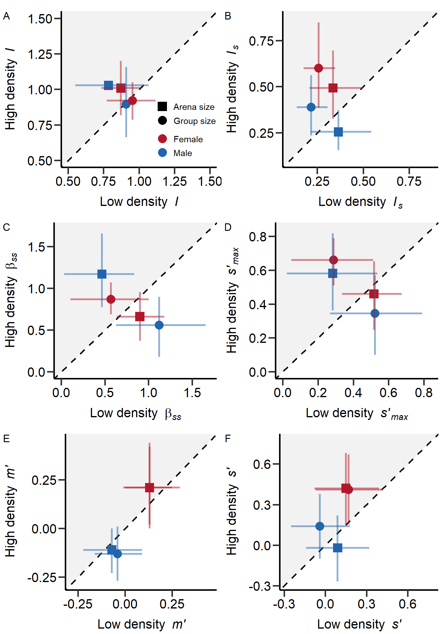
Figure 2: Selection metrics estimated for females (blue) and males (red) under density manipulated via group (point) or arena size (square). Opportunity for selection (I; A), opportunity for sexual selection (Is; B), Bateman gradient (βss; C), Jones index (s’max; D), mating differential on body mass (m’; E) and selection differential on body mass (s’; F) with mean and 95%CI estimated via bootstrapping. Dashed lines mark equal effect size for both densities. In grey area metrics were larger under high density treatments. The x-/y-distance of means from dashed line is equal to the effect size of the treatment.
Fig_2=plot_grid(Figure_2, ncol=1, rel_heights=c(0.1, 1)) # rel_heights values control title marginsAnalyses for sexual selection gradients
In the following we performed additional analyses on the sexual selection gradient.
GLM of sexual selection gradient for population size treatment
Males
GLM of sexual selection gradient for small population size treatment
bateman1=glm(rel_m_RS~rel_m_cMS,data=D_data_Small_pop) # Small population
summary(bateman1)
Call:
glm(formula = rel_m_RS ~ rel_m_cMS, data = D_data_Small_pop)

Deviance Residuals:
     Min        1Q    Median        3Q       Max
-1.26930  -0.56912  -0.00051   0.45026   2.19649

Coefficients:
            Estimate Std. Error t value Pr(>|t|)
(Intercept)  -0.1311     0.2832  -0.463    0.646
rel_m_cMS     1.1311     0.2567   4.407 6.64e-05 ***
---
Signif. codes:  0 '***' 0.001 '**' 0.01 '*' 0.05 '.' 0.1 ' ' 1

(Dispersion parameter for gaussian family taken to be 0.6588378)

    Null deviance: 41.784  on 45  degrees of freedom
Residual deviance: 28.989  on 44  degrees of freedom
  (54 Beobachtungen als fehlend gelöscht)
AIC: 115.3

Number of Fisher Scoring iterations: 2
GLM of sexual selection gradient for large population size treatment
bateman2=glm(rel_m_RS~rel_m_cMS,data=D_data_Large_pop) # Large population
summary(bateman2)
Call:
glm(formula = rel_m_RS ~ rel_m_cMS, data = D_data_Large_pop)

Deviance Residuals:
     Min        1Q    Median        3Q       Max
-1.74931  -0.71978  -0.06507   0.62329   2.29542

Coefficients:
            Estimate Std. Error t value Pr(>|t|)
(Intercept)   0.4380     0.2225   1.969  0.05394 .
rel_m_cMS     0.5620     0.1889   2.975  0.00432 **
---
Signif. codes:  0 '***' 0.001 '**' 0.01 '*' 0.05 '.' 0.1 ' ' 1

(Dispersion parameter for gaussian family taken to be 0.8012483)

    Null deviance: 51.961  on 57  degrees of freedom
Residual deviance: 44.870  on 56  degrees of freedom
  (45 Beobachtungen als fehlend gelöscht)
AIC: 155.71

Number of Fisher Scoring iterations: 2
Females
GLM of sexual selection gradient for small population size treatment
bateman3=glm(rel_f_RS~rel_f_cMS,data=D_data_Small_pop) # Small population
summary(bateman3)
Call:
glm(formula = rel_f_RS ~ rel_f_cMS, data = D_data_Small_pop)

Deviance Residuals:
    Min       1Q   Median       3Q      Max
-1.3281  -0.8177  -0.3007   0.7701   1.7421

Coefficients:
            Estimate Std. Error t value Pr(>|t|)
(Intercept)   0.4282     0.2862   1.496   0.1407
rel_f_cMS     0.5718     0.2553   2.239   0.0294 *
---
Signif. codes:  0 '***' 0.001 '**' 0.01 '*' 0.05 '.' 0.1 ' ' 1

(Dispersion parameter for gaussian family taken to be 0.902498)

    Null deviance: 51.456  on 53  degrees of freedom
Residual deviance: 46.930  on 52  degrees of freedom
  (46 Beobachtungen als fehlend gelöscht)
AIC: 151.67

Number of Fisher Scoring iterations: 2
GLM of sexual selection gradient for large population size treatment
bateman4=glm(rel_f_RS~rel_f_cMS,data=D_data_Large_pop) # Large population
summary(bateman4)
Call:
glm(formula = rel_f_RS ~ rel_f_cMS, data = D_data_Large_pop)

Deviance Residuals:
    Min       1Q   Median       3Q      Max
-1.1558  -0.6221  -0.1433   0.6154   1.2999

Coefficients:
            Estimate Std. Error t value Pr(>|t|)
(Intercept)   0.1433     0.1727   0.830    0.411
rel_f_cMS     0.8567     0.1366   6.273 1.46e-07 ***
---
Signif. codes:  0 '***' 0.001 '**' 0.01 '*' 0.05 '.' 0.1 ' ' 1

(Dispersion parameter for gaussian family taken to be 0.5026109)

    Null deviance: 41.393  on 44  degrees of freedom
Residual deviance: 21.612  on 43  degrees of freedom
  (58 Beobachtungen als fehlend gelöscht)
AIC: 100.7

Number of Fisher Scoring iterations: 2
GLM of sexual selection gradient for arena size treatment
Males
GLM of sexual selection gradient for small arena size treatment
bateman5=glm(rel_m_RS~rel_m_cMS,data=D_data_Small_arena) # Small arena
summary(bateman5)
Call:
glm(formula = rel_m_RS ~ rel_m_cMS, data = D_data_Small_arena)

Deviance Residuals:
     Min        1Q    Median        3Q       Max
-1.27592  -0.55853   0.02679   0.42022   2.17266

Coefficients:
            Estimate Std. Error t value Pr(>|t|)
(Intercept)  -0.1589     0.2688  -0.591    0.557
rel_m_cMS     1.1589     0.2400   4.828  1.5e-05 ***
---
Signif. codes:  0 '***' 0.001 '**' 0.01 '*' 0.05 '.' 0.1 ' ' 1

(Dispersion parameter for gaussian family taken to be 0.7161542)

    Null deviance: 50.353  on 48  degrees of freedom
Residual deviance: 33.659  on 47  degrees of freedom
  (48 Beobachtungen als fehlend gelöscht)
AIC: 126.65

Number of Fisher Scoring iterations: 2
GLM of sexual selection gradient for large arena size treatment
bateman6=glm(rel_m_RS~rel_m_cMS,data=D_data_Large_arena) # Large arena
summary(bateman6)
Call:
glm(formula = rel_m_RS ~ rel_m_cMS, data = D_data_Large_arena)

Deviance Residuals:
     Min        1Q    Median        3Q       Max
-1.63427  -0.57493  -0.05739   0.62351   2.33207

Coefficients:
            Estimate Std. Error t value Pr(>|t|)
(Intercept)   0.5243     0.2235   2.346   0.0228 *
rel_m_cMS     0.4757     0.1914   2.486   0.0161 *
---
Signif. codes:  0 '***' 0.001 '**' 0.01 '*' 0.05 '.' 0.1 ' ' 1

(Dispersion parameter for gaussian family taken to be 0.7332268)

    Null deviance: 43.393  on 54  degrees of freedom
Residual deviance: 38.861  on 53  degrees of freedom
  (51 Beobachtungen als fehlend gelöscht)
AIC: 142.98

Number of Fisher Scoring iterations: 2
Females
GLM of sexual selection gradient for small arena size treatment
bateman7=glm(rel_f_RS~rel_f_cMS,data=D_data_Small_arena) # Small arena
summary(bateman7)
Call:
glm(formula = rel_f_RS ~ rel_f_cMS, data = D_data_Small_arena)

Deviance Residuals:
    Min       1Q   Median       3Q      Max
-1.3172  -0.7534  -0.3397   0.7993   1.7657

Coefficients:
            Estimate Std. Error t value Pr(>|t|)
(Intercept)   0.3397     0.2285   1.487 0.143910
rel_f_cMS     0.6603     0.1870   3.531 0.000954 ***
---
Signif. codes:  0 '***' 0.001 '**' 0.01 '*' 0.05 '.' 0.1 ' ' 1

(Dispersion parameter for gaussian family taken to be 0.8267511)

    Null deviance: 48.338  on 47  degrees of freedom
Residual deviance: 38.031  on 46  degrees of freedom
  (49 Beobachtungen als fehlend gelöscht)
AIC: 131.04

Number of Fisher Scoring iterations: 2
GLM of sexual selection gradient for large arena size treatment
bateman8=glm(rel_f_RS~rel_f_cMS,data=D_data_Large_arena) # Large arena
summary(bateman8)
Call:
glm(formula = rel_f_RS ~ rel_f_cMS, data = D_data_Large_arena)

Deviance Residuals:
    Min       1Q   Median       3Q      Max
-1.5149  -0.5734  -0.1026   0.5860   1.6460

Coefficients:
            Estimate Std. Error t value Pr(>|t|)
(Intercept)   0.1026     0.2209   0.465    0.644
rel_f_cMS     0.8974     0.1911   4.696 2.17e-05 ***
---
Signif. codes:  0 '***' 0.001 '**' 0.01 '*' 0.05 '.' 0.1 ' ' 1

(Dispersion parameter for gaussian family taken to be 0.6264297)

    Null deviance: 44.511  on 50  degrees of freedom
Residual deviance: 30.695  on 49  degrees of freedom
  (55 Beobachtungen als fehlend gelöscht)
AIC: 124.84

Number of Fisher Scoring iterations: 2
Sexual selection gradient for all treatments combined (Global Bateman gradient)
Here we analysed the sexual selection gradient across all treatments for males and females.
D_data$rel_f_cMS=NA
D_data$rel_f_cMS=D_data$f_cMS/mean(D_data$f_cMS,na.rm=T)
D_data$rel_f_RS=NA
D_data$rel_f_RS=D_data$f_RS/mean(D_data$f_RS,na.rm=T)
D_data$rel_m_cMS=NA
D_data$rel_m_cMS=D_data$m_cMS/mean(D_data$m_cMS,na.rm=T)
D_data$rel_m_RS=NA
D_data$rel_m_RS=D_data$m_RS/mean(D_data$m_RS,na.rm=T)
Global sexual selection gradient of females:
bateman9=glm(rel_f_RS~rel_f_cMS+Body_mass_mg_focal,data=D_data)
summary(bateman9)
Call:
glm(formula = rel_f_RS ~ rel_f_cMS + Body_mass_mg_focal, data = D_data)

Deviance Residuals:
     Min        1Q    Median        3Q       Max
-1.58645  -0.65459  -0.07596   0.67662   1.84633

Coefficients:
                   Estimate Std. Error t value Pr(>|t|)
(Intercept)         -1.0206     0.6960  -1.467   0.1458
rel_f_cMS            0.7193     0.1320   5.451 3.88e-07 ***
Body_mass_mg_focal   0.5942     0.3259   1.823   0.0714 .
---
Signif. codes:  0 '***' 0.001 '**' 0.01 '*' 0.05 '.' 0.1 ' ' 1

(Dispersion parameter for gaussian family taken to be 0.6816762)

    Null deviance: 93.444  on 98  degrees of freedom
Residual deviance: 65.441  on 96  degrees of freedom
  (104 Beobachtungen als fehlend gelöscht)
AIC: 247.97

Number of Fisher Scoring iterations: 2
Global sexual selection gradient of males:
bateman10=glm(rel_m_RS~rel_m_cMS+Body_mass_mg_focal,data=D_data)
summary(bateman10)
Call:
glm(formula = rel_m_RS ~ rel_m_cMS + Body_mass_mg_focal, data = D_data)

Deviance Residuals:
    Min       1Q   Median       3Q      Max
-1.9470  -0.6320  -0.1481   0.4719   3.9252

Coefficients:
                   Estimate Std. Error t value Pr(>|t|)
(Intercept)         -0.6271     0.9108  -0.689    0.493
rel_m_cMS            0.7368     0.1603   4.597 1.25e-05 ***
Body_mass_mg_focal   0.4585     0.4467   1.027    0.307
---
Signif. codes:  0 '***' 0.001 '**' 0.01 '*' 0.05 '.' 0.1 ' ' 1

(Dispersion parameter for gaussian family taken to be 0.8262306)

    Null deviance: 100.985  on 103  degrees of freedom
Residual deviance:  83.449  on 101  degrees of freedom
  (99 Beobachtungen als fehlend gelöscht)
AIC: 280.24

Number of Fisher Scoring iterations: 2
Interaction between sexual selection gradient steepnes and sex
Next, we tested if the steepness of the global sexual selection gradient differed between the sexes.
data_combined=D_data
data_combined$rel_RS=NA
data_combined$rel_RS[data_combined$Sex=='M']=data_combined$rel_m_RS[data_combined$Sex=='M']
data_combined$rel_RS[data_combined$Sex=='F']=data_combined$rel_f_RS[data_combined$Sex=='F']
data_combined$rel_cMS=NA
data_combined$rel_cMS[data_combined$Sex=='M']=data_combined$rel_m_cMS[data_combined$Sex=='M']
data_combined$rel_cMS[data_combined$Sex=='F']=data_combined$rel_f_cMS[data_combined$Sex=='F']
Global sexual selection gradient with sex-interaction:
bateman11=glm(rel_RS~rel_cMS*Sex,data=data_combined)
summary(bateman11)
Call:
glm(formula = rel_RS ~ rel_cMS * Sex, data = data_combined)

Deviance Residuals:
    Min       1Q   Median       3Q      Max
-1.9987  -0.6759  -0.2175   0.6488   3.9222

Coefficients:
             Estimate Std. Error t value Pr(>|t|)
(Intercept)   0.21754    0.16090   1.352    0.178
rel_cMS       0.78246    0.13481   5.804 2.52e-08 ***
SexM          0.07145    0.23751   0.301    0.764
rel_cMS:SexM -0.07145    0.20334  -0.351    0.726
---
Signif. codes:  0 '***' 0.001 '**' 0.01 '*' 0.05 '.' 0.1 ' ' 1

(Dispersion parameter for gaussian family taken to be 0.7639526)

    Null deviance: 194.43  on 202  degrees of freedom
Residual deviance: 152.03  on 199  degrees of freedom
AIC: 527.39

Number of Fisher Scoring iterations: 2
Plot: Sexual selection gradient (Figure S6)
Finally, we plotted the sexual selection gradient for each sex and treatment.
p22<-ggplot(D_data_Small_pop, aes(x=rel_m_cMS, y=rel_m_RS)) +
  geom_point(alpha=0.4,shape=16, size = 3,color=colpal2[2]) +
  geom_smooth(method=lm, se=TRUE,alpha=0.3) +
  theme(plot.tag.position=c(0.1,0.98))+
  labs(tag = "A")+xlab('Rel. mating success')+ylab("Rel. reproductive success")+ggtitle('Small group')+ theme(plot.title = element_text(hjust = 0.5))+
  theme(axis.text=element_text(size=13),
        axis.title=element_text(size=14))+ theme(legend.position="none")+
  ylim(0,4.2)+xlim(0,3.2)+
  theme(panel.grid.major = element_blank(), panel.grid.minor = element_blank(),panel.background = element_blank(), axis.line = element_line(colour = "black"))
p22=p22+geom_point(aes(x=rel_f_cMS, y=rel_f_RS),color=colpal2[1],alpha=0.4,shape=16, size = 3)+
  geom_smooth(aes(x=rel_f_cMS, y=rel_f_RS),color=colpal2[1],method=lm, se=TRUE,alpha=0.3)

p23<-ggplot(D_data_Large_pop, aes(x=rel_m_cMS, y=rel_m_RS)) +
  geom_point(alpha=0.4,shape=16, size = 3,color=colpal2[2]) +
  geom_smooth(method=lm, se=TRUE,alpha=0.3) +
  theme(plot.tag.position=c(0.1,0.98))+
  labs(tag = "B")+xlab('Rel. mating success')+ylab("Rel. reproductive success")+ggtitle('Large group')+ theme(plot.title = element_text(hjust = 0.5))+
  theme(axis.text=element_text(size=13),
        axis.title=element_text(size=14))+ theme(legend.position="none")+
  ylim(0,4.2)+xlim(0,3.2)+
  theme(panel.grid.major = element_blank(), panel.grid.minor = element_blank(),panel.background = element_blank(), axis.line = element_line(colour = "black"))
p23=p23+geom_point(aes(x=rel_f_cMS, y=rel_f_RS),color=colpal2[1],alpha=0.4,shape=16, size = 3)+
  geom_smooth(aes(x=rel_f_cMS, y=rel_f_RS),color=colpal2[1],method=lm, se=TRUE,alpha=0.3)

p24<-ggplot(D_data_Large_arena, aes(x=rel_m_cMS, y=rel_m_RS)) +
  geom_point(alpha=0.4,shape=16, size = 3,color=colpal2[2]) +
  geom_smooth(method=lm, se=TRUE,alpha=0.3) +
  theme(plot.tag.position=c(0.1,0.98))+
  labs(tag = "C")+xlab('Rel. mating success')+ylab("Rel. reproductive success")+ggtitle('Large arena')+ theme(plot.title = element_text(hjust = 0.5))+
  theme(axis.text=element_text(size=13),
        axis.title=element_text(size=14))+ theme(legend.position="none")+
  ylim(0,4.2)+xlim(0,3.2)+
  theme(panel.grid.major = element_blank(), panel.grid.minor = element_blank(),panel.background = element_blank(), axis.line = element_line(colour = "black"))
p24=p24+geom_point(aes(x=rel_f_cMS, y=rel_f_RS),color=colpal2[1],alpha=0.4,shape=16, size = 3)+
  geom_smooth(aes(x=rel_f_cMS, y=rel_f_RS),color=colpal2[1],method=lm, se=TRUE,alpha=0.3)

p25<-ggplot(D_data_Small_arena, aes(x=rel_m_cMS, y=rel_m_RS)) +
  geom_point(alpha=0.4,shape=16, size = 3,color=colpal2[2]) +
  geom_smooth(method=lm, se=TRUE,alpha=0.3) +
  theme(plot.tag.position=c(0.1,0.98))+
  labs(tag = "D")+xlab('Rel. mating success')+ylab("Rel. reproductive success")+ggtitle('Small arena')+ theme(plot.title = element_text(hjust = 0.5))+
  theme(axis.text=element_text(size=13),
        axis.title=element_text(size=14))+
  ylim(0,4.2)+xlim(0,3.2)+
  theme(legend.position="none")+
  theme(panel.grid.major = element_blank(), panel.grid.minor = element_blank(),panel.background = element_blank(), axis.line = element_line(colour = "black"))
p25=p25+geom_point(aes(x=rel_f_cMS, y=rel_f_RS),color=colpal2[1],alpha=0.4,shape=16, size = 3)+
  geom_smooth(aes(x=rel_f_cMS, y=rel_f_RS),color=colpal2[1],method=lm, se=TRUE,alpha=0.3)

# Create legend
p26<-ggplot(D_data, aes(x=Total_N_MTP1, y=Total_N_Rd, color=Sex)) +
  geom_point(alpha=0.4,shape=16, size = 3, position=position_jitterdodge(jitter.height=0,jitter.width=0,dodge.width = 0)) +
  geom_smooth(method=lm, se=TRUE,alpha=0.3) +
  scale_color_manual(values=c(colpal2[1],colpal2[2]),name = "Sex", labels = c('Females','Males'))+
  xlab('Rel. mating success')+ylab("Rel. reproductive success")+
  guides(color=guide_legend(override.aes=list(fill=NA)))+
  theme(legend.key = element_rect(fill = "transparent"))

legend_Figure_S5 <- get_legend(p26)
Figure S5
Figure_S5<-grid.arrange(p22,p23,legend_Figure_S5,p24,p25,legend_Figure_S5, nrow = 2,ncol=3, widths=c(2.3, 2.3, 0.65))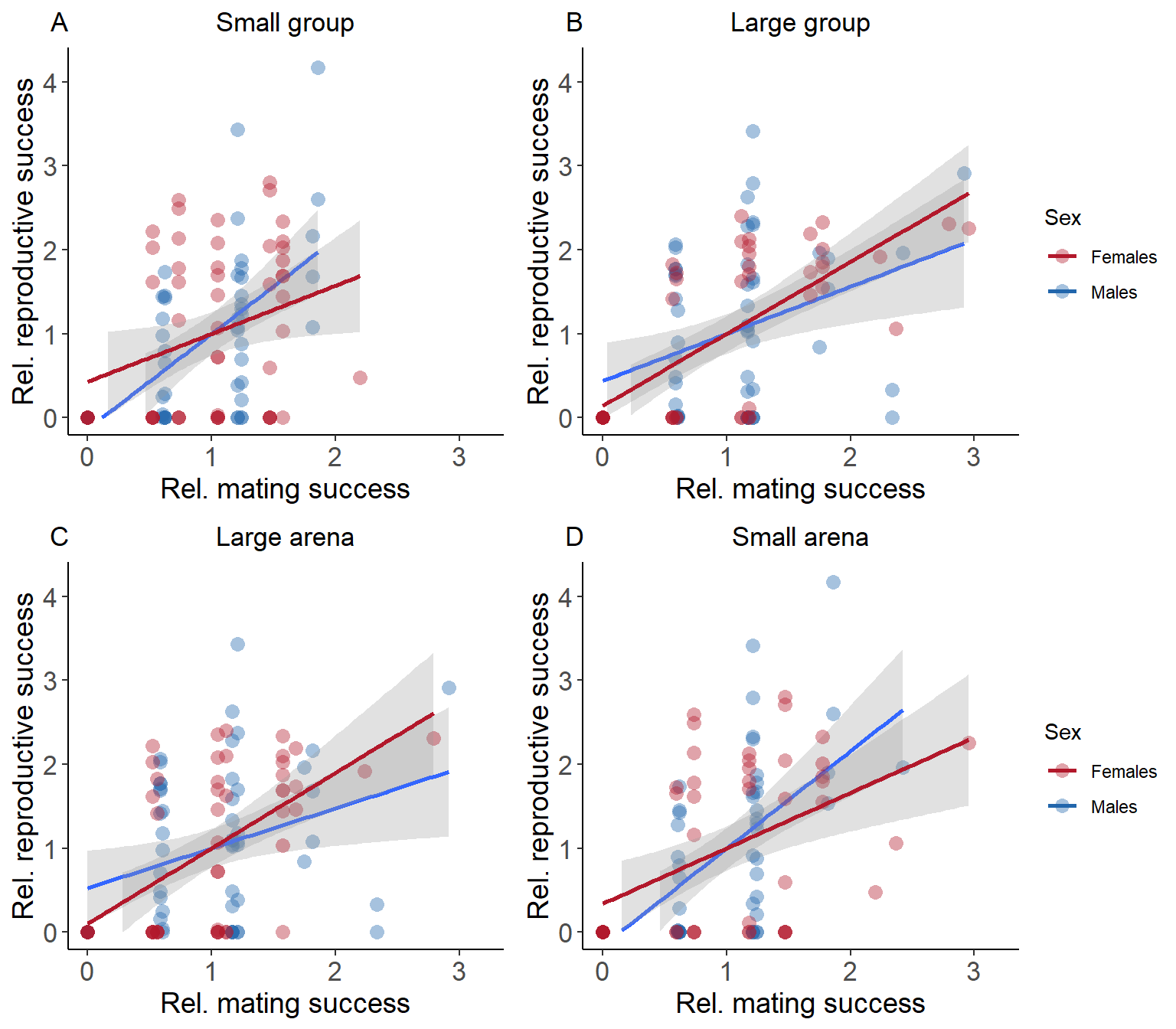
Figure S5: Scatterplot of Bateman gradients (βss; relativized mating success against relativized reproductive success) for males (blue) and females (red) for group size treatment (A + B) and arena size treatment (C+ D). Slopes of liner models estimating βss indicated by solid line with predicted 95% confidence intervals.
Fig_S5=plot_grid(Figure_S5, ncol=1, rel_heights=c(0.1, 1)) # rel_heights values control title marginsAnalyses for sexual selection gradients excluding individuals without mating success
Here we added an analysis of the sexual selection gradient excluding individuals that did not mate.
# Create data set excluding individuals without mating success
D_data_noZeroMS=D_data[D_data$MatingPartners_number!=0,]

## Merge data according to treatment
# Data according to denstiy
D_data_noZeroMS_0.26=D_data_noZeroMS[D_data_noZeroMS$Treatment=='D = 0.26',]
D_data_noZeroMS_0.52=D_data_noZeroMS[D_data_noZeroMS$Treatment=='D = 0.52',]
D_data_noZeroMS_0.67=D_data_noZeroMS[D_data_noZeroMS$Treatment=='D = 0.67',]
D_data_noZeroMS_1.33=D_data_noZeroMS[D_data_noZeroMS$Treatment=='D = 1.33',]

# Reduce treatments to arena and population size
# Arena size
D_data_noZeroMS_Large_arena=rbind(D_data_noZeroMS_0.26,D_data_noZeroMS_0.52)
D_data_noZeroMS_Small_arena=rbind(D_data_noZeroMS_0.67,D_data_noZeroMS_1.33)

# Population size
D_data_noZeroMS_Small_pop=rbind(D_data_noZeroMS_0.26,D_data_noZeroMS_0.67)
D_data_noZeroMS_Large_pop=rbind(D_data_noZeroMS_0.52,D_data_noZeroMS_1.33)
GLM of sexual selection gradient for population size treatment
Males
GLM of sexual selection gradient for population size treatment for small populations
bateman1=glm(rel_m_RS~rel_m_cMS,data=D_data_noZeroMS_Small_pop) # Small population
summary(bateman1)
Call:
glm(formula = rel_m_RS ~ rel_m_cMS, data = D_data_noZeroMS_Small_pop)

Deviance Residuals:
    Min       1Q   Median       3Q      Max
-1.4401  -0.6142  -0.2620   0.6026   3.2274

Coefficients:
            Estimate Std. Error t value Pr(>|t|)
(Intercept)  -0.2117     0.4450  -0.476  0.63674
rel_m_cMS     1.3739     0.3977   3.455  0.00129 **
---
Signif. codes:  0 '***' 0.001 '**' 0.01 '*' 0.05 '.' 0.1 ' ' 1

(Dispersion parameter for gaussian family taken to be 1.039294)

    Null deviance: 55.017  on 42  degrees of freedom
Residual deviance: 42.611  on 41  degrees of freedom
  (49 Beobachtungen als fehlend gelöscht)
AIC: 127.64

Number of Fisher Scoring iterations: 2
GLM of sexual selection gradient for population size treatment for large populations
bateman2=glm(rel_m_RS~rel_m_cMS,data=D_data_noZeroMS_Large_pop) # Large population
summary(bateman2)
Call:
glm(formula = rel_m_RS ~ rel_m_cMS, data = D_data_noZeroMS_Large_pop)

Deviance Residuals:
     Min        1Q    Median        3Q       Max
-1.32719  -0.78529  -0.01328   0.66413   1.84770

Coefficients:
            Estimate Std. Error t value Pr(>|t|)
(Intercept)   0.7035     0.2687   2.618   0.0117 *
rel_m_cMS     0.2594     0.2105   1.232   0.2237
---
Signif. codes:  0 '***' 0.001 '**' 0.01 '*' 0.05 '.' 0.1 ' ' 1

(Dispersion parameter for gaussian family taken to be 0.6673908)

    Null deviance: 33.716  on 50  degrees of freedom
Residual deviance: 32.702  on 49  degrees of freedom
  (34 Beobachtungen als fehlend gelöscht)
AIC: 128.07

Number of Fisher Scoring iterations: 2
Females
GLM of sexual selection gradient for population size treatment for small populations
bateman3=glm(rel_f_RS~rel_f_cMS,data=D_data_noZeroMS_Small_pop) # Small population
summary(bateman3)
Call:
glm(formula = rel_f_RS ~ rel_f_cMS, data = D_data_noZeroMS_Small_pop)

Deviance Residuals:
    Min       1Q   Median       3Q      Max
-1.4827  -0.8628   0.1097   0.8914   1.6975

Coefficients:
            Estimate Std. Error t value Pr(>|t|)
(Intercept)   0.5529     0.3855   1.434    0.158
rel_f_cMS     0.5291     0.3299   1.604    0.115

(Dispersion parameter for gaussian family taken to be 0.9707419)

    Null deviance: 48.122  on 48  degrees of freedom
Residual deviance: 45.625  on 47  degrees of freedom
  (43 Beobachtungen als fehlend gelöscht)
AIC: 141.56

Number of Fisher Scoring iterations: 2
GLM of sexual selection gradient for population size treatment for large populations
bateman4=glm(rel_f_RS~rel_f_cMS,data=D_data_noZeroMS_Large_pop) # Large population
summary(bateman4)
Call:
glm(formula = rel_f_RS ~ rel_f_cMS, data = D_data_noZeroMS_Large_pop)

Deviance Residuals:
     Min        1Q    Median        3Q       Max
-1.11690  -0.68093   0.01509   0.69916   1.10603

Coefficients:
            Estimate Std. Error t value Pr(>|t|)
(Intercept)   0.2450     0.3065   0.799  0.43005
rel_f_cMS     0.7442     0.2081   3.577  0.00113 **
---
Signif. codes:  0 '***' 0.001 '**' 0.01 '*' 0.05 '.' 0.1 ' ' 1

(Dispersion parameter for gaussian family taken to be 0.6033825)

    Null deviance: 27.029  on 33  degrees of freedom
Residual deviance: 19.308  on 32  degrees of freedom
  (51 Beobachtungen als fehlend gelöscht)
AIC: 83.25

Number of Fisher Scoring iterations: 2
GLM of sexual selection gradient for arena size treatment
Males
GLM of sexual selection gradient for arena size treatment for small arena
bateman5=glm(rel_m_RS~rel_m_cMS,data=D_data_noZeroMS_Small_arena) # Small arena
summary(bateman5)
Call:
glm(formula = rel_m_RS ~ rel_m_cMS, data = D_data_noZeroMS_Small_arena)

Deviance Residuals:
    Min       1Q   Median       3Q      Max
-1.3617  -0.5915  -0.1986   0.5709   3.3616

Coefficients:
            Estimate Std. Error t value Pr(>|t|)
(Intercept)  -0.1786     0.4209  -0.424  0.67338
rel_m_cMS     1.2812     0.3668   3.493  0.00112 **
---
Signif. codes:  0 '***' 0.001 '**' 0.01 '*' 0.05 '.' 0.1 ' ' 1

(Dispersion parameter for gaussian family taken to be 1.058743)

    Null deviance: 58.444  on 44  degrees of freedom
Residual deviance: 45.526  on 43  degrees of freedom
  (37 Beobachtungen als fehlend gelöscht)
AIC: 134.23

Number of Fisher Scoring iterations: 2
GLM of sexual selection gradient for arena size treatment for large arena
bateman6=glm(rel_m_RS~rel_m_cMS,data=D_data_noZeroMS_Large_arena) # Large arena
summary(bateman6)
Call:
glm(formula = rel_m_RS ~ rel_m_cMS, data = D_data_noZeroMS_Large_arena)

Deviance Residuals:
     Min        1Q    Median        3Q       Max
-1.26221  -0.69688  -0.03834   0.62374   2.14473

Coefficients:
            Estimate Std. Error t value Pr(>|t|)
(Intercept)   0.8186     0.2715   3.015  0.00413 **
rel_m_cMS     0.1845     0.2156   0.856  0.39655
---
Signif. codes:  0 '***' 0.001 '**' 0.01 '*' 0.05 '.' 0.1 ' ' 1

(Dispersion parameter for gaussian family taken to be 0.6466574)

    Null deviance: 30.866  on 48  degrees of freedom
Residual deviance: 30.393  on 47  degrees of freedom
  (46 Beobachtungen als fehlend gelöscht)
AIC: 121.65

Number of Fisher Scoring iterations: 2
Females
GLM of sexual selection gradient for arena size treatment for small arena
bateman7=glm(rel_f_RS~rel_f_cMS,data=D_data_noZeroMS_Small_arena) # Small arena
summary(bateman7)
Call:
glm(formula = rel_f_RS ~ rel_f_cMS, data = D_data_noZeroMS_Small_arena)

Deviance Residuals:
    Min       1Q   Median       3Q      Max
-1.1915  -0.8905   0.2676   0.8362   1.2729

Coefficients:
            Estimate Std. Error t value Pr(>|t|)
(Intercept)   0.5896     0.3552   1.660   0.1058
rel_f_cMS     0.5137     0.2788   1.843   0.0739 .
---
Signif. codes:  0 '***' 0.001 '**' 0.01 '*' 0.05 '.' 0.1 ' ' 1

(Dispersion parameter for gaussian family taken to be 0.8261488)

    Null deviance: 31.720  on 36  degrees of freedom
Residual deviance: 28.915  on 35  degrees of freedom
  (45 Beobachtungen als fehlend gelöscht)
AIC: 101.88

Number of Fisher Scoring iterations: 2
GLM of sexual selection gradient for arena size treatment for large arena
bateman8=glm(rel_f_RS~rel_f_cMS,data=D_data_noZeroMS_Large_arena) # Large arena
summary(bateman8)
Call:
glm(formula = rel_f_RS ~ rel_f_cMS, data = D_data_noZeroMS_Large_arena)

Deviance Residuals:
    Min       1Q   Median       3Q      Max
-1.5787  -0.6852  -0.1843   0.7460   1.8752

Coefficients:
            Estimate Std. Error t value Pr(>|t|)
(Intercept)   0.2384     0.3277   0.727  0.47079
rel_f_cMS     0.7627     0.2475   3.082  0.00355 **
---
Signif. codes:  0 '***' 0.001 '**' 0.01 '*' 0.05 '.' 0.1 ' ' 1

(Dispersion parameter for gaussian family taken to be 0.815707)

    Null deviance: 43.637  on 45  degrees of freedom
Residual deviance: 35.891  on 44  degrees of freedom
  (49 Beobachtungen als fehlend gelöscht)
AIC: 125.13

Number of Fisher Scoring iterations: 2
Sexual selection gradient for all treatments combined (Global Bateman gradient)
Here we analysed the sexual selection gradient across all treatments for males and females.
D_data_noZeroMS$rel_f_cMS=NA
D_data_noZeroMS$rel_f_cMS=D_data_noZeroMS$f_cMS/mean(D_data_noZeroMS$f_cMS,na.rm=T)
D_data_noZeroMS$rel_f_RS=NA
D_data_noZeroMS$rel_f_RS=D_data_noZeroMS$f_RS/mean(D_data_noZeroMS$f_RS,na.rm=T)
D_data_noZeroMS$rel_m_cMS=NA
D_data_noZeroMS$rel_m_cMS=D_data_noZeroMS$m_cMS/mean(D_data_noZeroMS$m_cMS,na.rm=T)
D_data_noZeroMS$rel_m_RS=NA
D_data_noZeroMS$rel_m_RS=D_data_noZeroMS$m_RS/mean(D_data_noZeroMS$m_RS,na.rm=T)
Global sexual selection gradient of females:
bateman9=glm(rel_f_RS~rel_f_cMS+Body_mass_mg_focal,data=D_data_noZeroMS)
summary(bateman9)
Call:
glm(formula = rel_f_RS ~ rel_f_cMS + Body_mass_mg_focal, data = D_data_noZeroMS)

Deviance Residuals:
     Min        1Q    Median        3Q       Max
-1.31733  -0.70473   0.04623   0.59495   1.49825

Coefficients:
                   Estimate Std. Error t value Pr(>|t|)
(Intercept)         -0.9513     0.7400  -1.285  0.20234
rel_f_cMS            0.6060     0.1851   3.274  0.00157 **
Body_mass_mg_focal   0.6063     0.3339   1.816  0.07308 .
---
Signif. codes:  0 '***' 0.001 '**' 0.01 '*' 0.05 '.' 0.1 ' ' 1

(Dispersion parameter for gaussian family taken to be 0.5711586)

    Null deviance: 54.962  on 82  degrees of freedom
Residual deviance: 45.693  on 80  degrees of freedom
  (94 Beobachtungen als fehlend gelöscht)
AIC: 194

Number of Fisher Scoring iterations: 2
Global sexual selection gradient of males:
bateman10=glm(rel_m_RS~rel_m_cMS+Body_mass_mg_focal,data=D_data_noZeroMS)
summary(bateman10)
Call:
glm(formula = rel_m_RS ~ rel_m_cMS + Body_mass_mg_focal, data = D_data_noZeroMS)

Deviance Residuals:
    Min       1Q   Median       3Q      Max
-1.6413  -0.6841  -0.0764   0.5487   3.6029

Coefficients:
                   Estimate Std. Error t value Pr(>|t|)
(Intercept)         -0.3193     0.9686  -0.330  0.74239
rel_m_cMS            0.6076     0.2101   2.892  0.00479 **
Body_mass_mg_focal   0.3657     0.4571   0.800  0.42578
---
Signif. codes:  0 '***' 0.001 '**' 0.01 '*' 0.05 '.' 0.1 ' ' 1

(Dispersion parameter for gaussian family taken to be 0.7392833)

    Null deviance: 73.460  on 93  degrees of freedom
Residual deviance: 67.275  on 91  degrees of freedom
  (83 Beobachtungen als fehlend gelöscht)
AIC: 243.32

Number of Fisher Scoring iterations: 2
Interaction between sexual selection gradient steepnes and sex
Next, we tested if the steepness of the global sexual selection gradient differed between the sexes.
data_combined=D_data_noZeroMS
data_combined$rel_RS=NA
data_combined$rel_RS[data_combined$Sex=='M']=data_combined$rel_m_RS[data_combined$Sex=='M']
data_combined$rel_RS[data_combined$Sex=='F']=data_combined$rel_f_RS[data_combined$Sex=='F']
data_combined$rel_cMS=NA
data_combined$rel_cMS[data_combined$Sex=='M']=data_combined$rel_m_cMS[data_combined$Sex=='M']
data_combined$rel_cMS[data_combined$Sex=='F']=data_combined$rel_f_cMS[data_combined$Sex=='F']
Global sexual selection gradient with sex-interaction:
bateman11=glm(rel_RS~rel_cMS*Sex,data=data_combined)
summary(bateman11)
Call:
glm(formula = rel_RS ~ rel_cMS * Sex, data = data_combined)

Deviance Residuals:
    Min       1Q   Median       3Q      Max
-1.6630  -0.6672   0.0023   0.6489   3.6092

Coefficients:
             Estimate Std. Error t value Pr(>|t|)
(Intercept)   0.34233    0.21697   1.578  0.11644
rel_cMS       0.65767    0.19759   3.328  0.00107 **
SexM          0.09265    0.30236   0.306  0.75966
rel_cMS:SexM -0.09265    0.27622  -0.335  0.73773
---
Signif. codes:  0 '***' 0.001 '**' 0.01 '*' 0.05 '.' 0.1 ' ' 1

(Dispersion parameter for gaussian family taken to be 0.6666166)

    Null deviance: 128.42  on 176  degrees of freedom
Residual deviance: 115.32  on 173  degrees of freedom
AIC: 436.48

Number of Fisher Scoring iterations: 2
Plot: Sexual selection gradient (Figure S7)
Finally, we plotted the sexual selection gradient for each sex and treatment.
p22<-ggplot(D_data_noZeroMS_Small_pop, aes(x=rel_m_cMS, y=rel_m_RS)) +
  geom_point(alpha=0.4,shape=16, size = 3,color=colpal2[2]) +
  geom_smooth(method=lm, se=TRUE,alpha=0.3) +
  theme(plot.tag.position=c(0.1,0.98))+
  labs(tag = "A")+xlab('Rel. mating success')+ylab("Rel. reproductive success")+ggtitle('Small group')+ theme(plot.title = element_text(hjust = 0.5))+
  theme(axis.text=element_text(size=13),
        axis.title=element_text(size=14))+ theme(legend.position="none")+
  ylim(0,4.2)+xlim(0,3.2)+
  theme(panel.grid.major = element_blank(), panel.grid.minor = element_blank(),panel.background = element_blank(), axis.line = element_line(colour = "black"))
p22=p22+geom_point(aes(x=rel_f_cMS, y=rel_f_RS),color=colpal2[1],alpha=0.4,shape=16, size = 3)+
  geom_smooth(aes(x=rel_f_cMS, y=rel_f_RS),color=colpal2[1],method=lm, se=TRUE,alpha=0.3)

p23<-ggplot(D_data_noZeroMS_Large_pop, aes(x=rel_m_cMS, y=rel_m_RS)) +
  geom_point(alpha=0.4,shape=16, size = 3,color=colpal2[2]) +
  geom_smooth(method=lm, se=TRUE,alpha=0.3) +
  theme(plot.tag.position=c(0.1,0.98))+
  labs(tag = "B")+xlab('Rel. mating success')+ylab("Rel. reproductive success")+ggtitle('Large group')+ theme(plot.title = element_text(hjust = 0.5))+
  theme(axis.text=element_text(size=13),
        axis.title=element_text(size=14))+ theme(legend.position="none")+
  ylim(0,4.2)+xlim(0,3.2)+
  theme(panel.grid.major = element_blank(), panel.grid.minor = element_blank(),panel.background = element_blank(), axis.line = element_line(colour = "black"))
p23=p23+geom_point(aes(x=rel_f_cMS, y=rel_f_RS),color=colpal2[1],alpha=0.4,shape=16, size = 3)+
  geom_smooth(aes(x=rel_f_cMS, y=rel_f_RS),color=colpal2[1],method=lm, se=TRUE,alpha=0.3)

p24<-ggplot(D_data_noZeroMS_Large_arena, aes(x=rel_m_cMS, y=rel_m_RS)) +
  geom_point(alpha=0.4,shape=16, size = 3,color=colpal2[2]) +
  geom_smooth(method=lm, se=TRUE,alpha=0.3) +
  theme(plot.tag.position=c(0.1,0.98))+
  labs(tag = "C")+xlab('Rel. mating success')+ylab("Rel. reproductive success")+ggtitle('Large arena')+ theme(plot.title = element_text(hjust = 0.5))+
  theme(axis.text=element_text(size=13),
        axis.title=element_text(size=14))+ theme(legend.position="none")+
  ylim(0,4.2)+xlim(0,3.2)+
  theme(panel.grid.major = element_blank(), panel.grid.minor = element_blank(),panel.background = element_blank(), axis.line = element_line(colour = "black"))
p24=p24+geom_point(aes(x=rel_f_cMS, y=rel_f_RS),color=colpal2[1],alpha=0.4,shape=16, size = 3)+
  geom_smooth(aes(x=rel_f_cMS, y=rel_f_RS),color=colpal2[1],method=lm, se=TRUE,alpha=0.3)

p25<-ggplot(D_data_noZeroMS_Small_arena, aes(x=rel_m_cMS, y=rel_m_RS)) +
  geom_point(alpha=0.4,shape=16, size = 3,color=colpal2[2]) +
  geom_smooth(method=lm, se=TRUE,alpha=0.3) +
  theme(plot.tag.position=c(0.1,0.98))+
  labs(tag = "D")+xlab('Rel. mating success')+ylab("Rel. reproductive success")+ggtitle('Small arena')+ theme(plot.title = element_text(hjust = 0.5))+
  theme(axis.text=element_text(size=13),
        axis.title=element_text(size=14))+
  ylim(0,4.2)+xlim(0,3.2)+
  theme(legend.position="none")+
  theme(panel.grid.major = element_blank(), panel.grid.minor = element_blank(),panel.background = element_blank(), axis.line = element_line(colour = "black"))
p25=p25+geom_point(aes(x=rel_f_cMS, y=rel_f_RS),color=colpal2[1],alpha=0.4,shape=16, size = 3)+
  geom_smooth(aes(x=rel_f_cMS, y=rel_f_RS),color=colpal2[1],method=lm, se=TRUE,alpha=0.3)

# Create legend
p26<-ggplot(D_data_noZeroMS, aes(x=Total_N_MTP1, y=Total_N_Rd, color=Sex)) +
  geom_point(alpha=0.4,shape=16, size = 3, position=position_jitterdodge(jitter.height=0,jitter.width=0,dodge.width = 0)) +
  geom_smooth(method=lm, se=TRUE,alpha=0.3) +
  scale_color_manual(values=c(colpal2[1],colpal2[2]),name = "Sex", labels = c('Females','Males'))+
  xlab('Rel. mating success')+ylab("Rel. reproductive success")+
  guides(color=guide_legend(override.aes=list(fill=NA)))+
  theme(legend.key = element_rect(fill = "transparent"))

legend_Figure_S6 <- get_legend(p26)
Figure S6
Figure_S6<-grid.arrange(p22,p23,legend_Figure_S6,p24,p25,legend_Figure_S6, nrow = 2,ncol=3, widths=c(2.3, 2.3, 0.65))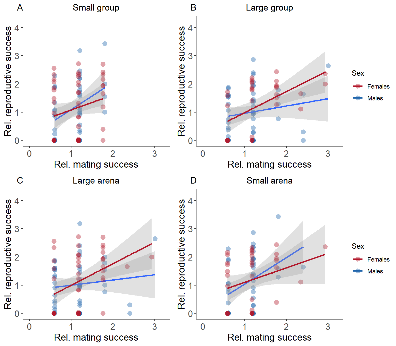
Figure S7: Scatterplot of Bateman gradients (βss; relativized mating success against relativized reproductive success) excluding individuals without mating success for males (blue) and females (red) for group size treatment (A + B) and arena size treatment (C+ D). Slopes of liner models estimating βss indicated by solid line with predicted 95% confidence intervals.
Fig_S6=plot_grid(Figure_S6, ncol=1, rel_heights=c(0.1, 1)) # rel_heights values control title marginsPermutation tests for treatment comparisons for (sexual) selection metrics
We used permutation tests to see if the (sexual) selection metrics differed between treatments.
## Permutation tests for treatment comparisons for (sexual) selection metrics ####
### Opportunity for sexual selection (I) ####
# Arena size
# Males
Treat_diff_Male_arena_I=c(I_Small_arena_Male_bootvar$t-c(I_Large_arena_Male_bootvar$t))

t_Treat_diff_Male_arena_I=mean(Treat_diff_Male_arena_I,na.rm=TRUE)
t_Treat_diff_Male_arena_I_lower=quantile(Treat_diff_Male_arena_I,.025,na.rm=TRUE)
t_Treat_diff_Male_arena_I_upper=quantile(Treat_diff_Male_arena_I,.975,na.rm=TRUE)

# Permutation test to calculate p value
comb_data=c(D_data_Large_arena$rel_m_RS,D_data_Small_arena$rel_m_RS)

diff.observed =  var(na.omit((D_data_Small_arena$rel_m_RS)))-var(na.omit((D_data_Large_arena$rel_m_RS)))
diff.observed

number_of_permutations = 100000
diff.random = NULL
for (i in 1 : number_of_permutations) {

  # Sample from the combined dataset
  a.random = sample (na.omit(comb_data), length(c(D_data_Large_arena$rel_m_RS)), TRUE)
  b.random = sample (na.omit(comb_data), length(c(D_data_Small_arena$rel_m_RS)), TRUE)

  # Null (permuated) difference
  diff.random[i] = var(na.omit(a.random)) - var(na.omit(b.random))
}

# P-value is the fraction of how many times the permuted difference is equal or more extreme than the observed difference

t_Treat_diff_Male_arena_I_p = sum(abs(diff.random) >= as.numeric(abs(diff.observed)))/   number_of_permutations

# Females
Treat_diff_Female_arena_I=c(I_Small_arena_Female_bootvar$t)-c(I_Large_arena_Female_bootvar$t)

t_Treat_diff_Female_arena_I=mean(Treat_diff_Female_arena_I,na.rm=TRUE)
t_Treat_diff_Female_arena_I_lower=quantile(Treat_diff_Female_arena_I,.025,na.rm=TRUE)
t_Treat_diff_Female_arena_I_upper=quantile(Treat_diff_Female_arena_I,.975,na.rm=TRUE)

# Permutation test to calculate p value
comb_data=c(D_data_Large_arena$rel_f_RS,D_data_Small_arena$rel_f_RS)

diff.observed =  var(na.omit((D_data_Small_arena$rel_f_RS)))-var(na.omit((D_data_Large_arena$rel_f_RS)))
diff.observed

number_of_permutations = 100000
diff.random = NULL
for (i in 1 : number_of_permutations) {

  # Sample from the combined dataset
  a.random = sample (na.omit(comb_data), length(c(D_data_Large_arena$rel_f_RS)), TRUE)
  b.random = sample (na.omit(comb_data), length(c(D_data_Small_arena$rel_f_RS)), TRUE)

  # Null (permuated) difference
  diff.random[i] = var(na.omit(a.random)) - var(na.omit(b.random))
}

# P-value is the fraction of how many times the permuted difference is equal or more extreme than the observed difference

t_Treat_diff_Female_arena_I_p = sum(abs(diff.random) >= as.numeric(abs(diff.observed)))/   number_of_permutations

# Population size
# Males
Treat_diff_Male_pop_I=c(I_Large_pop_Male_bootvar$t)-c(I_Small_pop_Male_bootvar$t)

t_Treat_diff_Male_pop_I=mean(Treat_diff_Male_pop_I,na.rm=TRUE)
t_Treat_diff_Male_pop_I_lower=quantile(Treat_diff_Male_pop_I,.025,na.rm=TRUE)
t_Treat_diff_Male_pop_I_upper=quantile(Treat_diff_Male_pop_I,.975,na.rm=TRUE)

# Permutation test to calculate p value
comb_data=c(D_data_Small_pop$rel_m_RS,D_data_Large_pop$rel_m_RS)

diff.observed =   var(na.omit((D_data_Large_pop$rel_m_RS)))-var(na.omit((D_data_Small_pop$rel_m_RS)))
diff.observed

number_of_permutations = 100000
diff.random = NULL
for (i in 1 : number_of_permutations) {

  # Sample from the combined dataset
  a.random = sample (na.omit(comb_data), length(c(D_data_Small_pop$rel_m_RS)), TRUE)
  b.random = sample (na.omit(comb_data), length(c(D_data_Large_pop$rel_m_RS)), TRUE)

  # Null (permuated) difference
  diff.random[i] = var(na.omit(a.random)) - var(na.omit(b.random))
}

# P-value is the fraction of how many times the permuted difference is equal or more extreme than the observed difference

t_Treat_diff_Male_pop_I_p = sum(abs(diff.random) >= as.numeric(abs(diff.observed)))/   number_of_permutations

# Females
Treat_diff_Female_pop_I=c(I_Large_pop_Female_bootvar$t)-c(I_Small_pop_Female_bootvar$t)

t_Treat_diff_Female_pop_I=mean(Treat_diff_Female_pop_I,na.rm=TRUE)
t_Treat_diff_Female_pop_I_lower=quantile(Treat_diff_Female_pop_I,.025,na.rm=TRUE)
t_Treat_diff_Female_pop_I_upper=quantile(Treat_diff_Female_pop_I,.975,na.rm=TRUE)

# Permutation test to calculate p value
comb_data=c(D_data_Small_pop$rel_f_RS,D_data_Large_pop$rel_f_RS)

diff.observed =   var(na.omit(c(D_data_Large_pop$rel_f_RS)))-var(na.omit(c(D_data_Small_pop$rel_f_RS)))
diff.observed

number_of_permutations = 100000
diff.random = NULL
for (i in 1 : number_of_permutations) {

  # Sample from the combined dataset
  a.random = sample (na.omit(comb_data), length(c(D_data_Small_pop$rel_f_RS)), TRUE)
  b.random = sample (na.omit(comb_data), length(c(D_data_Large_pop$rel_f_RS)), TRUE)

  # Null (permuated) difference
  diff.random[i] = var(na.omit(a.random)) - var(na.omit(b.random))
}

# P-value is the fraction of how many times the permuted difference is equal or more extreme than the observed difference

t_Treat_diff_Female_pop_I_p = sum(abs(diff.random) >= as.numeric(abs(diff.observed)))/   number_of_permutations

### Opportunity for sexual selection (Is) ####
# Arena size
# Males
Treat_diff_Male_arena_Is=c(Is_Small_arena_Male_bootvar$t)-c(Is_Large_arena_Male_bootvar$t)

t_Treat_diff_Male_arena_Is=mean(Treat_diff_Male_arena_Is,na.rm=TRUE)
t_Treat_diff_Male_arena_Is_lower=quantile(Treat_diff_Male_arena_Is,.025,na.rm=TRUE)
t_Treat_diff_Male_arena_Is_upper=quantile(Treat_diff_Male_arena_Is,.975,na.rm=TRUE)

# Permutation test to calculate p value
comb_data=c(D_data_Large_arena$rel_m_cMS,D_data_Small_arena$rel_m_cMS)

diff.observed =   var(na.omit(c(D_data_Small_arena$rel_m_cMS)))-var(na.omit(c(D_data_Large_arena$rel_m_cMS)))
diff.observed

number_of_permutations = 100000
diff.random = NULL
for (i in 1 : number_of_permutations) {

  # Sample from the combined dataset
  a.random = sample (na.omit(comb_data), length(c(D_data_Large_arena$rel_m_cMS)), TRUE)
  b.random = sample (na.omit(comb_data), length(c(D_data_Small_arena$rel_m_cMS)), TRUE)

  # Null (permuated) difference
  diff.random[i] = var(na.omit(a.random)) - var(na.omit(b.random))
}

# P-value is the fraction of how many times the permuted difference is equal or more extreme than the observed difference

t_Treat_diff_Male_arena_Is_p = sum(abs(diff.random) >= as.numeric(abs(diff.observed)))/   number_of_permutations

# Females
Treat_diff_Female_arena_Is=c(Is_Small_arena_Female_bootvar$t)-c(Is_Large_arena_Female_bootvar$t)

t_Treat_diff_Female_arena_Is=mean(Treat_diff_Female_arena_Is,na.rm=TRUE)
t_Treat_diff_Female_arena_Is_lower=quantile(Treat_diff_Female_arena_Is,.025,na.rm=TRUE)
t_Treat_diff_Female_arena_Is_upper=quantile(Treat_diff_Female_arena_Is,.975,na.rm=TRUE)

# Permutation test to calculate p value
comb_data=c(D_data_Large_arena$rel_f_cMS,D_data_Small_arena$rel_f_cMS)

diff.observed =  var(na.omit(c(D_data_Small_arena$rel_f_cMS)))-var(na.omit(c(D_data_Large_arena$rel_f_cMS)))
diff.observed

number_of_permutations = 100000
diff.random = NULL
for (i in 1 : number_of_permutations) {

  # Sample from the combined dataset
  a.random = sample (na.omit(comb_data), length(c(D_data_Large_arena$rel_f_cMS)), TRUE)
  b.random = sample (na.omit(comb_data), length(c(D_data_Small_arena$rel_f_cMS)), TRUE)

  # Null (permuated) difference
  diff.random[i] = var(na.omit(a.random)) - var(na.omit(b.random))
}

# P-value is the fraction of how many times the permuted difference is equal or more extreme than the observed difference

t_Treat_diff_Female_arena_Is_p = sum(abs(diff.random) >= as.numeric(abs(diff.observed)))/   number_of_permutations

# Population size
# Males
Treat_diff_Male_pop_Is=c(Is_Large_pop_Male_bootvar$t)-c(Is_Small_pop_Male_bootvar$t)

t_Treat_diff_Male_pop_Is=mean(Treat_diff_Male_pop_Is,na.rm=TRUE)
t_Treat_diff_Male_pop_Is_lower=quantile(Treat_diff_Male_pop_Is,.025,na.rm=TRUE)
t_Treat_diff_Male_pop_Is_upper=quantile(Treat_diff_Male_pop_Is,.975,na.rm=TRUE)

# Permutation test to calculate p value
comb_data=c(D_data_Small_pop$rel_m_cMS,D_data_Large_pop$rel_m_cMS)

diff.observed =  var(na.omit(D_data_Large_pop$rel_m_cMS))-var(na.omit(D_data_Small_pop$rel_m_cMS),na.rm = T)
diff.observed

number_of_permutations = 100000
diff.random = NULL
for (i in 1 : number_of_permutations) {

  # Sample from the combined dataset
  a.random = sample (na.omit(comb_data), length(D_data_Small_pop$rel_m_cMS), TRUE)
  b.random = sample (na.omit(comb_data), length(D_data_Large_pop$rel_m_cMS), TRUE)

  # Null (permuated) difference
  diff.random[i] = var(na.omit(a.random)) - var(na.omit(b.random))
}

# P-value is the fraction of how many times the permuted difference is equal or more extreme than the observed difference

t_Treat_diff_Male_pop_Is_p = sum(abs(diff.random) >= as.numeric(abs(diff.observed)))/   number_of_permutations

# Females
Treat_diff_Female_pop_Is=c(Is_Large_pop_Female_bootvar$t)-c(Is_Small_pop_Female_bootvar$t)

t_Treat_diff_Female_pop_Is=mean(Treat_diff_Female_pop_Is,na.rm=TRUE)
t_Treat_diff_Female_pop_Is_lower=quantile(Treat_diff_Female_pop_Is,.025,na.rm=TRUE)
t_Treat_diff_Female_pop_Is_upper=quantile(Treat_diff_Female_pop_Is,.975,na.rm=TRUE)

# Permutation test to calculate p value
comb_data=c(D_data_Small_pop$rel_f_cMS,D_data_Large_pop$rel_f_cMS)

diff.observed =  var(na.omit(D_data_Large_pop$rel_f_cMS))-var(na.omit(D_data_Small_pop$rel_f_cMS))
diff.observed

number_of_permutations = 100000
diff.random = NULL
for (i in 1 : number_of_permutations) {

  # Sample from the combined dataset
  a.random = sample (na.omit(comb_data), length(c(D_data_Small_pop$rel_f_cMS)), TRUE)
  b.random = sample (na.omit(comb_data), length(c(D_data_Large_pop$rel_f_cMS)), TRUE)

  # Null (permuated) difference
  diff.random[i] = var(na.omit(a.random)) - var(na.omit(b.random))
}

# P-value is the fraction of how many times the permuted difference is equal or more extreme than the observed difference

t_Treat_diff_Female_pop_Is_p = sum(abs(diff.random) >= as.numeric(abs(diff.observed)))/   number_of_permutations

### Sexual selection gradient ####
# Arena size
# Males
Treat_diff_Male_arena_B=c(B_Small_arena_Male_bootvar$t)-c(B_Large_arena_Male_bootvar$t)

t_Treat_diff_Male_arena_B=mean(Treat_diff_Male_arena_B,na.rm=TRUE)
t_Treat_diff_Male_arena_B_lower=quantile(Treat_diff_Male_arena_B,.025,na.rm=TRUE)
t_Treat_diff_Male_arena_B_upper=quantile(Treat_diff_Male_arena_B,.975,na.rm=TRUE)

# Permutation test to calculate p value
comb_data1=c(D_data_Large_arena$rel_m_RS, D_data_Small_arena$rel_m_RS)
comb_data2=c(D_data_Large_arena$rel_m_cMS,D_data_Small_arena$rel_m_cMS)

diff.observed =  lm(D_data_Small_arena$rel_m_RS ~D_data_Small_arena$rel_m_cMS)$coefficients[2]-lm(D_data_Large_arena$rel_m_RS ~D_data_Large_arena$rel_m_cMS)$coefficients[2]
diff.observed

number_of_permutations = 100000
diff.random = NULL
for (i in 1 : number_of_permutations) {

  # Sample from the combined dataset
  a.random = sample (na.omit(comb_data1), length(D_data_Large_arena$rel_m_RS), TRUE)
  b.random = sample (na.omit(comb_data1), length(D_data_Small_arena$rel_m_RS), TRUE)
  c.random = sample (na.omit(comb_data2), length(D_data_Large_arena$rel_m_cMS), TRUE)
  d.random = sample (na.omit(comb_data2), length(D_data_Small_arena$rel_m_cMS), TRUE)

  # Null (permuated) difference
  diff.random[i] = lm(b.random ~d.random)$coefficients[2]-lm(a.random ~c.random)$coefficients[2]
}

# P-value is the fraction of how many times the permuted difference is equal or more extreme than the observed difference

t_Treat_diff_Male_arena_B_p = sum(abs(diff.random) >= as.numeric(abs(diff.observed)))/   number_of_permutations

# Females
Treat_diff_Female_arena_B=c(B_Small_arena_Female_bootvar$t)-c(B_Large_arena_Female_bootvar$t)

t_Treat_diff_Female_arena_B=mean(Treat_diff_Female_arena_B,na.rm=TRUE)
t_Treat_diff_Female_arena_B_lower=quantile(Treat_diff_Female_arena_B,.025,na.rm=TRUE)
t_Treat_diff_Female_arena_B_upper=quantile(Treat_diff_Female_arena_B,.975,na.rm=TRUE)

# Permutation test to calculate p value
comb_data1=c(D_data_Large_arena$rel_f_RS, D_data_Small_arena$rel_f_RS)
comb_data2=c(D_data_Large_arena$rel_f_cMS,D_data_Small_arena$rel_f_cMS)

diff.observed =  lm(D_data_Small_arena$rel_f_RS ~D_data_Small_arena$rel_f_cMS)$coefficients[2]-lm(D_data_Large_arena$rel_f_RS ~D_data_Large_arena$rel_f_cMS)$coefficients[2]
diff.observed

number_of_permutations = 100000
diff.random = NULL
for (i in 1 : number_of_permutations) {

  # Sample from the combined dataset
  a.random = sample (na.omit(comb_data1), length(D_data_Large_arena$rel_f_RS), TRUE)
  b.random = sample (na.omit(comb_data1), length(D_data_Small_arena$rel_f_RS), TRUE)
  c.random = sample (na.omit(comb_data2), length(D_data_Large_arena$rel_f_cMS), TRUE)
  d.random = sample (na.omit(comb_data2), length(D_data_Small_arena$rel_f_cMS), TRUE)

  # Null (permuated) difference
  diff.random[i] = lm(b.random ~d.random)$coefficients[2]-lm(a.random ~c.random)$coefficients[2]
}

# P-value is the fraction of how many times the permuted difference is equal or more extreme than the observed difference

t_Treat_diff_Female_arena_B_p = sum(abs(diff.random) >= as.numeric(abs(diff.observed)))/   number_of_permutations

# Population size
# Males
Treat_diff_Male_pop_B=c(B_Large_pop_Male_bootvar$t)-c(B_Small_pop_Male_bootvar$t)

t_Treat_diff_Male_pop_B=mean(Treat_diff_Male_pop_B,na.rm=TRUE)
t_Treat_diff_Male_pop_B_lower=quantile(Treat_diff_Male_pop_B,.025,na.rm=TRUE)
t_Treat_diff_Male_pop_B_upper=quantile(Treat_diff_Male_pop_B,.975,na.rm=TRUE)

# Permutation test to calculate p value
comb_data1=c(D_data_Small_pop$rel_m_RS, D_data_Large_pop$rel_m_RS)
comb_data2=c(D_data_Small_pop$rel_m_cMS,D_data_Large_pop$rel_m_cMS)

diff.observed = lm(D_data_Large_pop$rel_m_RS ~D_data_Large_pop$rel_m_cMS)$coefficients[2]-lm(D_data_Small_pop$rel_m_RS ~D_data_Small_pop$rel_m_cMS)$coefficients[2]
diff.observed

number_of_permutations = 100000
diff.random = NULL
for (i in 1 : number_of_permutations) {

  # Sample from the combined dataset
  a.random = sample (na.omit(comb_data1), length(D_data_Small_pop$rel_m_RS), TRUE)
  b.random = sample (na.omit(comb_data1), length(D_data_Large_pop$rel_m_RS), TRUE)
  c.random = sample (na.omit(comb_data2), length(D_data_Small_pop$rel_m_cMS), TRUE)
  d.random = sample (na.omit(comb_data2), length(D_data_Large_pop$rel_m_cMS), TRUE)

  # Null (permuated) difference
  diff.random[i] =  lm(b.random ~d.random)$coefficients[2]-lm(a.random ~c.random)$coefficients[2]
}

# P-value is the fraction of how many times the permuted difference is equal or more extreme than the observed difference

t_Treat_diff_Male_pop_B_p = sum(abs(diff.random) >= as.numeric(abs(diff.observed)))/   number_of_permutations

# Females
Treat_diff_Female_pop_B=c(B_Large_pop_Female_bootvar$t)-c(B_Small_pop_Female_bootvar$t)

t_Treat_diff_Female_pop_B=mean(Treat_diff_Female_pop_B,na.rm=TRUE)
t_Treat_diff_Female_pop_B_lower=quantile(Treat_diff_Female_pop_B,.025,na.rm=TRUE)
t_Treat_diff_Female_pop_B_upper=quantile(Treat_diff_Female_pop_B,.975,na.rm=TRUE)

# Permutation test to calculate p value
comb_data1=c(D_data_Small_pop$rel_f_RS, D_data_Large_pop$rel_f_RS)
comb_data2=c(D_data_Small_pop$rel_f_cMS,D_data_Large_pop$rel_f_cMS)

diff.observed =  lm(D_data_Large_pop$rel_f_RS ~D_data_Large_pop$rel_f_cMS)$coefficients[2]-lm(D_data_Small_pop$rel_f_RS ~D_data_Small_pop$rel_f_cMS)$coefficients[2]
diff.observed

number_of_permutations = 100000
diff.random = NULL
for (i in 1 : number_of_permutations) {

  # Sample from the combined dataset
  a.random = sample (na.omit(comb_data1), length(D_data_Small_pop$rel_f_RS), TRUE)
  b.random = sample (na.omit(comb_data1), length(D_data_Large_pop$rel_f_RS), TRUE)
  c.random = sample (na.omit(comb_data2), length(D_data_Small_pop$rel_f_cMS), TRUE)
  d.random = sample (na.omit(comb_data2), length(D_data_Large_pop$rel_f_cMS), TRUE)

  # Null (permuated) difference
  diff.random[i] = lm(b.random ~d.random)$coefficients[2]-lm(a.random ~c.random)$coefficients[2]
}

# P-value is the fraction of how many times the permuted difference is equal or more extreme than the observed difference

t_Treat_diff_Female_pop_B_p = sum(abs(diff.random) >= as.numeric(abs(diff.observed)))/   number_of_permutations

### Jones index ####
# Arena size
# Males
Treat_diff_Male_arena_S=c(S_Small_arena_Male_bootvar$t)-c(S_Large_arena_Male_bootvar$t)

t_Treat_diff_Male_arena_S=mean(Treat_diff_Male_arena_S,na.rm=TRUE)
t_Treat_diff_Male_arena_S_lower=quantile(Treat_diff_Male_arena_S,.025,na.rm=TRUE)
t_Treat_diff_Male_arena_S_upper=quantile(Treat_diff_Male_arena_S,.975,na.rm=TRUE)

# Permutation test to calculate p value
comb_data1=c(D_data_Large_arena$rel_m_cMS, D_data_Small_arena$rel_m_cMS)
comb_data2=c(D_data_Large_arena$rel_m_RS, D_data_Small_arena$rel_m_RS)

diff.observed =  lm(D_data_Small_arena$rel_m_RS ~D_data_Small_arena$rel_m_cMS)$coefficients[2]*sqrt(var(D_data_Small_arena$rel_m_cMS, na.rm=TRUE))-lm(D_data_Large_arena$rel_m_RS ~D_data_Large_arena$rel_m_cMS)$coefficients[2]*sqrt(var(D_data_Large_arena$rel_m_cMS, na.rm=TRUE))
diff.observed

number_of_permutations = 100000
diff.random = NULL
for (i in 1 : number_of_permutations) {

  # Sample from the combined dataset
  a.random = sample (na.omit(comb_data1), length(D_data_Large_arena$rel_m_cMS), TRUE)
  b.random = sample (na.omit(comb_data1), length(D_data_Small_arena$rel_m_cMS), TRUE)
  c.random = sample (na.omit(comb_data2), length(D_data_Large_arena$rel_m_RS), TRUE)
  d.random = sample (na.omit(comb_data2), length(D_data_Small_arena$rel_m_RS), TRUE)

  # Null (permuated) difference
  diff.random[i] = lm(d.random ~b.random)$coefficients[2]*sqrt(var(b.random, na.rm=TRUE))-lm(c.random ~a.random)$coefficients[2]*sqrt(var(a.random, na.rm=TRUE))
}

# P-value is the fraction of how many times the permuted difference is equal or more extreme than the observed difference

t_Treat_diff_Male_arena_S_p = sum(abs(diff.random) >= as.numeric(abs(diff.observed)))/   number_of_permutations

# Females
Treat_diff_Female_arena_S=c(S_Small_arena_Female_bootvar$t)-c(S_Large_arena_Female_bootvar$t)

t_Treat_diff_Female_arena_S=mean(Treat_diff_Female_arena_S,na.rm=TRUE)
t_Treat_diff_Female_arena_S_lower=quantile(Treat_diff_Female_arena_S,.025,na.rm=TRUE)
t_Treat_diff_Female_arena_S_upper=quantile(Treat_diff_Female_arena_S,.975,na.rm=TRUE)

# Permutation test to calculate p value
comb_data1=c(D_data_Large_arena$rel_f_cMS, D_data_Small_arena$rel_f_cMS)
comb_data2=c(D_data_Large_arena$rel_f_RS, D_data_Small_arena$rel_f_RS)

diff.observed =  lm(D_data_Small_arena$rel_f_RS ~D_data_Small_arena$rel_f_cMS)$coefficients[2]*sqrt(var(D_data_Small_arena$rel_f_cMS, na.rm=TRUE))-lm(D_data_Large_arena$rel_f_RS ~D_data_Large_arena$rel_f_cMS)$coefficients[2]*sqrt(var(D_data_Large_arena$rel_f_cMS, na.rm=TRUE))
diff.observed

number_of_permutations = 100000
diff.random = NULL
for (i in 1 : number_of_permutations) {

  # Sample from the combined dataset
  a.random = sample (na.omit(comb_data1), length(D_data_Large_arena$rel_f_cMS), TRUE)
  b.random = sample (na.omit(comb_data1), length(D_data_Small_arena$rel_f_cMS), TRUE)
  c.random = sample (na.omit(comb_data2), length(D_data_Large_arena$rel_f_RS), TRUE)
  d.random = sample (na.omit(comb_data2), length(D_data_Small_arena$rel_f_RS), TRUE)

  # Null (permuated) difference
  diff.random[i] = lm(d.random ~b.random)$coefficients[2]*sqrt(var(b.random, na.rm=TRUE))-lm(c.random ~a.random)$coefficients[2]*sqrt(var(a.random, na.rm=TRUE))
}

# P-value is the fraction of how many times the permuted difference is equal or more extreme than the observed difference

t_Treat_diff_Female_arena_S_p = sum(abs(diff.random) >= as.numeric(abs(diff.observed)))/   number_of_permutations

# Population size
# Males
Treat_diff_Male_pop_S=c(S_Large_pop_Male_bootvar$t)-c(S_Small_pop_Male_bootvar$t)

t_Treat_diff_Male_pop_S=mean(Treat_diff_Male_pop_S,na.rm=TRUE)
t_Treat_diff_Male_pop_S_lower=quantile(Treat_diff_Male_pop_S,.025,na.rm=TRUE)
t_Treat_diff_Male_pop_S_upper=quantile(Treat_diff_Male_pop_S,.975,na.rm=TRUE)

# Permutation test to calculate p value
comb_data1=c(D_data_Small_pop$rel_m_cMS, D_data_Large_pop$rel_m_cMS)
comb_data2=c(D_data_Small_pop$rel_m_RS, D_data_Large_pop$rel_m_RS)

diff.observed = lm(D_data_Large_pop$rel_m_RS ~D_data_Large_pop$rel_m_cMS)$coefficients[2]*sqrt(var(D_data_Large_pop$rel_m_cMS, na.rm=TRUE))-lm(D_data_Small_pop$rel_m_RS ~D_data_Small_pop$rel_m_cMS)$coefficients[2]*sqrt(var(D_data_Small_pop$rel_m_cMS, na.rm=TRUE))
diff.observed

number_of_permutations = 100000
diff.random = NULL
for (i in 1 : number_of_permutations) {

  # Sample from the combined dataset
  a.random = sample (na.omit(comb_data1), length(D_data_Small_pop$rel_m_cMS), TRUE)
  b.random = sample (na.omit(comb_data1), length(D_data_Large_pop$rel_m_cMS), TRUE)
  c.random = sample (na.omit(comb_data2), length(D_data_Small_pop$rel_m_RS), TRUE)
  d.random = sample (na.omit(comb_data2), length(D_data_Large_pop$rel_m_RS), TRUE)

  # Null (permuated) difference
  diff.random[i] =  lm(d.random ~b.random)$coefficients[2]*sqrt(var(b.random, na.rm=TRUE))-lm(c.random ~a.random)$coefficients[2]*sqrt(var(a.random, na.rm=TRUE))
}

# P-value is the fraction of how many times the permuted difference is equal or more extreme than the observed difference

t_Treat_diff_Male_pop_S_p = sum(abs(diff.random) >= as.numeric(abs(diff.observed)))/   number_of_permutations

# Females
Treat_diff_Female_pop_S=c(S_Large_pop_Female_bootvar$t)-c(S_Small_pop_Female_bootvar$t)

t_Treat_diff_Female_pop_S=mean(Treat_diff_Female_pop_S,na.rm=TRUE)
t_Treat_diff_Female_pop_S_lower=quantile(Treat_diff_Female_pop_S,.025,na.rm=TRUE)
t_Treat_diff_Female_pop_S_upper=quantile(Treat_diff_Female_pop_S,.975,na.rm=TRUE)

# Permutation test to calculate p value
comb_data1=c(D_data_Small_pop$rel_f_cMS, D_data_Large_pop$rel_f_cMS)
comb_data2=c(D_data_Small_pop$rel_f_RS, D_data_Large_pop$rel_f_RS)

diff.observed = lm(D_data_Large_pop$rel_f_RS ~D_data_Large_pop$rel_f_cMS)$coefficients[2]*sqrt(var(D_data_Large_pop$rel_f_cMS, na.rm=TRUE))-lm(D_data_Small_pop$rel_f_RS ~D_data_Small_pop$rel_f_cMS)$coefficients[2]*sqrt(var(D_data_Small_pop$rel_f_cMS, na.rm=TRUE))
diff.observed

number_of_permutations = 100000
diff.random = NULL
for (i in 1 : number_of_permutations) {

  # Sample from the combined dataset
  a.random = sample (na.omit(comb_data1), length(D_data_Small_pop$rel_f_cMS), TRUE)
  b.random = sample (na.omit(comb_data1), length(D_data_Large_pop$rel_f_cMS), TRUE)
  c.random = sample (na.omit(comb_data2), length(D_data_Small_pop$rel_f_RS), TRUE)
  d.random = sample (na.omit(comb_data2), length(D_data_Large_pop$rel_f_RS), TRUE)

  # Null (permuated) difference
  diff.random[i] =  lm(d.random ~b.random)$coefficients[2]*sqrt(var(b.random, na.rm=TRUE))-lm(c.random ~a.random)$coefficients[2]*sqrt(var(a.random, na.rm=TRUE))
}

# P-value is the fraction of how many times the permuted difference is equal or more extreme than the observed difference

t_Treat_diff_Female_pop_S_p = sum(abs(diff.random) >= as.numeric(abs(diff.observed)))/   number_of_permutations

### Extract data and write results table ####
CompTreat_Table_Male_arena_I <- as.data.frame(cbind("Male", "Arena size", "Opportunity for selection", t_Treat_diff_Male_arena_I, t_Treat_diff_Male_arena_I_lower, t_Treat_diff_Male_arena_I_upper, t_Treat_diff_Male_arena_I_p))
names(CompTreat_Table_Male_arena_I)=c('V1','V2','V3','V4','V5','V6','V7')
CompTreat_Table_Male_pop_I <- as.data.frame(cbind("Male", "Population size", "Opportunity for selection", t_Treat_diff_Male_pop_I, t_Treat_diff_Male_pop_I_lower, t_Treat_diff_Male_pop_I_upper, t_Treat_diff_Male_pop_I_p))
names(CompTreat_Table_Male_pop_I)=c('V1','V2','V3','V4','V5','V6','V7')
CompTreat_Table_Male_arena_Is <- as.data.frame(cbind("Male", "Arena size", "Opportunity for sexual selection", t_Treat_diff_Male_arena_Is, t_Treat_diff_Male_arena_Is_lower, t_Treat_diff_Male_arena_Is_upper, t_Treat_diff_Male_arena_Is_p))
names(CompTreat_Table_Male_arena_Is)=c('V1','V2','V3','V4','V5','V6','V7')
CompTreat_Table_Male_pop_Is <- as.data.frame(cbind("Male", "Population size", "Opportunity for sexual selection", t_Treat_diff_Male_pop_Is, t_Treat_diff_Male_pop_Is_lower, t_Treat_diff_Male_pop_Is_upper, t_Treat_diff_Male_pop_Is_p))
names(CompTreat_Table_Male_pop_Is)=c('V1','V2','V3','V4','V5','V6','V7')
CompTreat_Table_Male_arena_B <- as.data.frame(cbind("Male", "Arena size", "Bateman gradient", t_Treat_diff_Male_arena_B, t_Treat_diff_Male_arena_B_lower, t_Treat_diff_Male_arena_B_upper, t_Treat_diff_Male_arena_B_p))
names(CompTreat_Table_Male_arena_B)=c('V1','V2','V3','V4','V5','V6','V7')
CompTreat_Table_Male_pop_B <- as.data.frame(cbind("Male", "Population size", "Bateman gradient", t_Treat_diff_Male_pop_B, t_Treat_diff_Male_pop_B_lower, t_Treat_diff_Male_pop_B_upper, t_Treat_diff_Male_pop_B_p))
names(CompTreat_Table_Male_pop_B)=c('V1','V2','V3','V4','V5','V6','V7')
CompTreat_Table_Male_arena_S <- as.data.frame(cbind("Male", "Arena size", "Jones index", t_Treat_diff_Male_arena_S, t_Treat_diff_Male_arena_S_lower, t_Treat_diff_Male_arena_S_upper, t_Treat_diff_Male_arena_S_p))
names(CompTreat_Table_Male_arena_S)=c('V1','V2','V3','V4','V5','V6','V7')
CompTreat_Table_Male_pop_S <- as.data.frame(cbind("Male", "Population size", "Jones index", t_Treat_diff_Male_pop_S, t_Treat_diff_Male_pop_S_lower, t_Treat_diff_Male_pop_S_upper, t_Treat_diff_Male_pop_S_p))
names(CompTreat_Table_Male_pop_S)=c('V1','V2','V3','V4','V5','V6','V7')
CompTreat_Table_Female_arena_I <- as.data.frame(cbind("Female", "Arena size", "Opportunity for selection", t_Treat_diff_Female_arena_I, t_Treat_diff_Female_arena_I_lower, t_Treat_diff_Female_arena_I_upper, t_Treat_diff_Female_arena_I_p))
names(CompTreat_Table_Female_arena_I)=c('V1','V2','V3','V4','V5','V6','V7')
CompTreat_Table_Female_pop_I <- as.data.frame(cbind("Female", "Population size", "Opportunity for selection", t_Treat_diff_Female_pop_I, t_Treat_diff_Female_pop_I_lower, t_Treat_diff_Female_pop_I_upper, t_Treat_diff_Female_pop_I_p))
names(CompTreat_Table_Female_pop_I)=c('V1','V2','V3','V4','V5','V6','V7')
CompTreat_Table_Female_arena_Is <- as.data.frame(cbind("Female", "Arena size", "Opportunity for sexual selection", t_Treat_diff_Female_arena_Is, t_Treat_diff_Female_arena_Is_lower, t_Treat_diff_Female_arena_Is_upper, t_Treat_diff_Female_arena_Is_p))
names(CompTreat_Table_Female_arena_Is)=c('V1','V2','V3','V4','V5','V6','V7')
CompTreat_Table_Female_pop_Is <- as.data.frame(cbind("Female", "Population size", "Opportunity for sexual selection", t_Treat_diff_Female_pop_Is, t_Treat_diff_Female_pop_Is_lower, t_Treat_diff_Female_pop_Is_upper, t_Treat_diff_Female_pop_Is_p))
names(CompTreat_Table_Female_pop_Is)=c('V1','V2','V3','V4','V5','V6','V7')
CompTreat_Table_Female_arena_B <- as.data.frame(cbind("Female", "Arena size", "Bateman gradient", t_Treat_diff_Female_arena_B, t_Treat_diff_Female_arena_B_lower, t_Treat_diff_Female_arena_B_upper, t_Treat_diff_Female_arena_B_p))
names(CompTreat_Table_Female_arena_B)=c('V1','V2','V3','V4','V5','V6','V7')
CompTreat_Table_Female_pop_B <- as.data.frame(cbind("Female", "Population size", "Bateman gradient", t_Treat_diff_Female_pop_B, t_Treat_diff_Female_pop_B_lower, t_Treat_diff_Female_pop_B_upper, t_Treat_diff_Female_pop_B_p))
names(CompTreat_Table_Female_pop_B)=c('V1','V2','V3','V4','V5','V6','V7')
CompTreat_Table_Female_arena_S <- as.data.frame(cbind("Female", "Arena size", "Jones index", t_Treat_diff_Female_arena_S, t_Treat_diff_Female_arena_S_lower, t_Treat_diff_Female_arena_S_upper, t_Treat_diff_Female_arena_S_p))
names(CompTreat_Table_Female_arena_S)=c('V1','V2','V3','V4','V5','V6','V7')
CompTreat_Table_Female_pop_S <- as.data.frame(cbind("Female", "Population size", "Jones index", t_Treat_diff_Female_pop_S, t_Treat_diff_Female_pop_S_lower, t_Treat_diff_Female_pop_S_upper, t_Treat_diff_Female_pop_S_p))
names(CompTreat_Table_Female_pop_S)=c('V1','V2','V3','V4','V5','V6','V7')

Table_BatemanMetrics_TreatComp <- as.data.frame(as.matrix(rbind(CompTreat_Table_Male_arena_I,CompTreat_Table_Male_arena_Is,
                                                                CompTreat_Table_Male_arena_B,CompTreat_Table_Male_arena_S,
                                                                CompTreat_Table_Male_pop_I,CompTreat_Table_Male_pop_Is,
                                                                CompTreat_Table_Male_pop_B,CompTreat_Table_Male_pop_S,
                                                                CompTreat_Table_Female_arena_I,CompTreat_Table_Female_arena_Is,
                                                                CompTreat_Table_Female_arena_B,CompTreat_Table_Female_arena_S,
                                                                CompTreat_Table_Female_pop_I,CompTreat_Table_Female_pop_Is,
                                                                CompTreat_Table_Female_pop_B,CompTreat_Table_Female_pop_S
)))

Table_BatemanMetrics_TreatComp[,4]=as.numeric(Table_BatemanMetrics_TreatComp[,4])
Table_BatemanMetrics_TreatComp[,5]=as.numeric(Table_BatemanMetrics_TreatComp[,5])
Table_BatemanMetrics_TreatComp[,6]=as.numeric(Table_BatemanMetrics_TreatComp[,6])
Table_BatemanMetrics_TreatComp[,7]=as.numeric(Table_BatemanMetrics_TreatComp[,7])

colnames(Table_BatemanMetrics_TreatComp)[1] <- "Sex"
colnames(Table_BatemanMetrics_TreatComp)[2] <- "Treatment"
colnames(Table_BatemanMetrics_TreatComp)[3] <- "Selection_metric"
colnames(Table_BatemanMetrics_TreatComp)[4] <- "Variance"
colnames(Table_BatemanMetrics_TreatComp)[5] <- "l95_CI"
colnames(Table_BatemanMetrics_TreatComp)[6] <- "u95_CI"
colnames(Table_BatemanMetrics_TreatComp)[7] <- "p-value"
Table_BatemanMetrics_TreatComp[,4]=round(as.numeric(Table_BatemanMetrics_TreatComp[,4]),digits=2)
Table_BatemanMetrics_TreatComp[,5]=round(as.numeric(Table_BatemanMetrics_TreatComp[,5]),digits=2)
Table_BatemanMetrics_TreatComp[,6]=round(as.numeric(Table_BatemanMetrics_TreatComp[,6]),digits=2)
Table_BatemanMetrics_TreatComp[,7]=round(as.numeric(Table_BatemanMetrics_TreatComp[,7]),digits=3)
rownames(Table_BatemanMetrics_TreatComp) <- c()
Table A1: Treatment comparisons for sexual selection metrics including 95% confidence intervals. Negative effect sizes indicate larger values at lower density and positive effect sizes larger values at higher density.
kable(Table_BatemanMetrics_TreatComp)| Sex | Treatment | Selection_metric | Variance | l95_CI | u95_CI | p-value |
|---|---|---|---|---|---|---|
| Male | Arena size | Opportunity for selection | 0.24 | -0.25 | 0.81 | 0.184 |
| Male | Arena size | Opportunity for sexual selection | -0.11 | -0.32 | 0.08 | 0.129 |
| Male | Arena size | Bateman gradient | 0.70 | 0.14 | 1.33 | 0.005 |
| Male | Arena size | Jones index | 0.30 | -0.04 | 0.65 | 0.026 |
| Male | Population size | Opportunity for selection | -0.02 | -0.59 | 0.48 | 0.927 |
| Male | Population size | Opportunity for sexual selection | 0.17 | -0.01 | 0.36 | 0.021 |
| Male | Population size | Bateman gradient | -0.56 | -1.22 | 0.06 | 0.020 |
| Male | Population size | Jones index | -0.18 | -0.54 | 0.17 | 0.179 |
| Female | Arena size | Opportunity for selection | 0.14 | -0.10 | 0.37 | 0.088 |
| Female | Arena size | Opportunity for sexual selection | 0.16 | -0.08 | 0.40 | 0.060 |
| Female | Arena size | Bateman gradient | -0.24 | -0.63 | 0.15 | 0.271 |
| Female | Arena size | Jones index | -0.06 | -0.32 | 0.21 | 0.677 |
| Female | Population size | Opportunity for selection | -0.03 | -0.26 | 0.19 | 0.712 |
| Female | Population size | Opportunity for sexual selection | 0.34 | 0.11 | 0.60 | 0.000 |
| Female | Population size | Bateman gradient | 0.30 | -0.18 | 0.80 | 0.185 |
| Female | Population size | Jones index | 0.37 | 0.11 | 0.65 | 0.005 |
Permutation test for treatment effect on mating differential of body mass
We used permutation tests to see if the mating differential of body mass differed between treatments.
## Permutation test for treatment effect on mating differential of body mass ####
# Group size
# Males
Treat_diff_male_pop=c(boot_BW_males_group_size_large$t)-c(boot_BW_males_group_size_small$t)

t_Treat_diff_male_pop=mean(Treat_diff_male_pop,na.rm=TRUE)
t_Treat_diff_male_pop_lower=quantile(Treat_diff_male_pop,.025,na.rm=TRUE)
t_Treat_diff_male_pop_upper=quantile(Treat_diff_male_pop,.975,na.rm=TRUE)

# Permutation test to calculate p value
comb_data_RS=c(D_data_m[D_data_m$Gr_size=='LG',]$m_cMS/mean(D_data_m[D_data_m$Gr_size=='LG',]$m_cMS),
               D_data_m[D_data_m$Gr_size=='SG',]$m_cMS/mean(D_data_m[D_data_m$Gr_size=='SG',]$m_cMS))
comb_data_BM=c(D_data_m[D_data_m$Gr_size=='LG',]$stder_BM_focal,
               D_data_m[D_data_m$Gr_size=='SG',]$stder_BM_focal)

diff.observed_male_pop = cov(D_data_m[D_data_m$Gr_size=='LG',]$stder_BM_focal,D_data_m[D_data_m$Gr_size=='LG',]$m_cMS/mean(D_data_m[D_data_m$Gr_size=='LG',]$m_cMS),use="complete.obs",method = "pearson") - cov(D_data_m[D_data_m$Gr_size=='SG',]$stder_BM_focal,D_data_m[D_data_m$Gr_size=='SG',]$m_cMS/mean(D_data_m[D_data_m$Gr_size=='SG',]$m_cMS),use="complete.obs",method = "pearson")

number_of_permutations = 100000
diff.random_male_pop = NULL
for (i in 1 : number_of_permutations) {

  # Sample from the combined dataset
  a.random = sample (na.omit(comb_data_RS), length(c(D_data_m[D_data_m$Gr_size=='LG',]$m_cMS/mean(D_data_m[D_data_m$Gr_size=='LG',]$m_cMS))), TRUE)
  b.random = sample (na.omit(comb_data_BM), length(c(D_data_m[D_data_m$Gr_size=='LG',]$m_cMS/mean(D_data_m[D_data_m$Gr_size=='LG',]$m_cMS))), TRUE)
  c.random = sample (na.omit(comb_data_RS), length(c(D_data_m[D_data_m$Gr_size=='SG',]$m_cMS/mean(D_data_m[D_data_m$Gr_size=='SG',]$m_cMS))), TRUE)
  d.random = sample (na.omit(comb_data_BM), length(c(D_data_m[D_data_m$Gr_size=='SG',]$m_cMS/mean(D_data_m[D_data_m$Gr_size=='SG',]$m_cMS))), TRUE)

  # Null (permuated) difference
  diff.random_male_pop[i] = cov(b.random,a.random,use="complete.obs",method = "pearson") - cov(d.random,c.random,use="complete.obs",method = "pearson")
}

# P-value is the fraction of how many times the permuted difference is equal or more extreme than the observed difference

p_Treat_diff_male_pop = sum(abs(diff.random_male_pop) >= as.numeric(abs(diff.observed_male_pop)))/   number_of_permutations

# Females
Treat_diff_female_pop=c(boot_BW_females_group_size_large$t)-c(boot_BW_females_group_size_small$t)

t_Treat_diff_female_pop=mean(Treat_diff_female_pop,na.rm=TRUE)
t_Treat_diff_female_pop_lower=quantile(Treat_diff_female_pop,.025,na.rm=TRUE)
t_Treat_diff_female_pop_upper=quantile(Treat_diff_female_pop,.975,na.rm=TRUE)

# Permutation test to calculate p value
comb_data_RS=c(D_data_f[D_data_f$Gr_size=='LG',]$f_cMS/mean(D_data_f[D_data_f$Gr_size=='LG',]$f_cMS),
               D_data_f[D_data_f$Gr_size=='SG',]$f_cMS/mean(D_data_f[D_data_f$Gr_size=='SG',]$f_cMS))
comb_data_BM=c(D_data_f[D_data_f$Gr_size=='LG',]$stder_BM_focal,
               D_data_f[D_data_f$Gr_size=='SG',]$stder_BM_focal)

diff.observed_female_pop = cov(D_data_f[D_data_f$Gr_size=='LG',]$stder_BM_focal,D_data_f[D_data_f$Gr_size=='LG',]$f_cMS/mean(D_data_f[D_data_f$Gr_size=='LG',]$f_cMS),use="complete.obs",method = "pearson") - cov(D_data_f[D_data_f$Gr_size=='SG',]$stder_BM_focal,D_data_f[D_data_f$Gr_size=='SG',]$f_cMS/mean(D_data_f[D_data_f$Gr_size=='SG',]$f_cMS),use="complete.obs",method = "pearson")

number_of_permutations = 100000
diff.random_female_pop = NULL
for (i in 1 : number_of_permutations) {

  # Sample from the combined dataset
  a.random = sample (na.omit(comb_data_RS), length(c(D_data_f[D_data_f$Gr_size=='LG',]$f_cMS/mean(D_data_f[D_data_f$Gr_size=='LG',]$f_cMS))), TRUE)
  b.random = sample (na.omit(comb_data_BM), length(c(D_data_f[D_data_f$Gr_size=='LG',]$f_cMS/mean(D_data_f[D_data_f$Gr_size=='LG',]$f_cMS))), TRUE)
  c.random = sample (na.omit(comb_data_RS), length(c(D_data_f[D_data_f$Gr_size=='SG',]$f_cMS/mean(D_data_f[D_data_f$Gr_size=='SG',]$f_cMS))), TRUE)
  d.random = sample (na.omit(comb_data_BM), length(c(D_data_f[D_data_f$Gr_size=='SG',]$f_cMS/mean(D_data_f[D_data_f$Gr_size=='SG',]$f_cMS))), TRUE)

  # Null (permuated) difference
  diff.random_female_pop[i] = cov(b.random,a.random,use="complete.obs",method = "pearson") - cov(d.random,c.random,use="complete.obs",method = "pearson")
}


# P-value is the fraction of how many times the permuted difference is equal or more extreme than the observed difference

p_Treat_diff_female_pop = sum(abs(diff.random_female_pop) >= as.numeric(abs(diff.observed_female_pop)))/   number_of_permutations

# Arena size
# Males
Treat_diff_male_arena=c(boot_BW_males_arena_large$t)-c(boot_BW_males_arena_small$t)

t_Treat_diff_male_arena=mean(Treat_diff_male_arena,na.rm=TRUE)
t_Treat_diff_male_arena_lower=quantile(Treat_diff_male_arena,.025,na.rm=TRUE)
t_Treat_diff_male_arena_upper=quantile(Treat_diff_male_arena,.975,na.rm=TRUE)

# Permutation test to calculate p value
comb_data_RS=c(D_data_m[D_data_m$Arena=='Small',]$m_cMS/mean(D_data_m[D_data_m$Arena=='Small',]$m_cMS),
               D_data_m[D_data_m$Arena=='Large',]$m_cMS/mean(D_data_m[D_data_m$Arena=='Large',]$m_cMS))
comb_data_BM=c(D_data_m[D_data_m$Arena=='Small',]$stder_BM_focal,
               D_data_m[D_data_m$Arena=='Large',]$stder_BM_focal)

diff.observed_male_arena = cov(D_data_m[D_data_m$Arena=='Small',]$stder_BM_focal,D_data_m[D_data_m$Arena=='Small',]$m_cMS/mean(D_data_m[D_data_m$Arena=='Small',]$m_cMS),use="complete.obs",method = "pearson") - cov(D_data_m[D_data_m$Arena=='Large',]$stder_BM_focal,D_data_m[D_data_m$Arena=='Large',]$m_cMS/mean(D_data_m[D_data_m$Arena=='Large',]$m_cMS),use="complete.obs",method = "pearson")

number_of_permutations = 100000
diff.random_male_arena = NULL
for (i in 1 : number_of_permutations) {

  # Sample from the combined dataset
  a.random = sample (na.omit(comb_data_RS), length(c(D_data_m[D_data_m$Arena=='Small',]$m_cMS/mean(D_data_m[D_data_m$Arena=='Small',]$m_cMS))), TRUE)
  b.random = sample (na.omit(comb_data_BM), length(c(D_data_m[D_data_m$Arena=='Small',]$m_cMS/mean(D_data_m[D_data_m$Arena=='Small',]$m_cMS))), TRUE)
  c.random = sample (na.omit(comb_data_RS), length(c(D_data_m[D_data_m$Arena=='Large',]$m_cMS/mean(D_data_m[D_data_m$Arena=='Large',]$m_cMS))), TRUE)
  d.random = sample (na.omit(comb_data_BM), length(c(D_data_m[D_data_m$Arena=='Large',]$m_cMS/mean(D_data_m[D_data_m$Arena=='Large',]$m_cMS))), TRUE)

  # Null (permuated) difference
  diff.random_male_arena[i] = cov(b.random,a.random,use="complete.obs",method = "pearson") - cov(d.random,c.random,use="complete.obs",method = "pearson")
}

# P-value is the fraction of how many times the permuted difference is equal or more extreme than the observed difference

p_Treat_diff_male_arena = sum(abs(diff.random_male_arena) >= as.numeric(abs(diff.observed_male_arena)))/   number_of_permutations

# Females
Treat_diff_female_arena=c(boot_BW_females_arena_large$t)-c(boot_BW_females_arena_small$t)

t_Treat_diff_female_arena=mean(Treat_diff_female_arena,na.rm=TRUE)
t_Treat_diff_female_arena_lower=quantile(Treat_diff_female_arena,.025,na.rm=TRUE)
t_Treat_diff_female_arena_upper=quantile(Treat_diff_female_arena,.975,na.rm=TRUE)

# Permutation test to calculate p value
comb_data_RS=c(D_data_f[D_data_f$Arena=='Small',]$f_cMS/mean(D_data_f[D_data_f$Arena=='Small',]$f_cMS),
               D_data_f[D_data_f$Arena=='Large',]$f_cMS/mean(D_data_f[D_data_f$Arena=='Large',]$f_cMS))
comb_data_BM=c(D_data_f[D_data_f$Arena=='Small',]$stder_BM_focal,
               D_data_f[D_data_f$Arena=='Large',]$stder_BM_focal)

diff.observed_female_arena = cov(D_data_f[D_data_f$Arena=='Small',]$stder_BM_focal,D_data_f[D_data_f$Arena=='Small',]$f_cMS/mean(D_data_f[D_data_f$Arena=='Small',]$f_cMS),use="complete.obs",method = "pearson") - cov(D_data_f[D_data_f$Arena=='Large',]$stder_BM_focal,D_data_f[D_data_f$Arena=='Large',]$f_cMS/mean(D_data_f[D_data_f$Arena=='Large',]$f_cMS),use="complete.obs",method = "pearson")

number_of_permutations = 100000
diff.random_female_arena = NULL
for (i in 1 : number_of_permutations) {

  # Sample from the combined dataset
  a.random = sample (na.omit(comb_data_RS), length(c(D_data_f[D_data_f$Arena=='Small',]$f_cMS/mean(D_data_f[D_data_f$Arena=='Small',]$f_cMS))), TRUE)
  b.random = sample (na.omit(comb_data_BM), length(c(D_data_f[D_data_f$Arena=='Small',]$f_cMS/mean(D_data_f[D_data_f$Arena=='Small',]$f_cMS))), TRUE)
  c.random = sample (na.omit(comb_data_RS), length(c(D_data_f[D_data_f$Arena=='Large',]$f_cMS/mean(D_data_f[D_data_f$Arena=='Large',]$f_cMS))), TRUE)
  d.random = sample (na.omit(comb_data_BM), length(c(D_data_f[D_data_f$Arena=='Large',]$f_cMS/mean(D_data_f[D_data_f$Arena=='Large',]$f_cMS))), TRUE)

  # Null (permuated) difference
  diff.random_female_arena[i] = cov(b.random,a.random,use="complete.obs",method = "pearson") - cov(d.random,c.random,use="complete.obs",method = "pearson")
}
# P-value is the fraction of how many times the permuted difference is equal or more extreme than the observed difference

p_Treat_diff_female_arena = sum(abs(diff.random_female_arena) >= as.numeric(abs(diff.observed_female_arena)))/   number_of_permutations

### Extract data and write results table ####
boot_data_BW_males_treat_group_size <-  as.data.frame(cbind("Male", "Population size", "Body mass", t_Treat_diff_male_pop, t_Treat_diff_male_pop_lower, t_Treat_diff_male_pop_upper, p_Treat_diff_male_pop))
names(boot_data_BW_males_treat_group_size)=c('V1','V2','V3','V4','V5','V6','V7')
boot_data_BW_females_treat_group_size <-  as.data.frame(cbind("Female", "Population size", "Body mass",t_Treat_diff_female_pop, t_Treat_diff_female_pop_lower, t_Treat_diff_female_pop_upper, p_Treat_diff_female_pop))
names(boot_data_BW_females_treat_group_size)=c('V1','V2','V3','V4','V5','V6','V7')
boot_data_BW_males_treat_arena <-  as.data.frame(cbind("Male", "Arena size", "Body mass", t_Treat_diff_male_arena, t_Treat_diff_male_arena_lower, t_Treat_diff_male_arena_upper, p_Treat_diff_male_arena))
names(boot_data_BW_males_treat_arena)=c('V1','V2','V3','V4','V5','V6','V7')
boot_data_BW_females_treat_arena<- as.data.frame(cbind("Female", "Arena size", "Body mass", t_Treat_diff_female_arena, t_Treat_diff_female_arena_lower, t_Treat_diff_female_arena_upper, p_Treat_diff_female_arena))
names(boot_data_BW_females_treat_arena)=c('V1','V2','V3','V4','V5','V6','V7')

Table_TreatComp_BM_MatingDif <- as.data.frame(as.matrix(rbind(boot_data_BW_males_treat_group_size,boot_data_BW_females_treat_group_size,
                                                    boot_data_BW_males_treat_arena,boot_data_BW_females_treat_arena)))

colnames(Table_TreatComp_BM_MatingDif)[1] <- "Sex"
colnames(Table_TreatComp_BM_MatingDif)[2] <- "Treatment"
colnames(Table_TreatComp_BM_MatingDif)[3] <- "Variance_component"
colnames(Table_TreatComp_BM_MatingDif)[4] <- "Variance"
colnames(Table_TreatComp_BM_MatingDif)[5] <- "l95_CI"
colnames(Table_TreatComp_BM_MatingDif)[6] <- "u95_CI"
colnames(Table_TreatComp_BM_MatingDif)[7] <- "p-value"
Table_TreatComp_BM_MatingDif[,4]=round(as.numeric(Table_TreatComp_BM_MatingDif[,4]),digits=2)
Table_TreatComp_BM_MatingDif[,5]=round(as.numeric(Table_TreatComp_BM_MatingDif[,5]),digits=2)
Table_TreatComp_BM_MatingDif[,6]=round(as.numeric(Table_TreatComp_BM_MatingDif[,6]),digits=2)
Table_TreatComp_BM_MatingDif[,7]=round(as.numeric(Table_TreatComp_BM_MatingDif[,7]),digits=3)
rownames(Table_TreatComp_BM_MatingDif) <- c()
Table A2: Treatment comparisons for mating differentials on body mass including 95% confidence intervals. Negative effect sizes indicate larger values at lower density and positive effect sizes larger values at higher density.
kable(Table_TreatComp_BM_MatingDif)| Sex | Treatment | Variance_component | Variance | l95_CI | u95_CI | p-value |
|---|---|---|---|---|---|---|
| Male | Population size | Body mass | 0.18 | -0.14 | 0.51 | 0.411 |
| Female | Population size | Body mass | 0.24 | -0.11 | 0.59 | 0.545 |
| Male | Arena size | Body mass | 0.12 | -0.21 | 0.45 | 0.704 |
| Female | Arena size | Body mass | -0.27 | -0.61 | 0.09 | 0.512 |
Permutation test for treatment effect on selection differential of body mass
We used permutation tests to see if the selection differential of body mass differed between treatments.
## Permutation test for treatment effect on selection differential of body mass ####
# Group size
# Males
Treat_diff_male_pop=c(boot_BW_males_group_size_large$t)-c(boot_BW_males_group_size_small$t)

t_Treat_diff_male_pop=mean(Treat_diff_male_pop,na.rm=TRUE)
t_Treat_diff_male_pop_lower=quantile(Treat_diff_male_pop,.025,na.rm=TRUE)
t_Treat_diff_male_pop_upper=quantile(Treat_diff_male_pop,.975,na.rm=TRUE)

# Permutation test to calculate p value
comb_data_RS=c(D_data_m[D_data_m$Gr_size=='LG',]$m_RS/mean(D_data_m[D_data_m$Gr_size=='LG',]$m_RS),
               D_data_m[D_data_m$Gr_size=='SG',]$m_RS/mean(D_data_m[D_data_m$Gr_size=='SG',]$m_RS))
comb_data_BM=c(D_data_m[D_data_m$Gr_size=='LG',]$stder_BM_focal,
               D_data_m[D_data_m$Gr_size=='SG',]$stder_BM_focal)

diff.observed_male_pop = cov(D_data_m[D_data_m$Gr_size=='LG',]$stder_BM_focal,D_data_m[D_data_m$Gr_size=='LG',]$m_RS/mean(D_data_m[D_data_m$Gr_size=='LG',]$m_RS),use="complete.obs",method = "pearson") - cov(D_data_m[D_data_m$Gr_size=='SG',]$stder_BM_focal,D_data_m[D_data_m$Gr_size=='SG',]$m_RS/mean(D_data_m[D_data_m$Gr_size=='SG',]$m_RS),use="complete.obs",method = "pearson")

number_of_permutations = 100000
diff.random_male_pop = NULL
for (i in 1 : number_of_permutations) {

  # Sample from the combined dataset
  a.random = sample (na.omit(comb_data_RS), length(c(D_data_m[D_data_m$Gr_size=='LG',]$m_RS/mean(D_data_m[D_data_m$Gr_size=='LG',]$m_RS))), TRUE)
  b.random = sample (na.omit(comb_data_BM), length(c(D_data_m[D_data_m$Gr_size=='LG',]$m_RS/mean(D_data_m[D_data_m$Gr_size=='LG',]$m_RS))), TRUE)
  c.random = sample (na.omit(comb_data_RS), length(c(D_data_m[D_data_m$Gr_size=='SG',]$m_RS/mean(D_data_m[D_data_m$Gr_size=='SG',]$m_RS))), TRUE)
  d.random = sample (na.omit(comb_data_BM), length(c(D_data_m[D_data_m$Gr_size=='SG',]$m_RS/mean(D_data_m[D_data_m$Gr_size=='SG',]$m_RS))), TRUE)

  # Null (permuated) difference
  diff.random_male_pop[i] = cov(b.random,a.random,use="complete.obs",method = "pearson") - cov(d.random,c.random,use="complete.obs",method = "pearson")
}

# P-value is the fraction of how many times the permuted difference is equal or more extreme than the observed difference

p_Treat_diff_male_pop = sum(abs(diff.random_male_pop) >= as.numeric(abs(diff.observed_male_pop)))/   number_of_permutations

# Females
Treat_diff_female_pop=c(boot_BW_females_group_size_large$t)-c(boot_BW_females_group_size_small$t)

t_Treat_diff_female_pop=mean(Treat_diff_female_pop,na.rm=TRUE)
t_Treat_diff_female_pop_lower=quantile(Treat_diff_female_pop,.025,na.rm=TRUE)
t_Treat_diff_female_pop_upper=quantile(Treat_diff_female_pop,.975,na.rm=TRUE)

# Permutation test to calculate p value
comb_data_RS=c(D_data_f[D_data_f$Gr_size=='LG',]$f_RS/mean(D_data_f[D_data_f$Gr_size=='LG',]$f_RS),
               D_data_f[D_data_f$Gr_size=='SG',]$f_RS/mean(D_data_f[D_data_f$Gr_size=='SG',]$f_RS))
comb_data_BM=c(D_data_f[D_data_f$Gr_size=='LG',]$stder_BM_focal,
               D_data_f[D_data_f$Gr_size=='SG',]$stder_BM_focal)

diff.observed_female_pop = cov(D_data_f[D_data_f$Gr_size=='LG',]$stder_BM_focal,D_data_f[D_data_f$Gr_size=='LG',]$f_RS/mean(D_data_f[D_data_f$Gr_size=='LG',]$f_RS),use="complete.obs",method = "pearson") - cov(D_data_f[D_data_f$Gr_size=='SG',]$stder_BM_focal,D_data_f[D_data_f$Gr_size=='SG',]$f_RS/mean(D_data_f[D_data_f$Gr_size=='SG',]$f_RS),use="complete.obs",method = "pearson")

number_of_permutations = 100000
diff.random_female_pop = NULL
for (i in 1 : number_of_permutations) {

  # Sample from the combined dataset
  a.random = sample (na.omit(comb_data_RS), length(c(D_data_f[D_data_f$Gr_size=='LG',]$f_RS/mean(D_data_f[D_data_f$Gr_size=='LG',]$f_RS))), TRUE)
  b.random = sample (na.omit(comb_data_BM), length(c(D_data_f[D_data_f$Gr_size=='LG',]$f_RS/mean(D_data_f[D_data_f$Gr_size=='LG',]$f_RS))), TRUE)
  c.random = sample (na.omit(comb_data_RS), length(c(D_data_f[D_data_f$Gr_size=='SG',]$f_RS/mean(D_data_f[D_data_f$Gr_size=='SG',]$f_RS))), TRUE)
  d.random = sample (na.omit(comb_data_BM), length(c(D_data_f[D_data_f$Gr_size=='SG',]$f_RS/mean(D_data_f[D_data_f$Gr_size=='SG',]$f_RS))), TRUE)

  # Null (permuated) difference
  diff.random_female_pop[i] = cov(b.random,a.random,use="complete.obs",method = "pearson") - cov(d.random,c.random,use="complete.obs",method = "pearson")
}


# P-value is the fraction of how many times the permuted difference is equal or more extreme than the observed difference

p_Treat_diff_female_pop = sum(abs(diff.random_female_pop) >= as.numeric(abs(diff.observed_female_pop)))/   number_of_permutations

# Arena size
# Males
Treat_diff_male_arena=c(boot_BW_males_arena_large$t)-c(boot_BW_males_arena_small$t)

t_Treat_diff_male_arena=mean(Treat_diff_male_arena,na.rm=TRUE)
t_Treat_diff_male_arena_lower=quantile(Treat_diff_male_arena,.025,na.rm=TRUE)
t_Treat_diff_male_arena_upper=quantile(Treat_diff_male_arena,.975,na.rm=TRUE)

# Permutation test to calculate p value
comb_data_RS=c(D_data_m[D_data_m$Arena=='Small',]$m_RS/mean(D_data_m[D_data_m$Arena=='Small',]$m_RS),
               D_data_m[D_data_m$Arena=='Large',]$m_RS/mean(D_data_m[D_data_m$Arena=='Large',]$m_RS))
comb_data_BM=c(D_data_m[D_data_m$Arena=='Small',]$stder_BM_focal,
               D_data_m[D_data_m$Arena=='Large',]$stder_BM_focal)

diff.observed_male_arena = cov(D_data_m[D_data_m$Arena=='Small',]$stder_BM_focal,D_data_m[D_data_m$Arena=='Small',]$m_RS/mean(D_data_m[D_data_m$Arena=='Small',]$m_RS),use="complete.obs",method = "pearson") - cov(D_data_m[D_data_m$Arena=='Large',]$stder_BM_focal,D_data_m[D_data_m$Arena=='Large',]$m_RS/mean(D_data_m[D_data_m$Arena=='Large',]$m_RS),use="complete.obs",method = "pearson")

number_of_permutations = 100000
diff.random_male_arena = NULL
for (i in 1 : number_of_permutations) {

  # Sample from the combined dataset
  a.random = sample (na.omit(comb_data_RS), length(c(D_data_m[D_data_m$Arena=='Small',]$m_RS/mean(D_data_m[D_data_m$Arena=='Small',]$m_RS))), TRUE)
  b.random = sample (na.omit(comb_data_BM), length(c(D_data_m[D_data_m$Arena=='Small',]$m_RS/mean(D_data_m[D_data_m$Arena=='Small',]$m_RS))), TRUE)
  c.random = sample (na.omit(comb_data_RS), length(c(D_data_m[D_data_m$Arena=='Large',]$m_RS/mean(D_data_m[D_data_m$Arena=='Large',]$m_RS))), TRUE)
  d.random = sample (na.omit(comb_data_BM), length(c(D_data_m[D_data_m$Arena=='Large',]$m_RS/mean(D_data_m[D_data_m$Arena=='Large',]$m_RS))), TRUE)

  # Null (permuated) difference
  diff.random_male_arena[i] = cov(b.random,a.random,use="complete.obs",method = "pearson") - cov(d.random,c.random,use="complete.obs",method = "pearson")
}

# P-value is the fraction of how many times the permuted difference is equal or more extreme than the observed difference

p_Treat_diff_male_arena = sum(abs(diff.random_male_arena) >= as.numeric(abs(diff.observed_male_arena)))/   number_of_permutations

# Females
Treat_diff_female_arena=c(boot_BW_females_arena_large$t)-c(boot_BW_females_arena_small$t)

t_Treat_diff_female_arena=mean(Treat_diff_female_arena,na.rm=TRUE)
t_Treat_diff_female_arena_lower=quantile(Treat_diff_female_arena,.025,na.rm=TRUE)
t_Treat_diff_female_arena_upper=quantile(Treat_diff_female_arena,.975,na.rm=TRUE)

# Permutation test to calculate p value
comb_data_RS=c(D_data_f[D_data_f$Arena=='Small',]$f_RS/mean(D_data_f[D_data_f$Arena=='Small',]$f_RS),
               D_data_f[D_data_f$Arena=='Large',]$f_RS/mean(D_data_f[D_data_f$Arena=='Large',]$f_RS))
comb_data_BM=c(D_data_f[D_data_f$Arena=='Small',]$stder_BM_focal,
               D_data_f[D_data_f$Arena=='Large',]$stder_BM_focal)

diff.observed_female_arena = cov(D_data_f[D_data_f$Arena=='Small',]$stder_BM_focal,D_data_f[D_data_f$Arena=='Small',]$f_RS/mean(D_data_f[D_data_f$Arena=='Small',]$f_RS),use="complete.obs",method = "pearson") - cov(D_data_f[D_data_f$Arena=='Large',]$stder_BM_focal,D_data_f[D_data_f$Arena=='Large',]$f_RS/mean(D_data_f[D_data_f$Arena=='Large',]$f_RS),use="complete.obs",method = "pearson")

number_of_permutations = 100000
diff.random_female_arena = NULL
for (i in 1 : number_of_permutations) {

  # Sample from the combined dataset
  a.random = sample (na.omit(comb_data_RS), length(c(D_data_f[D_data_f$Arena=='Small',]$f_RS/mean(D_data_f[D_data_f$Arena=='Small',]$f_RS))), TRUE)
  b.random = sample (na.omit(comb_data_BM), length(c(D_data_f[D_data_f$Arena=='Small',]$f_RS/mean(D_data_f[D_data_f$Arena=='Small',]$f_RS))), TRUE)
  c.random = sample (na.omit(comb_data_RS), length(c(D_data_f[D_data_f$Arena=='Large',]$f_RS/mean(D_data_f[D_data_f$Arena=='Large',]$f_RS))), TRUE)
  d.random = sample (na.omit(comb_data_BM), length(c(D_data_f[D_data_f$Arena=='Large',]$f_RS/mean(D_data_f[D_data_f$Arena=='Large',]$f_RS))), TRUE)

  # Null (permuated) difference
  diff.random_female_arena[i] = cov(b.random,a.random,use="complete.obs",method = "pearson") - cov(d.random,c.random,use="complete.obs",method = "pearson")
}
# P-value is the fraction of how many times the permuted difference is equal or more extreme than the observed difference

p_Treat_diff_female_arena = sum(abs(diff.random_female_arena) >= as.numeric(abs(diff.observed_female_arena)))/   number_of_permutations

### Extract data and write results table ####
boot_data_BW_males_treat_group_size <-  as.data.frame(cbind("Male", "Population size", "Body mass", t_Treat_diff_male_pop, t_Treat_diff_male_pop_lower, t_Treat_diff_male_pop_upper, p_Treat_diff_male_pop))
names(boot_data_BW_males_treat_group_size)=c('V1','V2','V3','V4','V5','V6','V7')
boot_data_BW_females_treat_group_size <-  as.data.frame(cbind("Female", "Population size", "Body mass",t_Treat_diff_female_pop, t_Treat_diff_female_pop_lower, t_Treat_diff_female_pop_upper, p_Treat_diff_female_pop))
names(boot_data_BW_females_treat_group_size)=c('V1','V2','V3','V4','V5','V6','V7')
boot_data_BW_males_treat_arena <-  as.data.frame(cbind("Male", "Arena size", "Body mass", t_Treat_diff_male_arena, t_Treat_diff_male_arena_lower, t_Treat_diff_male_arena_upper, p_Treat_diff_male_arena))
names(boot_data_BW_males_treat_arena)=c('V1','V2','V3','V4','V5','V6','V7')
boot_data_BW_females_treat_arena<- as.data.frame(cbind("Female", "Arena size", "Body mass", t_Treat_diff_female_arena, t_Treat_diff_female_arena_lower, t_Treat_diff_female_arena_upper, p_Treat_diff_female_arena))
names(boot_data_BW_females_treat_arena)=c('V1','V2','V3','V4','V5','V6','V7')

Table_TreatComp_BM <- as.data.frame(as.matrix(rbind(boot_data_BW_males_treat_group_size,boot_data_BW_females_treat_group_size,
                                                    boot_data_BW_males_treat_arena,boot_data_BW_females_treat_arena)))

colnames(Table_TreatComp_BM)[1] <- "Sex"
colnames(Table_TreatComp_BM)[2] <- "Treatment"
colnames(Table_TreatComp_BM)[3] <- "Variance_component"
colnames(Table_TreatComp_BM)[4] <- "Variance"
colnames(Table_TreatComp_BM)[5] <- "l95_CI"
colnames(Table_TreatComp_BM)[6] <- "u95_CI"
colnames(Table_TreatComp_BM)[7] <- "p-value"
Table_TreatComp_BM[,4]=round(as.numeric(Table_TreatComp_BM[,4]),digits=2)
Table_TreatComp_BM[,5]=round(as.numeric(Table_TreatComp_BM[,5]),digits=2)
Table_TreatComp_BM[,6]=round(as.numeric(Table_TreatComp_BM[,6]),digits=2)
Table_TreatComp_BM[,7]=round(as.numeric(Table_TreatComp_BM[,7]),digits=3)
rownames(Table_TreatComp_BM) <- c()
Table A3: Treatment comparisons for selection differentials on body mass including 95% confidence intervals. Negative effect sizes indicate larger values at lower density and positive effect sizes larger values at higher density.
kable(Table_TreatComp_BM)| Sex | Treatment | Variance_component | Variance | l95_CI | u95_CI | p-value |
|---|---|---|---|---|---|---|
| Male | Population size | Body mass | 0.18 | -0.14 | 0.51 | 0.342 |
| Female | Population size | Body mass | 0.24 | -0.11 | 0.59 | 0.208 |
| Male | Arena size | Body mass | 0.12 | -0.21 | 0.45 | 0.530 |
| Female | Arena size | Body mass | -0.27 | -0.61 | 0.09 | 0.164 |
Permutation tests for sex comparisons of (sexual) selection metrics
We used permutation tests to see if the (sexual) selection metrics differed between the sexes.
## Permutation tests for sex comparisons of (sexual) selection metrics ####
### Opportunity for sexual selection (I) ####
# Arena size
# Large
Sex_diff_Large_arena_I=c(I_Large_arena_Male_bootvar$t)-c(I_Large_arena_Female_bootvar$t)

t_Sex_diff_Large_arena_I=mean(Sex_diff_Large_arena_I,na.rm=TRUE)
t_Sex_diff_Large_arena_I_lower=quantile(Sex_diff_Large_arena_I,.025,na.rm=TRUE)
t_Sex_diff_Large_arena_I_upper=quantile(Sex_diff_Large_arena_I,.975,na.rm=TRUE)

# Permutation test to calculate p value
comb_data=c(D_data_Large_arena$rel_m_RS,D_data_Large_arena$rel_f_RS)

diff.observed = var(na.omit((D_data_Large_arena$rel_m_RS))) - var(na.omit((D_data_Large_arena$rel_f_RS)))

number_of_permutations = 100000
diff.random = NULL
for (i in 1 : number_of_permutations) {

  # Sample from the combined dataset
  a.random = sample (na.omit(comb_data), length(c(D_data_Large_arena$rel_m_RS)), TRUE)
  b.random = sample (na.omit(comb_data), length(c(D_data_Large_arena$rel_f_RS)), TRUE)

  # Null (permuated) difference
  diff.random[i] = var(na.omit(b.random)) - var(na.omit(a.random))
}

# P-value is the fraction of how many times the permuted difference is equal or more extreme than the observed difference

t_Sex_diff_Large_arena_I_p = sum(abs(diff.random) >= as.numeric(abs(diff.observed)))/   number_of_permutations

# Small
Sex_diff_Small_arena_I=c(I_Small_arena_Male_bootvar$t)-c(I_Small_arena_Female_bootvar$t)

t_Sex_diff_Small_arena_I=mean(Sex_diff_Small_arena_I,na.rm=TRUE)
t_Sex_diff_Small_arena_I_lower=quantile(Sex_diff_Small_arena_I,.025,na.rm=TRUE)
t_Sex_diff_Small_arena_I_upper=quantile(Sex_diff_Small_arena_I,.975,na.rm=TRUE)

# Permutation test to calculate p value
comb_data=c(D_data_Small_arena$rel_m_RS,D_data_Small_arena$rel_f_RS)

diff.observed = var(na.omit((D_data_Small_arena$rel_m_RS))) - var(na.omit((D_data_Small_arena$rel_f_RS)))

number_of_permutations = 100000
diff.random = NULL
for (i in 1 : number_of_permutations) {

  # Sample from the combined dataset
  a.random = sample (na.omit(comb_data), length(c(D_data_Small_arena$rel_m_RS)), TRUE)
  b.random = sample (na.omit(comb_data), length(c(D_data_Small_arena$rel_f_RS)), TRUE)

  # Null (permuated) difference
  diff.random[i] = var(na.omit(b.random)) - var(na.omit(a.random))
}

# P-value is the fraction of how many times the permuted difference is equal or more extreme than the observed difference

t_Sex_diff_Small_arena_I_p = sum(abs(diff.random) >= as.numeric(abs(diff.observed)))/   number_of_permutations

# Population size
# Small
Sex_diff_Small_pop_I=c(I_Small_pop_Male_bootvar$t)-c(I_Small_pop_Female_bootvar$t)

t_Sex_diff_Small_pop_I=mean(Sex_diff_Small_pop_I,na.rm=TRUE)
t_Sex_diff_Small_pop_I_lower=quantile(Sex_diff_Small_pop_I,.025,na.rm=TRUE)
t_Sex_diff_Small_pop_I_upper=quantile(Sex_diff_Small_pop_I,.975,na.rm=TRUE)

# Permutation test to calculate p value
comb_data=c(D_data_Small_pop$rel_m_RS,D_data_Small_pop$rel_f_RS)

diff.observed = var(na.omit((D_data_Small_pop$rel_m_RS))) - var(na.omit((D_data_Small_pop$rel_f_RS)))

number_of_permutations = 100000
diff.random = NULL
for (i in 1 : number_of_permutations) {

  # Sample from the combined dataset
  a.random = sample (na.omit(comb_data), length(c(D_data_Small_pop$rel_m_RS)), TRUE)
  b.random = sample (na.omit(comb_data), length(c(D_data_Small_pop$rel_f_RS)), TRUE)

  # Null (permuated) difference
  diff.random[i] = var(na.omit(b.random)) - var(na.omit(a.random))
}

# P-value is the fraction of how many times the permuted difference is equal or more extreme than the observed difference

t_Sex_diff_Small_pop_I_p = sum(abs(diff.random) >= as.numeric(abs(diff.observed)))/   number_of_permutations

# Large
Sex_diff_Large_pop_I=c(I_Large_pop_Male_bootvar$t)-c(I_Large_pop_Female_bootvar$t)

t_Sex_diff_Large_pop_I=mean(Sex_diff_Large_pop_I,na.rm=TRUE)
t_Sex_diff_Large_pop_I_lower=quantile(Sex_diff_Large_pop_I,.025,na.rm=TRUE)
t_Sex_diff_Large_pop_I_upper=quantile(Sex_diff_Large_pop_I,.975,na.rm=TRUE)

# Permutation test to calculate p value
comb_data=c(D_data_Large_pop$rel_m_RS,D_data_Large_pop$rel_f_RS)

diff.observed = var(na.omit(c(D_data_Large_pop$rel_m_RS))) - var(na.omit(c(D_data_Large_pop$rel_f_RS)))

number_of_permutations = 100000
diff.random = NULL
for (i in 1 : number_of_permutations) {

  # Sample from the combined dataset
  a.random = sample (na.omit(comb_data), length(c(D_data_Large_pop$rel_m_RS)), TRUE)
  b.random = sample (na.omit(comb_data), length(c(D_data_Large_pop$rel_f_RS)), TRUE)

  # Null (permuated) difference
  diff.random[i] = var(na.omit(b.random)) - var(na.omit(a.random))
}

# P-value is the fraction of how many times the permuted difference is equal or more extreme than the observed difference

t_Sex_diff_Large_pop_I_p = sum(abs(diff.random) >= as.numeric(abs(diff.observed)))/   number_of_permutations

### Opportnity for sexual selection (Is) ####
# Arena size
# Small
Sex_diff_Small_arena_Is=c(Is_Small_arena_Male_bootvar$t)-c(Is_Small_arena_Female_bootvar$t)

t_Sex_diff_Small_arena_Is=mean(Sex_diff_Small_arena_Is,na.rm=TRUE)
t_Sex_diff_Small_arena_Is_lower=quantile(Sex_diff_Small_arena_Is,.025,na.rm=TRUE)
t_Sex_diff_Small_arena_Is_upper=quantile(Sex_diff_Small_arena_Is,.975,na.rm=TRUE)

# Permutation test to calculate p value
comb_data=c(D_data_Small_arena$rel_m_cMS,D_data_Small_arena$rel_f_cMS)

diff.observed = var(na.omit(c(D_data_Small_arena$rel_m_cMS))) - var(na.omit(c(D_data_Small_arena$rel_f_cMS)))

number_of_permutations = 100000
diff.random = NULL
for (i in 1 : number_of_permutations) {

  # Sample from the combined dataset
  a.random = sample (na.omit(comb_data), length(c(D_data_Small_arena$rel_m_cMS)), TRUE)
  b.random = sample (na.omit(comb_data), length(c(D_data_Small_arena$rel_f_cMS)), TRUE)

  # Null (permuated) difference
  diff.random[i] = var(na.omit(b.random)) - var(na.omit(a.random))
}

# P-value is the fraction of how many times the permuted difference is equal or more extreme than the observed difference

t_Sex_diff_Small_arena_Is_p = sum(abs(diff.random) >= as.numeric(abs(diff.observed)))/   number_of_permutations

# Large
Sex_diff_Large_arena_Is=c(Is_Large_arena_Male_bootvar$t)-c(Is_Large_arena_Female_bootvar$t)

t_Sex_diff_Large_arena_Is=mean(Sex_diff_Large_arena_Is,na.rm=TRUE)
t_Sex_diff_Large_arena_Is_lower=quantile(Sex_diff_Large_arena_Is,.025,na.rm=TRUE)
t_Sex_diff_Large_arena_Is_upper=quantile(Sex_diff_Large_arena_Is,.975,na.rm=TRUE)

# Permutation test to calculate p value
comb_data=c(D_data_Large_arena$rel_m_cMS,D_data_Large_arena$rel_f_cMS)

diff.observed = var(na.omit(c(D_data_Large_arena$rel_m_cMS))) - var(na.omit(c(D_data_Large_arena$rel_f_cMS)))

number_of_permutations = 100000
diff.random = NULL
for (i in 1 : number_of_permutations) {

  # Sample from the combined dataset
  a.random = sample (na.omit(comb_data), length(c(D_data_Large_arena$rel_m_cMS)), TRUE)
  b.random = sample (na.omit(comb_data), length(c(D_data_Large_arena$rel_f_cMS)), TRUE)

  # Null (permuated) difference
  diff.random[i] = var(na.omit(b.random)) - var(na.omit(a.random))
}

# P-value is the fraction of how many times the permuted difference is equal or more extreme than the observed difference

t_Sex_diff_Large_arena_Is_p = sum(abs(diff.random) >= as.numeric(abs(diff.observed)))/   number_of_permutations

# Population size
# Small
Sex_diff_Small_pop_Is=c(Is_Small_pop_Male_bootvar$t)-c(Is_Small_pop_Female_bootvar$t)

t_Sex_diff_Small_pop_Is=mean(Sex_diff_Small_pop_Is,na.rm=TRUE)
t_Sex_diff_Small_pop_Is_lower=quantile(Sex_diff_Small_pop_Is,.025,na.rm=TRUE)
t_Sex_diff_Small_pop_Is_upper=quantile(Sex_diff_Small_pop_Is,.975,na.rm=TRUE)

# Permutation test to calculate p value
comb_data=c(D_data_Small_pop$rel_m_cMS,D_data_Small_pop$rel_f_cMS)

diff.observed = var(na.omit(c(D_data_Small_pop$rel_m_cMS))) - var(na.omit(c(D_data_Small_pop$rel_f_cMS)))

number_of_permutations = 100000
diff.random = NULL
for (i in 1 : number_of_permutations) {

  # Sample from the combined dataset
  a.random = sample (na.omit(comb_data), length(c(D_data_Small_pop$rel_m_cMS)), TRUE)
  b.random = sample (na.omit(comb_data), length(c(D_data_Small_pop$rel_f_cMS)), TRUE)

  # Null (permuated) difference
  diff.random[i] = var(na.omit(b.random)) - var(na.omit(a.random))
}

# P-value is the fraction of how many times the permuted difference is equal or more extreme than the observed difference

t_Sex_diff_Small_pop_Is_p = sum(abs(diff.random) >= as.numeric(abs(diff.observed)))/   number_of_permutations

# Large
Sex_diff_Large_pop_Is=c(Is_Large_pop_Male_bootvar$t)-c(Is_Large_pop_Female_bootvar$t)

t_Sex_diff_Large_pop_Is=mean(Sex_diff_Large_pop_Is,na.rm=TRUE)
t_Sex_diff_Large_pop_Is_lower=quantile(Sex_diff_Large_pop_Is,.025,na.rm=TRUE)
t_Sex_diff_Large_pop_Is_upper=quantile(Sex_diff_Large_pop_Is,.975,na.rm=TRUE)

# Permutation test to calculate p value
comb_data=c(D_data_Large_pop$rel_m_cMS,D_data_Large_pop$rel_f_cMS)

diff.observed = var(na.omit(c(D_data_Large_pop$rel_m_cMS))) - var(na.omit(c(D_data_Large_pop$rel_f_cMS)))

number_of_permutations = 100000
diff.random = NULL
for (i in 1 : number_of_permutations) {

  # Sample from the combined dataset
  a.random = sample (na.omit(comb_data), length(c(D_data_Large_pop$rel_m_cMS)), TRUE)
  b.random = sample (na.omit(comb_data), length(c(D_data_Large_pop$rel_f_cMS)), TRUE)

  # Null (permuated) difference
  diff.random[i] = var(na.omit(b.random)) - var(na.omit(a.random))
}

# P-value is the fraction of how many times the permuted difference is equal or more extreme than the observed difference

t_Sex_diff_Large_pop_Is_p = sum(abs(diff.random) >= as.numeric(abs(diff.observed)))/   number_of_permutations

### Sexual selection gradient ####
# Arena size
# Large
Sex_diff_Large_arena_B=c(B_Large_arena_Male_bootvar$t)-c(B_Large_arena_Female_bootvar$t)

t_Sex_diff_Large_arena_B=mean(Sex_diff_Large_arena_B,na.rm=TRUE)
t_Sex_diff_Large_arena_B_lower=quantile(Sex_diff_Large_arena_B,.025,na.rm=TRUE)
t_Sex_diff_Large_arena_B_upper=quantile(Sex_diff_Large_arena_B,.975,na.rm=TRUE)

# Permutation test to calculate p value
comb_data1=c(D_data_Large_arena$rel_m_RS, D_data_Large_arena$rel_f_RS)
comb_data2=c(D_data_Large_arena$rel_m_cMS,D_data_Large_arena$rel_f_cMS)

diff.observed = lm(D_data_Large_arena$rel_m_RS ~D_data_Large_arena$rel_m_cMS)$coefficients[2] - lm(D_data_Large_arena$rel_f_RS ~D_data_Large_arena$rel_f_cMS)$coefficients[2]

number_of_permutations = 100000
diff.random = NULL
for (i in 1 : number_of_permutations) {

  # Sample from the combined dataset
  a.random = sample (na.omit(comb_data1), length(D_data_Large_arena$rel_m_RS), TRUE)
  b.random = sample (na.omit(comb_data1), length(D_data_Small_arena$rel_m_RS), TRUE)
  c.random = sample (na.omit(comb_data2), length(D_data_Large_arena$rel_m_cMS), TRUE)
  d.random = sample (na.omit(comb_data2), length(D_data_Small_arena$rel_m_cMS), TRUE)

  # Null (permuated) difference
  diff.random[i] = lm(a.random ~c.random)$coefficients[2] - lm(b.random ~d.random)$coefficients[2]
}

# P-value is the fraction of how many times the permuted difference is equal or more extreme than the observed difference

t_Sex_diff_Large_arena_B_p = sum(abs(diff.random) >= as.numeric(abs(diff.observed)))/   number_of_permutations

# Small
Sex_diff_Small_arena_B=c(B_Small_arena_Male_bootvar$t)-c(B_Small_arena_Female_bootvar$t)

t_Sex_diff_Small_arena_B=mean(Sex_diff_Small_arena_B,na.rm=TRUE)
t_Sex_diff_Small_arena_B_lower=quantile(Sex_diff_Small_arena_B,.025,na.rm=TRUE)
t_Sex_diff_Small_arena_B_upper=quantile(Sex_diff_Small_arena_B,.975,na.rm=TRUE)

# Permutation test to calculate p value
comb_data1=c(D_data_Small_arena$rel_m_RS, D_data_Small_arena$rel_f_RS)
comb_data2=c(D_data_Small_arena$rel_m_cMS,D_data_Small_arena$rel_f_cMS)

diff.observed = lm(D_data_Small_arena$rel_m_RS ~D_data_Small_arena$rel_m_cMS)$coefficients[2] - lm(D_data_Small_arena$rel_f_RS ~D_data_Small_arena$rel_f_cMS)$coefficients[2]

number_of_permutations = 100000
diff.random = NULL
for (i in 1 : number_of_permutations) {

  # Sample from the combined dataset
  a.random = sample (na.omit(comb_data1), length(D_data_Small_arena$rel_m_RS), TRUE)
  b.random = sample (na.omit(comb_data1), length(D_data_Small_arena$rel_f_RS), TRUE)
  c.random = sample (na.omit(comb_data2), length(D_data_Small_arena$rel_m_cMS), TRUE)
  d.random = sample (na.omit(comb_data2), length(D_data_Small_arena$rel_f_cMS), TRUE)

  # Null (permuated) difference
  diff.random[i] = lm(a.random ~c.random)$coefficients[2] - lm(b.random ~d.random)$coefficients[2]
}

# P-value is the fraction of how many times the permuted difference is equal or more extreme than the observed difference

t_Sex_diff_Small_arena_B_p = sum(abs(diff.random) >= as.numeric(abs(diff.observed)))/   number_of_permutations

# Population size
# Large
Sex_diff_Large_pop_B=c(B_Large_pop_Male_bootvar$t)-c(B_Large_pop_Female_bootvar$t)

t_Sex_diff_Large_pop_B=mean(Sex_diff_Large_pop_B,na.rm=TRUE)
t_Sex_diff_Large_pop_B_lower=quantile(Sex_diff_Large_pop_B,.025,na.rm=TRUE)
t_Sex_diff_Large_pop_B_upper=quantile(Sex_diff_Large_pop_B,.975,na.rm=TRUE)

# Permutation test to calculate p value
comb_data1=c(D_data_Large_pop$rel_m_RS, D_data_Large_pop$rel_f_RS)
comb_data2=c(D_data_Large_pop$rel_m_cMS,D_data_Large_pop$rel_f_cMS)

diff.observed = lm(D_data_Large_pop$rel_m_RS ~D_data_Large_pop$rel_m_cMS)$coefficients[2] - lm(D_data_Large_pop$rel_f_RS ~D_data_Large_pop$rel_f_cMS)$coefficients[2]

number_of_permutations = 100000
diff.random = NULL
for (i in 1 : number_of_permutations) {

  # Sample from the combined dataset
  a.random = sample (na.omit(comb_data1), length(D_data_Small_pop$rel_m_RS), TRUE)
  b.random = sample (na.omit(comb_data1), length(D_data_Large_pop$rel_m_RS), TRUE)
  c.random = sample (na.omit(comb_data2), length(D_data_Small_pop$rel_m_cMS), TRUE)
  d.random = sample (na.omit(comb_data2), length(D_data_Large_pop$rel_m_cMS), TRUE)

  # Null (permuated) difference
  diff.random[i] = lm(a.random ~c.random)$coefficients[2] - lm(b.random ~d.random)$coefficients[2]
}

# P-value is the fraction of how many times the permuted difference is equal or more extreme than the observed difference

t_Sex_diff_Large_pop_B_p = sum(abs(diff.random) >= as.numeric(abs(diff.observed)))/   number_of_permutations

# Small
Sex_diff_Small_pop_B=c(B_Small_pop_Male_bootvar$t)-c(B_Small_pop_Female_bootvar$t)

t_Sex_diff_Small_pop_B=mean(Sex_diff_Small_pop_B,na.rm=TRUE)
t_Sex_diff_Small_pop_B_lower=quantile(Sex_diff_Small_pop_B,.025,na.rm=TRUE)
t_Sex_diff_Small_pop_B_upper=quantile(Sex_diff_Small_pop_B,.975,na.rm=TRUE)

# Permutation test to calculate p value
comb_data1=c(D_data_Small_pop$rel_m_RS, D_data_Small_pop$rel_f_RS)
comb_data2=c(D_data_Small_pop$rel_m_cMS,D_data_Small_pop$rel_f_cMS)

diff.observed = lm(D_data_Small_pop$rel_m_RS ~D_data_Small_pop$rel_m_cMS)$coefficients[2] - lm(D_data_Small_pop$rel_f_RS ~D_data_Small_pop$rel_f_cMS)$coefficients[2]

number_of_permutations = 100000
diff.random = NULL
for (i in 1 : number_of_permutations) {

  # Sample from the combined dataset
  a.random = sample (na.omit(comb_data1), length(D_data_Small_pop$rel_m_RS), TRUE)
  b.random = sample (na.omit(comb_data1), length(D_data_Small_pop$rel_f_RS), TRUE)
  c.random = sample (na.omit(comb_data2), length(D_data_Small_pop$rel_m_cMS), TRUE)
  d.random = sample (na.omit(comb_data2), length(D_data_Small_pop$rel_f_cMS), TRUE)

  # Null (permuated) difference
  diff.random[i] = lm(a.random ~c.random)$coefficients[2] - lm(b.random ~d.random)$coefficients[2]
}

# P-value is the fraction of how many times the permuted difference is equal or more extreme than the observed difference

t_Sex_diff_Small_pop_B_p = sum(abs(diff.random) >= as.numeric(abs(diff.observed)))/   number_of_permutations

### Jones index ####
# Arena size
# Large
Sex_diff_Large_arena_S=c(S_Large_arena_Male_bootvar$t)-c(S_Large_arena_Female_bootvar$t)

t_Sex_diff_Large_arena_S=mean(Sex_diff_Large_arena_S,na.rm=TRUE)
t_Sex_diff_Large_arena_S_lower=quantile(Sex_diff_Large_arena_S,.025,na.rm=TRUE)
t_Sex_diff_Large_arena_S_upper=quantile(Sex_diff_Large_arena_S,.975,na.rm=TRUE)

# Permutation test to calculate p value
comb_data1=c(D_data_Large_arena$rel_m_cMS, D_data_Large_arena$rel_f_cMS)
comb_data2=c(D_data_Large_arena$rel_m_RS, D_data_Large_arena$rel_f_RS)

diff.observed = lm(D_data_Large_arena$rel_m_RS ~D_data_Large_arena$rel_m_cMS)$coefficients[2]*sqrt(var(D_data_Large_arena$rel_m_cMS, na.rm=TRUE)) - lm(D_data_Large_arena$rel_f_RS ~D_data_Large_arena$rel_f_cMS)$coefficients[2]*sqrt(var(D_data_Large_arena$rel_f_cMS, na.rm=TRUE))

number_of_permutations = 100000
diff.random = NULL
for (i in 1 : number_of_permutations) {

  # Sample from the combined dataset
  a.random = sample (na.omit(comb_data1), length(D_data_Large_arena$rel_m_cMS), TRUE)
  b.random = sample (na.omit(comb_data1), length(D_data_Large_arena$rel_f_cMS), TRUE)
  c.random = sample (na.omit(comb_data2), length(D_data_Large_arena$rel_m_RS), TRUE)
  d.random = sample (na.omit(comb_data2), length(D_data_Large_arena$rel_f_RS), TRUE)

  # Null (permuated) difference
  diff.random[i] = lm(c.random ~a.random)$coefficients[2]*sqrt(var(a.random, na.rm=TRUE)) - lm(d.random ~b.random)$coefficients[2]*sqrt(var(b.random, na.rm=TRUE))
}

# P-value is the fraction of how many times the permuted difference is equal or more extreme than the observed difference

t_Sex_diff_Large_arena_S_p = sum(abs(diff.random) >= as.numeric(abs(diff.observed)))/   number_of_permutations

# Small
Sex_diff_Small_arena_S=c(S_Small_arena_Male_bootvar$t)-c(S_Small_arena_Female_bootvar$t)

t_Sex_diff_Small_arena_S=mean(Sex_diff_Small_arena_S,na.rm=TRUE)
t_Sex_diff_Small_arena_S_lower=quantile(Sex_diff_Small_arena_S,.025,na.rm=TRUE)
t_Sex_diff_Small_arena_S_upper=quantile(Sex_diff_Small_arena_S,.975,na.rm=TRUE)

# Permutation test to calculate p value
comb_data1=c(D_data_Small_arena$rel_m_cMS, D_data_Small_arena$rel_f_cMS)
comb_data2=c(D_data_Small_arena$rel_m_RS, D_data_Small_arena$rel_f_RS)

diff.observed = lm(D_data_Small_arena$rel_m_RS ~D_data_Small_arena$rel_m_cMS)$coefficients[2]*sqrt(var(D_data_Small_arena$rel_m_cMS, na.rm=TRUE)) - lm(D_data_Small_arena$rel_f_RS ~D_data_Small_arena$rel_f_cMS)$coefficients[2]*sqrt(var(D_data_Small_arena$rel_f_cMS, na.rm=TRUE))

number_of_permutations = 100000
diff.random = NULL
for (i in 1 : number_of_permutations) {

  # Sample from the combined dataset
  a.random = sample (na.omit(comb_data1), length(D_data_Small_arena$rel_m_cMS), TRUE)
  b.random = sample (na.omit(comb_data1), length(D_data_Small_arena$rel_f_cMS), TRUE)
  c.random = sample (na.omit(comb_data2), length(D_data_Small_arena$rel_m_RS), TRUE)
  d.random = sample (na.omit(comb_data2), length(D_data_Small_arena$rel_f_RS), TRUE)

  # Null (permuated) difference
  diff.random[i] = lm(c.random ~a.random)$coefficients[2]*sqrt(var(a.random, na.rm=TRUE)) - lm(d.random ~b.random)$coefficients[2]*sqrt(var(b.random, na.rm=TRUE))
}

# P-value is the fraction of how many times the permuted difference is equal or more extreme than the observed difference

t_Sex_diff_Small_arena_S_p = sum(abs(diff.random) >= as.numeric(abs(diff.observed)))/   number_of_permutations

# Population size
# Small
Sex_diff_Small_pop_S=c(S_Small_pop_Male_bootvar$t)-c(S_Small_pop_Female_bootvar$t)

t_Sex_diff_Small_pop_S=mean(Sex_diff_Small_pop_S,na.rm=TRUE)
t_Sex_diff_Small_pop_S_lower=quantile(Sex_diff_Small_pop_S,.025,na.rm=TRUE)
t_Sex_diff_Small_pop_S_upper=quantile(Sex_diff_Small_pop_S,.975,na.rm=TRUE)

# Permutation test to calculate p value
comb_data1=c(D_data_Small_pop$rel_m_cMS, D_data_Small_pop$rel_f_cMS)
comb_data2=c(D_data_Small_pop$rel_m_RS, D_data_Small_pop$rel_f_RS)

diff.observed = lm(D_data_Small_pop$rel_m_RS ~D_data_Small_pop$rel_m_cMS)$coefficients[2]*sqrt(var(D_data_Small_pop$rel_m_cMS, na.rm=TRUE)) - lm(D_data_Small_pop$rel_f_RS ~D_data_Small_pop$rel_f_cMS)$coefficients[2]*sqrt(var(D_data_Small_pop$rel_f_cMS, na.rm=TRUE))

number_of_permutations = 100000
diff.random = NULL
for (i in 1 : number_of_permutations) {

  # Sample from the combined dataset
  a.random = sample (na.omit(comb_data1), length(D_data_Small_pop$rel_m_cMS), TRUE)
  b.random = sample (na.omit(comb_data1), length(D_data_Small_pop$rel_f_cMS), TRUE)
  c.random = sample (na.omit(comb_data2), length(D_data_Small_pop$rel_m_RS), TRUE)
  d.random = sample (na.omit(comb_data2), length(D_data_Small_pop$rel_f_RS), TRUE)

  # Null (permuated) difference
  diff.random[i] = lm(c.random ~a.random)$coefficients[2]*sqrt(var(a.random, na.rm=TRUE)) - lm(d.random ~b.random)$coefficients[2]*sqrt(var(b.random, na.rm=TRUE))
}

# P-value is the fraction of how many times the permuted difference is equal or more extreme than the observed difference

t_Sex_diff_Small_pop_S_p = sum(abs(diff.random) >= as.numeric(abs(diff.observed)))/   number_of_permutations

# Large
Sex_diff_Large_pop_S=c(S_Large_pop_Male_bootvar$t)-c(S_Large_pop_Female_bootvar$t)

t_Sex_diff_Large_pop_S=mean(Sex_diff_Large_pop_S,na.rm=TRUE)
t_Sex_diff_Large_pop_S_lower=quantile(Sex_diff_Large_pop_S,.025,na.rm=TRUE)
t_Sex_diff_Large_pop_S_upper=quantile(Sex_diff_Large_pop_S,.975,na.rm=TRUE)

# Permutation test to calculate p value
comb_data1=c(D_data_Large_pop$rel_m_cMS, D_data_Large_pop$rel_f_cMS)
comb_data2=c(D_data_Large_pop$rel_m_RS, D_data_Large_pop$rel_f_RS)

diff.observed = lm(D_data_Large_pop$rel_m_RS ~D_data_Large_pop$rel_m_cMS)$coefficients[2]*sqrt(var(D_data_Large_pop$rel_m_cMS, na.rm=TRUE)) - lm(D_data_Large_pop$rel_f_RS ~D_data_Large_pop$rel_f_cMS)$coefficients[2]*sqrt(var(D_data_Large_pop$rel_f_cMS, na.rm=TRUE))

number_of_permutations = 100000
diff.random = NULL
for (i in 1 : number_of_permutations) {

  # Sample from the combined dataset
  a.random = sample (na.omit(comb_data1), length(D_data_Large_pop$rel_m_cMS), TRUE)
  b.random = sample (na.omit(comb_data1), length(D_data_Large_pop$rel_f_cMS), TRUE)
  c.random = sample (na.omit(comb_data2), length(D_data_Large_pop$rel_f_RS), TRUE)
  d.random = sample (na.omit(comb_data2), length(D_data_Large_pop$rel_m_RS), TRUE)

  # Null (permuated) difference
  diff.random[i] = lm(c.random ~a.random)$coefficients[2]*sqrt(var(a.random, na.rm=TRUE)) - lm(d.random ~b.random)$coefficients[2]*sqrt(var(b.random, na.rm=TRUE))
}

# P-value is the fraction of how many times the permuted difference is equal or more extreme than the observed difference

t_Sex_diff_Large_pop_S_p = sum(abs(diff.random) >= as.numeric(abs(diff.observed)))/   number_of_permutations

### Extract data and write results table ####
CompSex_Table_Large_arena_I <- as.data.frame(cbind("Large arena size", "Opportunity for selection", t_Sex_diff_Large_arena_I, t_Sex_diff_Large_arena_I_lower, t_Sex_diff_Large_arena_I_upper, t_Sex_diff_Large_arena_I_p))
names(CompSex_Table_Large_arena_I)=c('V1','V2','V3','V4','V5','V6')
CompSex_Table_Large_pop_I <- as.data.frame(cbind("Large population size", "Opportunity for selection", t_Sex_diff_Large_pop_I, t_Sex_diff_Large_pop_I_lower, t_Sex_diff_Large_pop_I_upper, t_Sex_diff_Large_pop_I_p))
names(CompSex_Table_Large_pop_I)=c('V1','V2','V3','V4','V5','V6')
CompSex_Table_Large_arena_Is <- as.data.frame(cbind("Large arena size", "Opportunity for sexual selection", t_Sex_diff_Large_arena_Is, t_Sex_diff_Large_arena_Is_lower, t_Sex_diff_Large_arena_Is_upper, t_Sex_diff_Large_arena_Is_p))
names(CompSex_Table_Large_arena_Is)=c('V1','V2','V3','V4','V5','V6')
CompSex_Table_Large_pop_Is <- as.data.frame(cbind("Large population size", "Opportunity for sexual selection", t_Sex_diff_Large_pop_Is, t_Sex_diff_Large_pop_Is_lower, t_Sex_diff_Large_pop_Is_upper, t_Sex_diff_Large_pop_Is_p))
names(CompSex_Table_Large_pop_Is)=c('V1','V2','V3','V4','V5','V6')
CompSex_Table_Large_arena_B <- as.data.frame(cbind("Large arena size", "Bateman gradient", t_Sex_diff_Large_arena_B, t_Sex_diff_Large_arena_B_lower, t_Sex_diff_Large_arena_B_upper, t_Sex_diff_Large_arena_B_p))
names(CompSex_Table_Large_arena_B)=c('V1','V2','V3','V4','V5','V6')
CompSex_Table_Large_pop_B <- as.data.frame(cbind("Large population size", "Bateman gradient", t_Sex_diff_Large_pop_B, t_Sex_diff_Large_pop_B_lower, t_Sex_diff_Large_pop_B_upper, t_Sex_diff_Large_pop_B_p))
names(CompSex_Table_Large_pop_B)=c('V1','V2','V3','V4','V5','V6')
CompSex_Table_Large_arena_S <- as.data.frame(cbind("Large arena size", "Jones index", t_Sex_diff_Large_arena_S, t_Sex_diff_Large_arena_S_lower, t_Sex_diff_Large_arena_S_upper, t_Sex_diff_Large_arena_S_p))
names(CompSex_Table_Large_arena_S)=c('V1','V2','V3','V4','V5','V6')
CompSex_Table_Large_pop_S <- as.data.frame(cbind("Large population size", "Jones index", t_Sex_diff_Large_pop_S, t_Sex_diff_Large_pop_S_lower, t_Sex_diff_Large_pop_S_upper, t_Sex_diff_Large_pop_S_p))
names(CompSex_Table_Large_pop_S)=c('V1','V2','V3','V4','V5','V6')
CompSex_Table_Small_arena_I <- as.data.frame(cbind("Small arena size", "Opportunity for selection", t_Sex_diff_Small_arena_I, t_Sex_diff_Small_arena_I_lower, t_Sex_diff_Small_arena_I_upper, t_Sex_diff_Small_arena_I_p))
names(CompSex_Table_Small_arena_I)=c('V1','V2','V3','V4','V5','V6')
CompSex_Table_Small_pop_I <- as.data.frame(cbind("Small population size", "Opportunity for selection", t_Sex_diff_Small_pop_I, t_Sex_diff_Small_pop_I_lower, t_Sex_diff_Small_pop_I_upper, t_Sex_diff_Small_pop_I_p))
names(CompSex_Table_Small_pop_I)=c('V1','V2','V3','V4','V5','V6')
CompSex_Table_Small_arena_Is <- as.data.frame(cbind("Small arena size", "Opportunity for sexual selection", t_Sex_diff_Small_arena_Is, t_Sex_diff_Small_arena_Is_lower, t_Sex_diff_Small_arena_Is_upper, t_Sex_diff_Small_arena_Is_p))
names(CompSex_Table_Small_arena_Is)=c('V1','V2','V3','V4','V5','V6')
CompSex_Table_Small_pop_Is <- as.data.frame(cbind("Small population size", "Opportunity for sexual selection", t_Sex_diff_Small_pop_Is, t_Sex_diff_Small_pop_Is_lower, t_Sex_diff_Small_pop_Is_upper, t_Sex_diff_Small_pop_Is_p))
names(CompSex_Table_Small_pop_Is)=c('V1','V2','V3','V4','V5','V6')
CompSex_Table_Small_arena_B <- as.data.frame(cbind("Small arena size", "Bateman gradient", t_Sex_diff_Small_arena_B, t_Sex_diff_Small_arena_B_lower, t_Sex_diff_Small_arena_B_upper, t_Sex_diff_Small_arena_B_p))
names(CompSex_Table_Small_arena_B)=c('V1','V2','V3','V4','V5','V6')
CompSex_Table_Small_pop_B <- as.data.frame(cbind("Small population size", "Bateman gradient", t_Sex_diff_Small_pop_B, t_Sex_diff_Small_pop_B_lower, t_Sex_diff_Small_pop_B_upper, t_Sex_diff_Small_pop_B_p))
names(CompSex_Table_Small_pop_B)=c('V1','V2','V3','V4','V5','V6')
CompSex_Table_Small_arena_S <- as.data.frame(cbind("Small arena size", "Jones index", t_Sex_diff_Small_arena_S, t_Sex_diff_Small_arena_S_lower, t_Sex_diff_Small_arena_S_upper, t_Sex_diff_Small_arena_S_p))
names(CompSex_Table_Small_arena_S)=c('V1','V2','V3','V4','V5','V6')
CompSex_Table_Small_pop_S <- as.data.frame(cbind("Small population size", "Jones index", t_Sex_diff_Small_pop_S, t_Sex_diff_Small_pop_S_lower, t_Sex_diff_Small_pop_S_upper, t_Sex_diff_Small_pop_S_p))
names(CompSex_Table_Small_pop_S)=c('V1','V2','V3','V4','V5','V6')

Table_BatemanMetrics_SexComp <- as.data.frame(as.matrix(rbind(CompSex_Table_Small_pop_I,CompSex_Table_Small_pop_Is,
                                                              CompSex_Table_Small_pop_B,CompSex_Table_Small_pop_S,
                                                              CompSex_Table_Large_pop_I,CompSex_Table_Large_pop_Is,
                                                              CompSex_Table_Large_pop_B,CompSex_Table_Large_pop_S,
                                                              CompSex_Table_Large_arena_I,CompSex_Table_Large_arena_Is,
                                                              CompSex_Table_Large_arena_B,CompSex_Table_Large_arena_S,
                                                              CompSex_Table_Small_arena_I,CompSex_Table_Small_arena_Is,
                                                              CompSex_Table_Small_arena_B,CompSex_Table_Small_arena_S)))

colnames(Table_BatemanMetrics_SexComp)[1] <- "Treatment"
colnames(Table_BatemanMetrics_SexComp)[2] <- "Selection_metric"
colnames(Table_BatemanMetrics_SexComp)[3] <- "Variance"
colnames(Table_BatemanMetrics_SexComp)[4] <- "l95_CI"
colnames(Table_BatemanMetrics_SexComp)[5] <- "u95_CI"
colnames(Table_BatemanMetrics_SexComp)[6] <- "p-value"
Table_BatemanMetrics_SexComp[,3]=round(as.numeric(Table_BatemanMetrics_SexComp[,3]),digits=2)
Table_BatemanMetrics_SexComp[,4]=round(as.numeric(Table_BatemanMetrics_SexComp[,4]),digits=2)
Table_BatemanMetrics_SexComp[,5]=round(as.numeric(Table_BatemanMetrics_SexComp[,5]),digits=2)
Table_BatemanMetrics_SexComp[,6]=round(as.numeric(Table_BatemanMetrics_SexComp[,6]),digits=3)
rownames(Table_BatemanMetrics_SexComp) <- c()
Table A4: Sex comparisons for (sexual) selection metrics including 95% confidence intervals. Negative effect sizes indicate larger values at lower density and positive effect sizes larger values at higher density.
kable(Table_BatemanMetrics_SexComp)| Treatment | Selection_metric | Variance | l95_CI | u95_CI | p-value |
|---|---|---|---|---|---|
| Small population size | Opportunity for selection | -0.04 | -0.52 | 0.52 | 0.805 |
| Small population size | Opportunity for sexual selection | -0.04 | -0.16 | 0.08 | 0.364 |
| Small population size | Bateman gradient | 0.55 | -0.12 | 1.26 | 0.048 |
| Small population size | Jones index | 0.23 | -0.11 | 0.59 | 0.079 |
| Large population size | Opportunity for selection | -0.03 | -0.29 | 0.27 | 0.787 |
| Large population size | Opportunity for sexual selection | -0.21 | -0.50 | 0.06 | 0.029 |
| Large population size | Bateman gradient | -0.31 | -0.73 | 0.08 | 0.133 |
| Large population size | Jones index | -0.32 | -0.60 | -0.04 | 0.018 |
| Large arena size | Opportunity for selection | -0.09 | -0.36 | 0.23 | 0.413 |
| Large arena size | Opportunity for sexual selection | 0.03 | -0.19 | 0.25 | 0.724 |
| Large arena size | Bateman gradient | -0.44 | -0.94 | 0.03 | 0.055 |
| Large arena size | Jones index | -0.23 | -0.54 | 0.08 | 0.061 |
| Small arena size | Opportunity for selection | 0.02 | -0.44 | 0.57 | 0.907 |
| Small arena size | Opportunity for sexual selection | -0.24 | -0.47 | -0.03 | 0.002 |
| Small arena size | Bateman gradient | 0.51 | 0.01 | 1.07 | 0.039 |
| Small arena size | Jones index | 0.12 | -0.18 | 0.44 | 0.404 |
Permutation test for sex differences in mating differential on body mass
We used permutation tests to see if the mating differential of body mass differed between the sexes.
## Permutation test for sex differences in mating differential on body mass ####
# Population size
# Small
Sex_diff_Small_pop=c(boot_BW_males_group_size_small$t)-c(boot_BW_females_group_size_small$t)

t_Sex_diff_Small_pop=mean(Sex_diff_Small_pop,na.rm=TRUE)
t_Sex_diff_Small_pop_lower=quantile(Sex_diff_Small_pop,.025,na.rm=TRUE)
t_Sex_diff_Small_pop_upper=quantile(Sex_diff_Small_pop,.975,na.rm=TRUE)

# Permutation test to calculate p value
comb_data_RS=c(D_data_m[D_data_m$Gr_size=='SG',]$m_cMS/mean(D_data_m[D_data_m$Gr_size=='SG',]$m_cMS),
               D_data_f[D_data_f$Gr_size=='SG',]$f_cMS/mean(D_data_f[D_data_f$Gr_size=='SG',]$f_cMS))
comb_data_BM=c(D_data_m[D_data_m$Gr_size=='SG',]$stder_BM_focal,
               D_data_f[D_data_f$Gr_size=='SG',]$stder_BM_focal)

diff.observed_Small_pop = cov(D_data_m[D_data_m$Gr_size=='SG',]$stder_BM_focal,D_data_m[D_data_m$Gr_size=='SG',]$m_cMS/mean(D_data_m[D_data_m$Gr_size=='SG',]$m_cMS),use="complete.obs",method = "pearson") - cov(D_data_f[D_data_f$Gr_size=='SG',]$stder_BM_focal,D_data_f[D_data_f$Gr_size=='SG',]$f_cMS/mean(D_data_f[D_data_f$Gr_size=='SG',]$f_cMS),use="complete.obs",method = "pearson")

number_of_permutations = 100000
diff.random_Small_pop = NULL
for (i in 1 : number_of_permutations) {

  # Sample from the combined dataset
  a.random = sample (na.omit(comb_data_RS), length(c(D_data_m[D_data_m$Gr_size=='SG',]$m_cMS/mean(D_data_m[D_data_m$Gr_size=='SG',]$m_cMS))), TRUE)
  b.random = sample (na.omit(comb_data_BM), length(c(D_data_m[D_data_m$Gr_size=='SG',]$m_cMS/mean(D_data_m[D_data_m$Gr_size=='SG',]$m_cMS))), TRUE)
  c.random = sample (na.omit(comb_data_RS), length(c(D_data_f[D_data_f$Gr_size=='SG',]$f_cMS/mean(D_data_f[D_data_f$Gr_size=='SG',]$f_cMS))), TRUE)
  d.random = sample (na.omit(comb_data_BM), length(c(D_data_f[D_data_f$Gr_size=='SG',]$f_cMS/mean(D_data_f[D_data_f$Gr_size=='SG',]$f_cMS))), TRUE)

  # Null (permuated) difference
  diff.random_Small_pop[i] = cov(b.random,a.random,use="complete.obs",method = "pearson") - cov(d.random,c.random,use="complete.obs",method = "pearson")
}

# P-value is the fraction of how many times the permuted difference is equal or more extreme than the observed difference

p_Sex_diff_Small_pop = sum((diff.random_Small_pop) >= as.numeric((diff.observed_Small_pop)))/   number_of_permutations

# Population size
# Large
Sex_diff_large_pop=c(boot_BW_males_group_size_large$t)-c(boot_BW_females_group_size_large$t)

t_Sex_diff_large_pop=mean(p_Sex_diff_Small_pop,na.rm=TRUE)
t_Sex_diff_large_pop_lower=quantile(p_Sex_diff_Small_pop,.025,na.rm=TRUE)
t_Sex_diff_large_pop_upper=quantile(p_Sex_diff_Small_pop,.975,na.rm=TRUE)

# Permutation test to calculate p value
comb_data_RS=c(D_data_m[D_data_m$Gr_size=='LG',]$m_cMS/mean(D_data_m[D_data_m$Gr_size=='LG',]$m_cMS),
               D_data_f[D_data_f$Gr_size=='LG',]$f_cMS/mean(D_data_f[D_data_f$Gr_size=='LG',]$f_cMS))
comb_data_BM=c(D_data_m[D_data_m$Gr_size=='LG',]$stder_BM_focal,
               D_data_f[D_data_f$Gr_size=='LG',]$stder_BM_focal)

diff.observed_large_pop = cov(D_data_m[D_data_m$Gr_size=='LG',]$stder_BM_focal,D_data_m[D_data_m$Gr_size=='LG',]$m_cMS/mean(D_data_m[D_data_m$Gr_size=='LG',]$m_cMS),use="complete.obs",method = "pearson") - cov(D_data_f[D_data_f$Gr_size=='LG',]$stder_BM_focal,D_data_f[D_data_f$Gr_size=='LG',]$f_cMS/mean(D_data_f[D_data_f$Gr_size=='LG',]$f_cMS),use="complete.obs",method = "pearson")

number_of_permutations = 100000
diff.random_large_pop = NULL
for (i in 1 : number_of_permutations) {

  # Sample from the combined dataset
  a.random = sample (na.omit(comb_data_RS), length(c(D_data_m[D_data_m$Gr_size=='LG',]$m_cMS/mean(D_data_m[D_data_m$Gr_size=='LG',]$m_cMS))), TRUE)
  b.random = sample (na.omit(comb_data_BM), length(c(D_data_m[D_data_m$Gr_size=='LG',]$m_cMS/mean(D_data_m[D_data_m$Gr_size=='LG',]$m_cMS))), TRUE)
  c.random = sample (na.omit(comb_data_RS), length(c(D_data_f[D_data_f$Gr_size=='LG',]$f_cMS/mean(D_data_f[D_data_f$Gr_size=='LG',]$f_cMS))), TRUE)
  d.random = sample (na.omit(comb_data_BM), length(c(D_data_f[D_data_f$Gr_size=='LG',]$f_cMS/mean(D_data_f[D_data_f$Gr_size=='LG',]$f_cMS))), TRUE)

  # Null (permuated) difference
  diff.random_large_pop[i] = cov(b.random,a.random,use="complete.obs",method = "pearson") - cov(d.random,c.random,use="complete.obs",method = "pearson")
}

# P-value is the fraction of how many times the permuted difference is equal or more extreme than the observed difference

p_Sex_diff_large_pop = sum(abs(diff.random_large_pop) >= as.numeric(abs(diff.observed_large_pop)))/   number_of_permutations

# Arena size
# Large
Sex_diff_large_arena=c(boot_BW_males_arena_large$t)-c(boot_BW_females_arena_large$t)

t_Sex_diff_large_arena=mean(Sex_diff_large_arena,na.rm=TRUE)
t_Sex_diff_large_arena_lower=quantile(Sex_diff_large_arena,.025,na.rm=TRUE)
t_Sex_diff_large_arena_upper=quantile(Sex_diff_large_arena,.975,na.rm=TRUE)

# Permutation test to calculate p value
comb_data_RS=c(D_data_m[D_data_m$Arena=='Large',]$m_cMS/mean(D_data_m[D_data_m$Arena=='Large',]$m_cMS),
               D_data_f[D_data_f$Arena=='Large',]$f_cMS/mean(D_data_f[D_data_f$Arena=='Large',]$f_cMS))
comb_data_BM=c(D_data_m[D_data_m$Arena=='Large',]$stder_BM_focal,
               D_data_f[D_data_f$Arena=='Large',]$stder_BM_focal)

diff.observed_large_arena = cov(D_data_m[D_data_m$Arena=='Large',]$stder_BM_focal,D_data_m[D_data_m$Arena=='Large',]$m_cMS/mean(D_data_m[D_data_m$Arena=='Large',]$m_cMS),use="complete.obs",method = "pearson") - cov(D_data_f[D_data_f$Arena=='Large',]$stder_BM_focal,D_data_f[D_data_f$Arena=='Large',]$f_cMS/mean(D_data_f[D_data_f$Arena=='Large',]$f_cMS),use="complete.obs",method = "pearson")

number_of_permutations = 100000
diff.random_large_arena = NULL
for (i in 1 : number_of_permutations) {

  # Sample from the combined dataset
  a.random = sample (na.omit(comb_data_RS), length(c(D_data_m[D_data_m$Arena=='Large',]$m_cMS/mean(D_data_m[D_data_m$Arena=='Large',]$m_cMS))), TRUE)
  b.random = sample (na.omit(comb_data_BM), length(c(D_data_m[D_data_m$Arena=='Large',]$m_cMS/mean(D_data_m[D_data_m$Arena=='Large',]$m_cMS))), TRUE)
  c.random = sample (na.omit(comb_data_RS), length(c(D_data_f[D_data_f$Arena=='Large',]$f_cMS/mean(D_data_f[D_data_f$Arena=='Large',]$f_cMS))), TRUE)
  d.random = sample (na.omit(comb_data_BM), length(c(D_data_f[D_data_f$Arena=='Large',]$f_cMS/mean(D_data_f[D_data_f$Arena=='Large',]$f_cMS))), TRUE)

  # Null (permuated) difference
  diff.random_large_arena[i] = cov(b.random,a.random,use="complete.obs",method = "pearson") - cov(d.random,c.random,use="complete.obs",method = "pearson")
}

# P-value is the fraction of how many times the permuted difference is equal or more extreme than the observed difference

p_Sex_diff_large_arena = sum(abs(diff.random_large_arena) >= as.numeric(abs(diff.observed_large_arena)))/   number_of_permutations

# Small
Sex_diff_small_arena=c(boot_BW_males_arena_small$t)-c(boot_BW_females_arena_small$t)

t_Sex_diff_small_arena=mean(Sex_diff_small_arena,na.rm=TRUE)
t_Sex_diff_small_arena_lower=quantile(Sex_diff_small_arena,.025,na.rm=TRUE)
t_Sex_diff_small_arena_upper=quantile(Sex_diff_small_arena,.975,na.rm=TRUE)

# Permutation test to calculate p value
comb_data_RS=c(D_data_m[D_data_m$Arena=='Small',]$m_cMS/mean(D_data_m[D_data_m$Arena=='Small',]$m_cMS),
               D_data_f[D_data_f$Arena=='Small',]$f_cMS/mean(D_data_f[D_data_f$Arena=='Small',]$f_cMS))
comb_data_BM=c(D_data_m[D_data_m$Arena=='Small',]$stder_BM_focal,
               D_data_f[D_data_f$Arena=='Small',]$stder_BM_focal)

diff.observed_small_arena = cov(D_data_m[D_data_m$Arena=='Small',]$stder_BM_focal,D_data_m[D_data_m$Arena=='Small',]$m_cMS/mean(D_data_m[D_data_m$Arena=='Small',]$m_cMS),use="complete.obs",method = "pearson") - cov(D_data_f[D_data_f$Arena=='Small',]$stder_BM_focal,D_data_f[D_data_f$Arena=='Small',]$f_cMS/mean(D_data_f[D_data_f$Arena=='Small',]$f_cMS),use="complete.obs",method = "pearson")

number_of_permutations = 100000
diff.random_small_arena = NULL
for (i in 1 : number_of_permutations) {

  # Sample from the combined dataset
  a.random = sample (na.omit(comb_data_RS), length(c(D_data_m[D_data_m$Arena=='Small',]$m_cMS/mean(D_data_m[D_data_m$Arena=='Small',]$m_cMS))), TRUE)
  b.random = sample (na.omit(comb_data_BM), length(c(D_data_m[D_data_m$Arena=='Small',]$m_cMS/mean(D_data_m[D_data_m$Arena=='Small',]$m_cMS))), TRUE)
  c.random = sample (na.omit(comb_data_RS), length(c(D_data_f[D_data_f$Arena=='Small',]$f_cMS/mean(D_data_f[D_data_f$Arena=='Small',]$f_cMS))), TRUE)
  d.random = sample (na.omit(comb_data_BM), length(c(D_data_f[D_data_f$Arena=='Small',]$f_cMS/mean(D_data_f[D_data_f$Arena=='Small',]$f_cMS))), TRUE)

  # Null (permuated) difference
  diff.random_small_arena[i] = cov(b.random,a.random,use="complete.obs",method = "pearson") - cov(d.random,c.random,use="complete.obs",method = "pearson")
}
# P-value is the fraction of how many times the permuted difference is equal or more extreme than the observed difference

p_Sex_diff_small_arena = sum(abs(diff.random_small_arena) >= as.numeric(abs(diff.observed_small_arena)))/   number_of_permutations

### Extract data and write results table ####
boot_data_matingDif_small_group_size <-  as.data.frame(cbind("Small group size", "Mating differential", t_Sex_diff_Small_pop, t_Sex_diff_Small_pop_lower, t_Sex_diff_Small_pop_upper, p_Sex_diff_Small_pop))
names(boot_data_matingDif_small_group_size)=c('V1','V2','V3','V4','V5','V6')
boot_data_matingDif_large_group_size <-  as.data.frame(cbind("Large group size", "Mating differential", t_Sex_diff_large_pop, t_Sex_diff_large_pop_lower, t_Sex_diff_large_pop_upper, p_Sex_diff_large_pop))
names(boot_data_matingDif_large_group_size)=c('V1','V2','V3','V4','V5','V6')
boot_data_matingDif_large_arena <-  as.data.frame(cbind("Large arena size", "Mating differential", t_Sex_diff_large_arena, t_Sex_diff_large_arena_lower, t_Sex_diff_large_arena_upper, p_Sex_diff_large_arena))
names(boot_data_matingDif_large_arena)=c('V1','V2','V3','V4','V5','V6')
boot_data_matingDif_small_arena_size <-  as.data.frame(cbind("Small arena size", "Mating differential", t_Sex_diff_small_arena, t_Sex_diff_small_arena_lower, t_Sex_diff_small_arena_upper, p_Sex_diff_small_arena))
names(boot_data_matingDif_small_arena_size)=c('V1','V2','V3','V4','V5','V6')

Table_SexComp_BM_MatDif <- as.data.frame(as.matrix(rbind(boot_data_matingDif_small_group_size,boot_data_matingDif_large_group_size,
                                                  boot_data_matingDif_large_arena,boot_data_matingDif_small_arena_size)))

colnames(Table_SexComp_BM_MatDif)[1] <- "Treatment"
colnames(Table_SexComp_BM_MatDif)[2] <- "Variance_component"
colnames(Table_SexComp_BM_MatDif)[3] <- "Variance"
colnames(Table_SexComp_BM_MatDif)[4] <- "l95_CI"
colnames(Table_SexComp_BM_MatDif)[5] <- "u95_CI"
colnames(Table_SexComp_BM_MatDif)[6] <- "p-value"
Table_SexComp_BM_MatDif[,3]=round(as.numeric(Table_SexComp_BM_MatDif[,3]),digits=2)
Table_SexComp_BM_MatDif[,4]=round(as.numeric(Table_SexComp_BM_MatDif[,4]),digits=2)
Table_SexComp_BM_MatDif[,5]=round(as.numeric(Table_SexComp_BM_MatDif[,5]),digits=2)
Table_SexComp_BM_MatDif[,6]=round(as.numeric(Table_SexComp_BM_MatDif[,6]),digits=3)
rownames(Table_SexComp_BM_MatDif) <- c()
Table A5: Sex comparisons for mating differentials on body mass including 95% confidence intervals. Negative effect sizes indicate larger values at lower density and positive effect sizes larger values at higher density.
kable(Table_SexComp_BM_MatDif)| Treatment | Variance_component | Variance | l95_CI | u95_CI | p-value |
|---|---|---|---|---|---|
| Small group size | Mating differential | -0.21 | -0.53 | 0.11 | 0.964 |
| Large group size | Mating differential | 0.96 | 0.96 | 0.96 | 0.012 |
| Large arena size | Mating differential | -0.06 | -0.39 | 0.27 | 0.078 |
| Small arena size | Mating differential | -0.44 | -0.80 | -0.09 | 0.013 |
Permutation test for sex differences in selection differential on body mass
We used permutation tests to see if the selection differential of body mass differed between the sexes.
## Permutation test for sex differences in selection differential on body mass ####
# Population size
# Small
Sex_diff_Small_pop=c(boot_BW_males_group_size_small$t)-c(boot_BW_females_group_size_small$t)

t_Sex_diff_Small_pop=mean(Sex_diff_Small_pop,na.rm=TRUE)
t_Sex_diff_Small_pop_lower=quantile(Sex_diff_Small_pop,.025,na.rm=TRUE)
t_Sex_diff_Small_pop_upper=quantile(Sex_diff_Small_pop,.975,na.rm=TRUE)

# Permutation test to calculate p value
comb_data_RS=c(D_data_m[D_data_m$Gr_size=='SG',]$m_RS/mean(D_data_m[D_data_m$Gr_size=='SG',]$m_RS),
               D_data_f[D_data_f$Gr_size=='SG',]$f_RS/mean(D_data_f[D_data_f$Gr_size=='SG',]$f_RS))
comb_data_BM=c(D_data_m[D_data_m$Gr_size=='SG',]$stder_BM_focal,
               D_data_f[D_data_f$Gr_size=='SG',]$stder_BM_focal)

diff.observed_Small_pop = cov(D_data_m[D_data_m$Gr_size=='SG',]$stder_BM_focal,D_data_m[D_data_m$Gr_size=='SG',]$m_RS/mean(D_data_m[D_data_m$Gr_size=='SG',]$m_RS),use="complete.obs",method = "pearson") - cov(D_data_f[D_data_f$Gr_size=='SG',]$stder_BM_focal,D_data_f[D_data_f$Gr_size=='SG',]$f_RS/mean(D_data_f[D_data_f$Gr_size=='SG',]$f_RS),use="complete.obs",method = "pearson")

number_of_permutations = 100000
diff.random_Small_pop = NULL
for (i in 1 : number_of_permutations) {

  # Sample from the combined dataset
  a.random = sample (na.omit(comb_data_RS), length(c(D_data_m[D_data_m$Gr_size=='SG',]$m_RS/mean(D_data_m[D_data_m$Gr_size=='SG',]$m_RS))), TRUE)
  b.random = sample (na.omit(comb_data_BM), length(c(D_data_m[D_data_m$Gr_size=='SG',]$m_RS/mean(D_data_m[D_data_m$Gr_size=='SG',]$m_RS))), TRUE)
  c.random = sample (na.omit(comb_data_RS), length(c(D_data_f[D_data_f$Gr_size=='SG',]$f_RS/mean(D_data_f[D_data_f$Gr_size=='SG',]$f_RS))), TRUE)
  d.random = sample (na.omit(comb_data_BM), length(c(D_data_f[D_data_f$Gr_size=='SG',]$f_RS/mean(D_data_f[D_data_f$Gr_size=='SG',]$f_RS))), TRUE)

  # Null (permuated) difference
  diff.random_Small_pop[i] = cov(b.random,a.random,use="complete.obs",method = "pearson") - cov(d.random,c.random,use="complete.obs",method = "pearson")
}

# P-value is the fraction of how many times the permuted difference is equal or more extreme than the observed difference

p_Sex_diff_Small_pop = sum((diff.random_Small_pop) >= as.numeric((diff.observed_Small_pop)))/   number_of_permutations

# Large
Sex_diff_large_pop=c(boot_BW_males_group_size_large$t)-c(boot_BW_females_group_size_large$t)

t_Sex_diff_large_pop=mean(Sex_diff_large_pop,na.rm=TRUE)
t_Sex_diff_large_pop_lower=quantile(Sex_diff_large_pop,.025,na.rm=TRUE)
t_Sex_diff_large_pop_upper=quantile(Sex_diff_large_pop,.975,na.rm=TRUE)

# Permutation test to calculate p value
comb_data_RS=c(D_data_m[D_data_m$Gr_size=='LG',]$m_RS/mean(D_data_m[D_data_m$Gr_size=='LG',]$m_RS),
               D_data_f[D_data_f$Gr_size=='LG',]$f_RS/mean(D_data_f[D_data_f$Gr_size=='LG',]$f_RS))
comb_data_BM=c(D_data_m[D_data_m$Gr_size=='LG',]$stder_BM_focal,
               D_data_f[D_data_f$Gr_size=='LG',]$stder_BM_focal)

diff.observed_large_pop = cov(D_data_m[D_data_m$Gr_size=='LG',]$stder_BM_focal,D_data_m[D_data_m$Gr_size=='LG',]$m_RS/mean(D_data_m[D_data_m$Gr_size=='LG',]$m_RS),use="complete.obs",method = "pearson") - cov(D_data_f[D_data_f$Gr_size=='LG',]$stder_BM_focal,D_data_f[D_data_f$Gr_size=='LG',]$f_RS/mean(D_data_f[D_data_f$Gr_size=='LG',]$f_RS),use="complete.obs",method = "pearson")

number_of_permutations = 100000
diff.random_large_pop = NULL
for (i in 1 : number_of_permutations) {

  # Sample from the combined dataset
  a.random = sample (na.omit(comb_data_RS), length(c(D_data_m[D_data_m$Gr_size=='LG',]$m_RS/mean(D_data_m[D_data_m$Gr_size=='LG',]$m_RS))), TRUE)
  b.random = sample (na.omit(comb_data_BM), length(c(D_data_m[D_data_m$Gr_size=='LG',]$m_RS/mean(D_data_m[D_data_m$Gr_size=='LG',]$m_RS))), TRUE)
  c.random = sample (na.omit(comb_data_RS), length(c(D_data_f[D_data_f$Gr_size=='LG',]$f_RS/mean(D_data_f[D_data_f$Gr_size=='LG',]$f_RS))), TRUE)
  d.random = sample (na.omit(comb_data_BM), length(c(D_data_f[D_data_f$Gr_size=='LG',]$f_RS/mean(D_data_f[D_data_f$Gr_size=='LG',]$f_RS))), TRUE)

  # Null (permuated) difference
  diff.random_large_pop[i] = cov(b.random,a.random,use="complete.obs",method = "pearson") - cov(d.random,c.random,use="complete.obs",method = "pearson")
}

# P-value is the fraction of how many times the permuted difference is equal or more extreme than the observed difference

p_Sex_diff_large_pop = sum(abs(diff.random_large_pop) >= as.numeric(abs(diff.observed_large_pop)))/   number_of_permutations

# Arena size
# Large
Sex_diff_large_arena=c(boot_BW_males_arena_large$t)-c(boot_BW_females_arena_large$t)

t_Sex_diff_large_arena=mean(Sex_diff_large_arena,na.rm=TRUE)
t_Sex_diff_large_arena_lower=quantile(Sex_diff_large_arena,.025,na.rm=TRUE)
t_Sex_diff_large_arena_upper=quantile(Sex_diff_large_arena,.975,na.rm=TRUE)

# Permutation test to calculate p value
comb_data_RS=c(D_data_m[D_data_m$Arena=='Large',]$m_RS/mean(D_data_m[D_data_m$Arena=='Large',]$m_RS),
               D_data_f[D_data_f$Arena=='Large',]$f_RS/mean(D_data_f[D_data_f$Arena=='Large',]$f_RS))
comb_data_BM=c(D_data_m[D_data_m$Arena=='Large',]$stder_BM_focal,
               D_data_f[D_data_f$Arena=='Large',]$stder_BM_focal)

diff.observed_large_arena = cov(D_data_m[D_data_m$Arena=='Large',]$stder_BM_focal,D_data_m[D_data_m$Arena=='Large',]$m_RS/mean(D_data_m[D_data_m$Arena=='Large',]$m_RS),use="complete.obs",method = "pearson") - cov(D_data_f[D_data_f$Arena=='Large',]$stder_BM_focal,D_data_f[D_data_f$Arena=='Large',]$f_RS/mean(D_data_f[D_data_f$Arena=='Large',]$f_RS),use="complete.obs",method = "pearson")

number_of_permutations = 100000
diff.random_large_arena = NULL
for (i in 1 : number_of_permutations) {

  # Sample from the combined dataset
  a.random = sample (na.omit(comb_data_RS), length(c(D_data_m[D_data_m$Arena=='Large',]$m_RS/mean(D_data_m[D_data_m$Arena=='Large',]$m_RS))), TRUE)
  b.random = sample (na.omit(comb_data_BM), length(c(D_data_m[D_data_m$Arena=='Large',]$m_RS/mean(D_data_m[D_data_m$Arena=='Large',]$m_RS))), TRUE)
  c.random = sample (na.omit(comb_data_RS), length(c(D_data_f[D_data_f$Arena=='Large',]$f_RS/mean(D_data_f[D_data_f$Arena=='Large',]$f_RS))), TRUE)
  d.random = sample (na.omit(comb_data_BM), length(c(D_data_f[D_data_f$Arena=='Large',]$f_RS/mean(D_data_f[D_data_f$Arena=='Large',]$f_RS))), TRUE)

  # Null (permuated) difference
  diff.random_large_arena[i] = cov(b.random,a.random,use="complete.obs",method = "pearson") - cov(d.random,c.random,use="complete.obs",method = "pearson")
}

# P-value is the fraction of how many times the permuted difference is equal or more extreme than the observed difference

p_Sex_diff_large_arena = sum(abs(diff.random_large_arena) >= as.numeric(abs(diff.observed_large_arena)))/   number_of_permutations

# Small
Sex_diff_small_arena=c(boot_BW_males_arena_small$t)-c(boot_BW_females_arena_small$t)

t_Sex_diff_small_arena=mean(Sex_diff_small_arena,na.rm=TRUE)
t_Sex_diff_small_arena_lower=quantile(Sex_diff_small_arena,.025,na.rm=TRUE)
t_Sex_diff_small_arena_upper=quantile(Sex_diff_small_arena,.975,na.rm=TRUE)

# Permutation test to calculate p value
comb_data_RS=c(D_data_m[D_data_m$Arena=='Small',]$m_RS/mean(D_data_m[D_data_m$Arena=='Small',]$m_RS),
               D_data_f[D_data_f$Arena=='Small',]$f_RS/mean(D_data_f[D_data_f$Arena=='Small',]$f_RS))
comb_data_BM=c(D_data_m[D_data_m$Arena=='Small',]$stder_BM_focal,
               D_data_f[D_data_f$Arena=='Small',]$stder_BM_focal)

diff.observed_small_arena = cov(D_data_m[D_data_m$Arena=='Small',]$stder_BM_focal,D_data_m[D_data_m$Arena=='Small',]$m_RS/mean(D_data_m[D_data_m$Arena=='Small',]$m_RS),use="complete.obs",method = "pearson") - cov(D_data_f[D_data_f$Arena=='Small',]$stder_BM_focal,D_data_f[D_data_f$Arena=='Small',]$f_RS/mean(D_data_f[D_data_f$Arena=='Small',]$f_RS),use="complete.obs",method = "pearson")

number_of_permutations = 100000
diff.random_small_arena = NULL
for (i in 1 : number_of_permutations) {

  # Sample from the combined dataset
  a.random = sample (na.omit(comb_data_RS), length(c(D_data_m[D_data_m$Arena=='Small',]$m_RS/mean(D_data_m[D_data_m$Arena=='Small',]$m_RS))), TRUE)
  b.random = sample (na.omit(comb_data_BM), length(c(D_data_m[D_data_m$Arena=='Small',]$m_RS/mean(D_data_m[D_data_m$Arena=='Small',]$m_RS))), TRUE)
  c.random = sample (na.omit(comb_data_RS), length(c(D_data_f[D_data_f$Arena=='Small',]$f_RS/mean(D_data_f[D_data_f$Arena=='Small',]$f_RS))), TRUE)
  d.random = sample (na.omit(comb_data_BM), length(c(D_data_f[D_data_f$Arena=='Small',]$f_RS/mean(D_data_f[D_data_f$Arena=='Small',]$f_RS))), TRUE)

  # Null (permuated) difference
  diff.random_small_arena[i] = cov(b.random,a.random,use="complete.obs",method = "pearson") - cov(d.random,c.random,use="complete.obs",method = "pearson")
}
# P-value is the fraction of how many times the permuted difference is equal or more extreme than the observed difference

p_Sex_diff_small_arena = sum(abs(diff.random_small_arena) >= as.numeric(abs(diff.observed_small_arena)))/   number_of_permutations

### Extract data and write results table ####
boot_data_matingDif_small_group_size <-  as.data.frame(cbind("Small group size", "Mating differential", t_Sex_diff_Small_pop, t_Sex_diff_Small_pop_lower, t_Sex_diff_Small_pop_upper, p_Sex_diff_Small_pop))
names(boot_data_matingDif_small_group_size)=c('V1','V2','V3','V4','V5','V6')
boot_data_matingDif_large_group_size <-  as.data.frame(cbind("Large group size", "Mating differential", t_Sex_diff_large_pop, t_Sex_diff_large_pop_lower, t_Sex_diff_large_pop_upper, p_Sex_diff_large_pop))
names(boot_data_matingDif_large_group_size)=c('V1','V2','V3','V4','V5','V6')
boot_data_matingDif_large_arena <-  as.data.frame(cbind("Large arena size", "Mating differential", t_Sex_diff_large_arena, t_Sex_diff_large_arena_lower, t_Sex_diff_large_arena_upper, p_Sex_diff_large_arena))
names(boot_data_matingDif_large_arena)=c('V1','V2','V3','V4','V5','V6')
boot_data_matingDif_small_arena_size <-  as.data.frame(cbind("Small arena size", "Mating differential", t_Sex_diff_small_arena, t_Sex_diff_small_arena_lower, t_Sex_diff_small_arena_upper, p_Sex_diff_small_arena))
names(boot_data_matingDif_small_arena_size)=c('V1','V2','V3','V4','V5','V6')

Table_SexComp_BM <- as.data.frame(as.matrix(rbind(boot_data_matingDif_small_group_size,boot_data_matingDif_large_group_size,
                                                  boot_data_matingDif_large_arena,boot_data_matingDif_small_arena_size)))

colnames(Table_SexComp_BM)[1] <- "Treatment"
colnames(Table_SexComp_BM)[2] <- "Variance_component"
colnames(Table_SexComp_BM)[3] <- "Variance"
colnames(Table_SexComp_BM)[4] <- "l95_CI"
colnames(Table_SexComp_BM)[5] <- "u95_CI"
colnames(Table_SexComp_BM)[6] <- "p-value"
Table_SexComp_BM[,3]=round(as.numeric(Table_SexComp_BM[,3]),digits=2)
Table_SexComp_BM[,4]=round(as.numeric(Table_SexComp_BM[,4]),digits=2)
Table_SexComp_BM[,5]=round(as.numeric(Table_SexComp_BM[,5]),digits=2)
Table_SexComp_BM[,6]=round(as.numeric(Table_SexComp_BM[,6]),digits=3)
rownames(Table_SexComp_BM) <- c()
Table A6: Sex comparisons for selection differentials on body mass including 95% confidence intervals. Negative effect sizes indicate larger values at lower density and positive effect sizes larger values at higher density.
kable(Table_SexComp_BM)| Treatment | Variance_component | Variance | l95_CI | u95_CI | p-value |
|---|---|---|---|---|---|
| Small group size | Mating differential | -0.21 | -0.53 | 0.11 | 0.861 |
| Large group size | Mating differential | -0.27 | -0.63 | 0.08 | 0.142 |
| Large arena size | Mating differential | -0.06 | -0.39 | 0.27 | 0.742 |
| Small arena size | Mating differential | -0.44 | -0.80 | -0.09 | 0.034 |
sessionInfo()R version 4.2.0 (2022-04-22 ucrt)
Platform: x86_64-w64-mingw32/x64 (64-bit)
Running under: Windows 10 x64 (build 19045)
Matrix products: default
locale:
[1] LC_COLLATE=German_Germany.utf8 LC_CTYPE=German_Germany.utf8
[3] LC_MONETARY=German_Germany.utf8 LC_NUMERIC=C
[5] LC_TIME=German_Germany.utf8
attached base packages:
[1] grid stats graphics grDevices utils datasets methods
[8] base
other attached packages:
[1] knitr_1.42 ICC_2.4.0 data.table_1.14.8 boot_1.3-28
[5] RColorBrewer_1.1-3 car_3.1-1 carData_3.0-5 gridGraphics_0.5-1
[9] cowplot_1.1.1 EnvStats_2.7.0 dplyr_1.1.0 readr_2.1.4
[13] lmerTest_3.1-3 lme4_1.1-31 Matrix_1.5-3 gridExtra_2.3
[17] ggplot2_3.4.1 ggeffects_1.2.0 workflowr_1.7.0
loaded via a namespace (and not attached):
[1] httr_1.4.5 sass_0.4.5 bit64_4.0.5
[4] vroom_1.6.1 jsonlite_1.8.4 splines_4.2.0
[7] bslib_0.4.2 getPass_0.2-2 highr_0.10
[10] yaml_2.3.7 numDeriv_2016.8-1.1 pillar_1.8.1
[13] lattice_0.20-45 glue_1.6.2 digest_0.6.31
[16] promises_1.2.0.1 minqa_1.2.5 colorspace_2.1-0
[19] htmltools_0.5.4 httpuv_1.6.9 pkgconfig_2.0.3
[22] scales_1.2.1 processx_3.8.0 whisker_0.4.1
[25] later_1.3.0 tzdb_0.3.0 git2r_0.31.0
[28] tibble_3.2.0 mgcv_1.8-40 generics_0.1.3
[31] farver_2.1.1 ellipsis_0.3.2 cachem_1.0.7
[34] withr_2.5.0 cli_3.6.1 magrittr_2.0.3
[37] crayon_1.5.2 evaluate_0.20 ps_1.7.2
[40] fs_1.6.1 fansi_1.0.4 nlme_3.1-157
[43] MASS_7.3-56 tools_4.2.0 hms_1.1.2
[46] lifecycle_1.0.3 stringr_1.5.0 munsell_0.5.0
[49] callr_3.7.3 compiler_4.2.0 jquerylib_0.1.4
[52] rlang_1.0.6 nloptr_2.0.3 rstudioapi_0.14
[55] labeling_0.4.2 rmarkdown_2.20 gtable_0.3.1
[58] abind_1.4-5 R6_2.5.1 fastmap_1.1.1
[61] bit_4.0.5 utf8_1.2.3 rprojroot_2.0.3
[64] stringi_1.7.12 parallel_4.2.0 Rcpp_1.0.10
[67] vctrs_0.5.2 tidyselect_1.2.0 xfun_0.37