Sexual selection and sexual size dimorphism: a meta-analysis of comparative studies

Main analyses

Lennart Winkler¹, Robert P Freckleton², Tamas Szekely³⁴ & Tim Janicke^1,5

¹Applied Zoology, Technical University Dresden
²Department of Zoology, University of Oxford, South Parks Road, Oxford OX1 3PS, UK
³Milner Centre for Evolution, University of Bath, Bath, UK8
⁴Department of Evolutionary Zoology and Human Behaviour, University of Debrecen, Debrecen, Hungary
⁵Centre d’Écologie Fonctionnelle et Évolutive, UMR 5175, CNRS, Université de Montpellier

Last updated: 2023-04-30

Checks: 7 0

Knit directory: SSD_and_sexual_selection_2023/

This reproducible R Markdown analysis was created with workflowr (version 1.7.0). The Checks tab describes the reproducibility checks that were applied when the results were created. The Past versions tab lists the development history.

R Markdown file: up-to-date

Great! Since the R Markdown file has been committed to the Git repository, you know the exact version of the code that produced these results.

Environment: empty

Great job! The global environment was empty. Objects defined in the global environment can affect the analysis in your R Markdown file in unknown ways. For reproduciblity it’s best to always run the code in an empty environment.

Seed: set.seed(20230430)

The command set.seed(20230430) was run prior to running the code in the R Markdown file. Setting a seed ensures that any results that rely on randomness, e.g. subsampling or permutations, are reproducible.

Session information: recorded

Great job! Recording the operating system, R version, and package versions is critical for reproducibility.

Cache: none

Nice! There were no cached chunks for this analysis, so you can be confident that you successfully produced the results during this run.

File paths: relative

Great job! Using relative paths to the files within your workflowr project makes it easier to run your code on other machines.

Repository version: 1a5561c

Great! You are using Git for version control. Tracking code development and connecting the code version to the results is critical for reproducibility.

The results in this page were generated with repository version 1a5561c. See the Past versions tab to see a history of the changes made to the R Markdown and HTML files.

Note that you need to be careful to ensure that all relevant files for the analysis have been committed to Git prior to generating the results (you can use wflow_publish or wflow_git_commit). workflowr only checks the R Markdown file, but you know if there are other scripts or data files that it depends on. Below is the status of the Git repository when the results were generated:


Untracked files:
    Untracked:  analysis/index2.Rmd
    Untracked:  data/Supplement4_SexSelSSD_V01.csv
    Untracked:  data/Supplement6_SexSelSSD_V01.txt

Note that any generated files, e.g. HTML, png, CSS, etc., are not included in this status report because it is ok for generated content to have uncommitted changes.

These are the previous versions of the repository in which changes were made to the R Markdown (analysis/index.Rmd) and HTML (docs/index.html) files. If you’ve configured a remote Git repository (see ?wflow_git_remote), click on the hyperlinks in the table below to view the files as they were in that past version.

File	Version	Author	Date	Message
Rmd	1a5561c	LennartWinkler	2023-04-30	wflow_publish(all = T)
Rmd	4482c88	LennartWinkler	2023-04-30	Start workflowr project.

Supplementary material reporting R code for the manuscript ‘Sexual selection and sexual size dimorphism: a meta-analysis of comparative studies’.

Additional analyses excluding studies that did not control for phylogenetic non-independence (Supplement 2) can be found at:

# Load and prepare data Before we started the analyses, we loaded all necessary packages and data.

rm(list = ls()) # Clear work environment

# Load R-packages ####
list_of_packages=cbind('ape','matrixcalc','metafor','Matrix','MASS','pwr','psych','multcomp','data.table','ggplot2','RColorBrewer','MCMCglmm','ggdist','cowplot','PupillometryR','dplyr','wesanderson')
lapply(list_of_packages, require, character.only = TRUE)

# Load data set ####
MetaData <- read.csv("./data/Supplement4_SexSelSSD_V01.csv", sep=";", header=TRUE) # Load data set

N_Studies <- length(summary(as.factor(MetaData$Study_ID))) # Number of included primary studies

Tree<- read.tree("./data/Supplement6_SexSelSSD_V01.txt") # Load phylogenetic tree

# Prune phylogenetic tree
MetaData_Class_Data <- unique(MetaData$Class)
Tree_Class<-drop.tip(Tree, Tree$tip.label[-na.omit(match(MetaData_Class_Data, Tree$tip.label))])
forcedC_Moderators <- as.matrix(forceSymmetric(vcv(Tree_Class, corr=TRUE)))

# Order moderator levels
MetaData$SexSel_Mode=as.factor(MetaData$SexSel_Mode)
MetaData$SexSel_Mode=relevel(MetaData$SexSel_Mode,c("post-copulatory"))
MetaData$SexSel_Mode=relevel(MetaData$SexSel_Mode,c("pre-copulatory"))
MetaData$SexSel_Sex=as.factor(MetaData$SexSel_Sex)
MetaData$SexSel_Sex=relevel(MetaData$SexSel_Sex,c("Male"))

# Set figure theme and colors
theme=theme(panel.border = element_blank(), 
            panel.background = element_blank(),
            panel.grid.major = element_blank(),
            panel.grid.minor = element_blank(), 
            legend.position = c(0.2,0.5),
            legend.title = element_blank(),
            legend.text = element_text(colour="black", size=12),
            axis.line.x = element_line(colour = "black", size = 1),
            axis.line.y = element_line(colour = "black", size = 1),
            axis.text.x = element_text(face="plain", color="black", size=16, angle=0),
            axis.text.y = element_text(face="plain", color="black", size=16, angle=0),
            axis.title.x = element_text(size=16,face="plain", margin = margin(r=0,10,0,0)),
            axis.title.y = element_text(size=16,face="plain", margin = margin(r=10,0,0,0)),
            axis.ticks = element_line(size = 1),
            axis.ticks.length = unit(.3, "cm"))

colpal=c("#4DAF4A","#377EB8","#E41A1C")
colpal2=brewer.pal(7, 'Dark2')
colpal4=c("grey50","grey65")
colpal4=wes_palette('FantasticFox1', 9, type = c("continuous"))
Meta_col=c('grey85','grey50','grey20','black')

# Global models ####

# Phylogenetic Model
Model_REML_Null         = rma.mv(r ~ 1, V=Var_r, data = MetaData, random = c(~ 1 | Study_ID,~ 1 | Index, ~ 1 | Class), R = list(Class = forcedC_Moderators), method = "REML")
summary(Model_REML_Null)

# Non-phylogenetic Model
Model_cREML_Null         = rma.mv(r ~ 1, V=Var_r, data = MetaData, random = c(~ 1 | Study_ID,~ 1 | Index), method = "REML")
summary(Model_cREML_Null)

Global models

We began the analysis by running global models without additional moderators.
First, we ran a global model including the phylogeny:

Model_REML_Null         = rma.mv(r ~ 1, V=Var_r, data = MetaData, random = c(~ 1 | Study_ID,~ 1 | Index, ~ 1 | Class), R = list(Class = forcedC_Moderators), method = "REML")
summary(Model_REML_Null)


Multivariate Meta-Analysis Model (k = 85; method: REML)

  logLik  Deviance       AIC       BIC      AICc   
-23.9950   47.9900   55.9900   65.7133   56.4964   

Variance Components:

            estim    sqrt  nlvls  fixed    factor    R 
sigma^2.1  0.0252  0.1586     51     no  Study_ID   no 
sigma^2.2  0.0617  0.2485     85     no     Index   no 
sigma^2.3  0.0161  0.1269      9     no     Class  yes 

Test for Heterogeneity:
Q(df = 84) = 1447.8890, p-val < .0001

Model Results:

estimate      se    zval    pval   ci.lb   ci.ub      
  0.2898  0.0875  3.3109  0.0009  0.1182  0.4613  *** 

---
Signif. codes:  0 '***' 0.001 '**' 0.01 '*' 0.05 '.' 0.1 ' ' 1

Second, we ran a global model without the phylogeny:

Model_cREML_Null         = rma.mv(r ~ 1, V=Var_r, data = MetaData, random = c(~ 1 | Study_ID,~ 1 | Index), method = "REML")
summary(Model_cREML_Null)


Multivariate Meta-Analysis Model (k = 85; method: REML)

  logLik  Deviance       AIC       BIC      AICc   
-24.9810   49.9619   55.9619   63.2544   56.2619   

Variance Components:

            estim    sqrt  nlvls  fixed    factor 
sigma^2.1  0.0336  0.1834     51     no  Study_ID 
sigma^2.2  0.0622  0.2494     85     no     Index 

Test for Heterogeneity:
Q(df = 84) = 1447.8890, p-val < .0001

Model Results:

estimate      se    zval    pval   ci.lb   ci.ub      
  0.2823  0.0410  6.8804  <.0001  0.2019  0.3627  *** 

---
Signif. codes:  0 '***' 0.001 '**' 0.01 '*' 0.05 '.' 0.1 ' ' 1

Moderator tests for phylogenetic models

Next, we ran a series of models that test the effect of different moderators.
Again we started with models including the phylogeny.

Sexual selection mode

The first model explores the effect of the sexual selection mode (i.e. pre-copulatory, post-copulatory or both):

MetaData$SexSel_Mode=relevel(MetaData$SexSel_Mode,c("pre-copulatory"))
Model_REML_by_SexSelMode = rma.mv(r ~ factor(SexSel_Mode), V=Var_r, data = MetaData, random = c(~ 1 | Study_ID,~ 1 | Index, ~ 1 | Class), R = list(Class = forcedC_Moderators), method = "REML")
summary(Model_REML_by_SexSelMode)


Multivariate Meta-Analysis Model (k = 85; method: REML)

  logLik  Deviance       AIC       BIC      AICc   
-11.4578   22.9157   34.9157   49.3560   36.0357   

Variance Components:

            estim    sqrt  nlvls  fixed    factor    R 
sigma^2.1  0.0169  0.1300     51     no  Study_ID   no 
sigma^2.2  0.0438  0.2093     85     no     Index   no 
sigma^2.3  0.0164  0.1281      9     no     Class  yes 

Test for Residual Heterogeneity:
QE(df = 82) = 1230.9203, p-val < .0001

Test of Moderators (coefficients 2:3):
QM(df = 2) = 30.1226, p-val < .0001

Model Results:

                                    estimate      se     zval    pval    ci.lb 
intrcpt                               0.2671  0.0897   2.9790  0.0029   0.0914 
factor(SexSel_Mode)post-copulatory   -0.4664  0.1109  -4.2062  <.0001  -0.6837 
factor(SexSel_Mode)both               0.1505  0.0654   2.3026  0.0213   0.0224 
                                      ci.ub      
intrcpt                              0.4429   ** 
factor(SexSel_Mode)post-copulatory  -0.2491  *** 
factor(SexSel_Mode)both              0.2786    * 

---
Signif. codes:  0 '***' 0.001 '**' 0.01 '*' 0.05 '.' 0.1 ' ' 1

We then re-leveled the model for post-hoc comparisons:

MetaData$SexSel_Mode=relevel(MetaData$SexSel_Mode,c("post-copulatory"))
Model_REML_by_SexSelMode2 = rma.mv(r ~ factor(SexSel_Mode), V=Var_r, data = MetaData, random = c(~ 1 | Study_ID,~ 1 | Index, ~ 1 | Class), R = list(Class = forcedC_Moderators), method = "REML")
summary(Model_REML_by_SexSelMode2)

MetaData$SexSel_Mode=relevel(MetaData$SexSel_Mode,c("both"))
Model_REML_by_SexSelMode3 = rma.mv(r ~ factor(SexSel_Mode), V=Var_r, data = MetaData, random = c(~ 1 | Study_ID,~ 1 | Index, ~ 1 | Class), R = list(Class = forcedC_Moderators), method = "REML")
summary(Model_REML_by_SexSelMode3)

Finally, we computed FDR corrected p-values:

tab2=as.data.frame(round(p.adjust(c(0.0029, 0.1203, .0001), method = 'fdr'),digit=3),row.names=cbind("Pre-copulatory","Post-copulatory","Both"))
colnames(tab2)<-cbind('P-value')
tab2

                P-value
Pre-copulatory    0.004
Post-copulatory   0.120
Both              0.000

Plot sexual selection mode (Figure 2)

Here we plot the sexual selection mode moderator:

MetaData$SexSel_Mode=factor(MetaData$SexSel_Mode, levels = c("both","post-copulatory" ,"pre-copulatory"))

ggplot(MetaData, aes(x=SexSel_Mode, y=r, fill = SexSel_Mode, colour = SexSel_Mode)) +
  geom_hline(yintercept=0, linetype="longdash", color = "black", linewidth=1)+
  geom_flat_violin(position = position_nudge(x = 0.25, y = 0),adjust =1, trim = F,alpha=0.6)+
  geom_point(position = position_jitter(width = .1), size = 2.5,alpha=0.6,stroke=0,shape=19)+
  geom_point(inherit.aes = F,mapping = aes(y=Model_REML_by_SexSelMode$b[1,1], x=3.25), size = 3.5,alpha=1,stroke=0,shape=19,color='grey30')+
  geom_point(inherit.aes = F,mapping = aes(y=Model_REML_by_SexSelMode2$b[1,1], x=2.25), size = 3.5,alpha=1,stroke=0,shape=19,color='grey30')+
  geom_point(inherit.aes = F,mapping = aes(y=Model_REML_by_SexSelMode3$b[1,1], x=1.25), size = 3.5,alpha=1,stroke=0,shape=19,color='grey30')+
  geom_segment(inherit.aes = F,mapping = aes(y=Model_REML_by_SexSelMode$ci.lb[1], x=3.25, xend= 3.25, yend= Model_REML_by_SexSelMode$ci.ub[1]), alpha=1,linewidth=1,color='grey30')+
  geom_segment(inherit.aes = F,mapping = aes(y=Model_REML_by_SexSelMode2$ci.lb[1], x=2.25, xend= 2.25, yend= Model_REML_by_SexSelMode2$ci.ub[1]), alpha=1,linewidth=1,color='grey30')+
  geom_segment(inherit.aes = F,mapping = aes(y=Model_REML_by_SexSelMode3$ci.lb[1], x=1.25, xend= 1.25, yend= Model_REML_by_SexSelMode3$ci.ub[1]), alpha=1,linewidth=1,color='grey30')+
  ylab(expression(paste("Effect size (", italic("r"),')')))+xlab('Sexual selection mode')+coord_flip()+guides(fill = FALSE, colour = FALSE) +
  scale_color_manual(values =colpal)+
  scale_fill_manual(values =colpal)+
  scale_x_discrete(labels=c("Both","Post-copulatory" ,"Pre-copulatory"),expand=c(.1,0))+
  annotate("text", x=1, y=1.2, label= "n = 37",size=4.5) +
  annotate("text", x=2, y=1.2, label= "n = 9",size=4.5) +
  annotate("text", x=3, y=1.2, label= "n = 39",size=4.5) + theme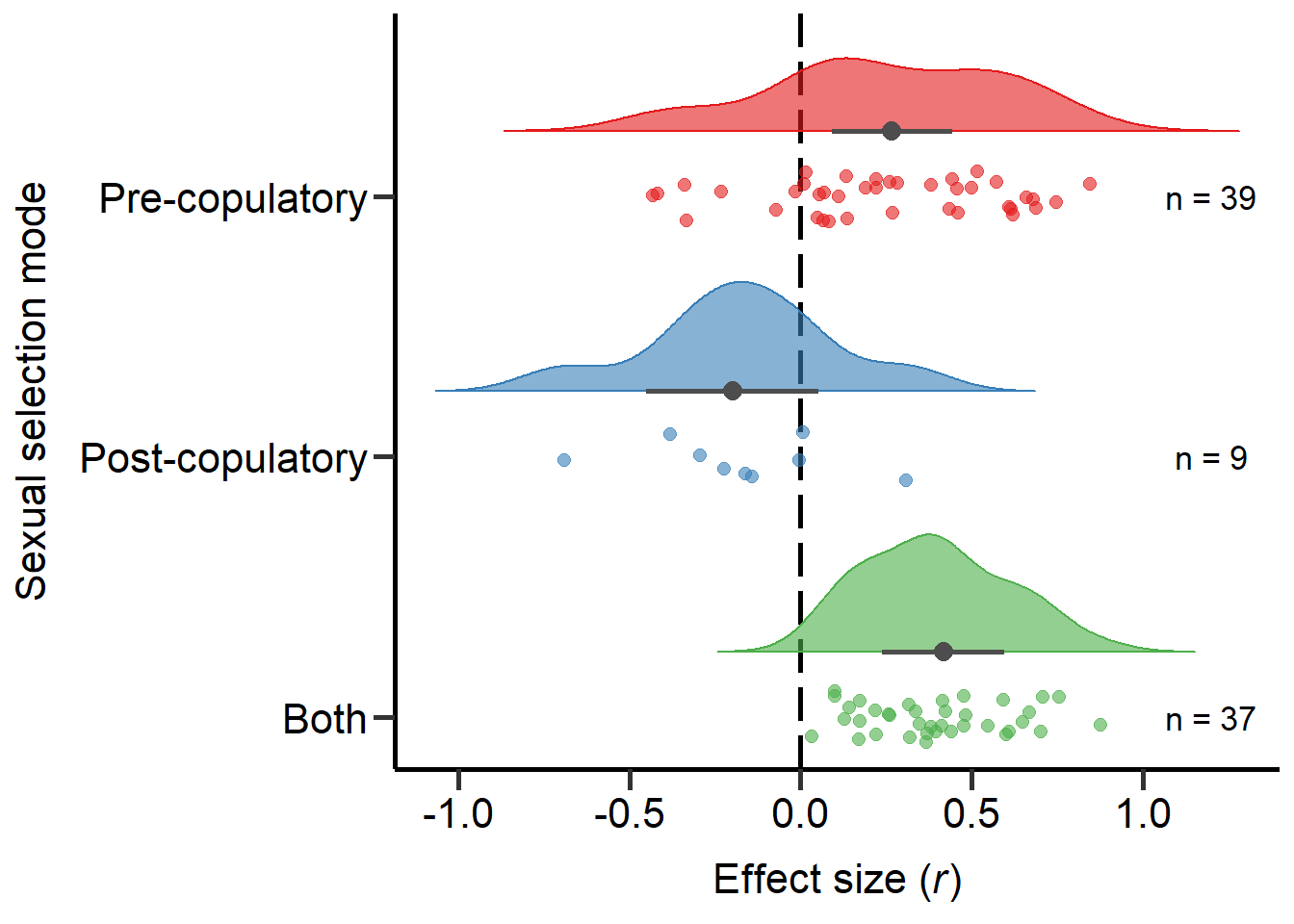

Figure 2: Raincloud plot of correlation coefficients between SSD and the modes of sexual selection proxies (i.e. pre-copulatory, post-copulatory or both) including sample sizes and estimates with 95%CI from phylogenetic model.

sessionInfo()

R version 4.2.0 (2022-04-22 ucrt)
Platform: x86_64-w64-mingw32/x64 (64-bit)
Running under: Windows 10 x64 (build 19045)

Matrix products: default

locale:
[1] LC_COLLATE=German_Germany.utf8  LC_CTYPE=German_Germany.utf8   
[3] LC_MONETARY=German_Germany.utf8 LC_NUMERIC=C                   
[5] LC_TIME=German_Germany.utf8    

attached base packages:
[1] stats     graphics  grDevices utils     datasets  methods   base     

other attached packages:
 [1] wesanderson_0.3.6   PupillometryR_0.0.4 rlang_1.0.6        
 [4] dplyr_1.1.0         cowplot_1.1.1       ggdist_3.2.1       
 [7] MCMCglmm_2.34       coda_0.19-4         RColorBrewer_1.1-3 
[10] ggplot2_3.4.1       data.table_1.14.8   multcomp_1.4-23    
[13] TH.data_1.1-1       survival_3.3-1      mvtnorm_1.1-3      
[16] psych_2.2.9         pwr_1.3-0           MASS_7.3-56        
[19] metafor_3.8-1       metadat_1.2-0       Matrix_1.5-3       
[22] matrixcalc_1.0-6    ape_5.7-1           workflowr_1.7.0    

loaded via a namespace (and not attached):
 [1] httr_1.4.5           sass_0.4.5           jsonlite_1.8.4      
 [4] splines_4.2.0        bslib_0.4.2          getPass_0.2-2       
 [7] distributional_0.3.1 highr_0.10           tensorA_0.36.2      
[10] yaml_2.3.7           pillar_1.8.1         lattice_0.20-45     
[13] glue_1.6.2           digest_0.6.31        promises_1.2.0.1    
[16] colorspace_2.1-0     sandwich_3.0-2       htmltools_0.5.4     
[19] httpuv_1.6.9         pkgconfig_2.0.3      corpcor_1.6.10      
[22] scales_1.2.1         processx_3.8.0       whisker_0.4.1       
[25] later_1.3.0          cubature_2.0.4.6     git2r_0.31.0        
[28] tibble_3.2.0         generics_0.1.3       farver_2.1.1        
[31] cachem_1.0.7         withr_2.5.0          cli_3.6.1           
[34] mnormt_2.1.1         magrittr_2.0.3       evaluate_0.20       
[37] ps_1.7.2             fs_1.6.1             fansi_1.0.4         
[40] nlme_3.1-157         tools_4.2.0          lifecycle_1.0.3     
[43] stringr_1.5.0        munsell_0.5.0        callr_3.7.3         
[46] compiler_4.2.0       jquerylib_0.1.4      grid_4.2.0          
[49] rstudioapi_0.14      labeling_0.4.2       rmarkdown_2.20      
[52] gtable_0.3.1         codetools_0.2-18     R6_2.5.1            
[55] zoo_1.8-11           knitr_1.42           fastmap_1.1.1       
[58] utf8_1.2.3           mathjaxr_1.6-0       rprojroot_2.0.3     
[61] stringi_1.7.12       parallel_4.2.0       Rcpp_1.0.10         
[64] vctrs_0.5.2          tidyselect_1.2.0     xfun_0.37