Pre-copulatory sexual selection predicts sexual size dimorphism: a meta-analysis of comparative studies
Main analyses
Lennart Winkler1, Robert P
Freckleton2, Tamas Szekely3, 4 &
Tim Janicke1,5
1Applied Zoology,
Technical University Dresden 2Department of
Zoology, University of Oxford, South Parks Road, Oxford OX1 3PS,
UK
3Milner Centre for Evolution, University of Bath,
Bath, UK84Department of Evolutionary Zoology and
Human Behaviour, University of Debrecen, Debrecen, Hungary
5Centre d’Écologie Fonctionnelle et Évolutive, UMR 5175,
CNRS, Université de Montpellier
Last updated: 2024-05-01
Checks: 6 1
Knit directory:
SSD_and_sexual_selection_2023/
This reproducible R Markdown analysis was created with workflowr (version 1.7.1). The Checks tab describes the reproducibility checks that were applied when the results were created. The Past versions tab lists the development history.
The R Markdown file has unstaged changes. To know which version of
the R Markdown file created these results, you’ll want to first commit
it to the Git repo. If you’re still working on the analysis, you can
ignore this warning. When you’re finished, you can run
wflow_publish to commit the R Markdown file and build the
HTML.
Great job! The global environment was empty. Objects defined in the global environment can affect the analysis in your R Markdown file in unknown ways. For reproduciblity it’s best to always run the code in an empty environment.
The command set.seed(20230430) was run prior to running
the code in the R Markdown file. Setting a seed ensures that any results
that rely on randomness, e.g. subsampling or permutations, are
reproducible.
Great job! Recording the operating system, R version, and package versions is critical for reproducibility.
Nice! There were no cached chunks for this analysis, so you can be confident that you successfully produced the results during this run.
Great job! Using relative paths to the files within your workflowr project makes it easier to run your code on other machines.
Great! You are using Git for version control. Tracking code development and connecting the code version to the results is critical for reproducibility.
The results in this page were generated with repository version b028b7d. See the Past versions tab to see a history of the changes made to the R Markdown and HTML files.
Note that you need to be careful to ensure that all relevant files for
the analysis have been committed to Git prior to generating the results
(you can use wflow_publish or
wflow_git_commit). workflowr only checks the R Markdown
file, but you know if there are other scripts or data files that it
depends on. Below is the status of the Git repository when the results
were generated:
Ignored files:
    Ignored:    .Rhistory

Untracked files:
    Untracked:  data/Data_SexSelSSD.csv
    Untracked:  data/Pyologeny_SexSelSSD.txt

Unstaged changes:
    Modified:   .Rprofile
    Modified:   .gitattributes
    Modified:   .gitignore
    Modified:   README.md
    Modified:   SSD_and_sexual_selection_2023.Rproj
    Modified:   _workflowr.yml
    Modified:   analysis/_site.yml
    Modified:   analysis/about.Rmd
    Modified:   analysis/index.Rmd
    Modified:   analysis/index2.Rmd
    Modified:   analysis/license.Rmd
    Modified:   code/README.md
    Modified:   data/README.md
    Deleted:    data/Supplement4_SexSelSSD_V01.csv
    Deleted:    data/Supplement6_SexSelSSD_V01.txt
    Modified:   output/README.md
Note that any generated files, e.g. HTML, png, CSS, etc., are not included in this status report because it is ok for generated content to have uncommitted changes.
These are the previous versions of the repository in which changes were
made to the R Markdown (analysis/index.Rmd) and HTML
(docs/index.html) files. If you’ve configured a remote Git
repository (see ?wflow_git_remote), click on the hyperlinks
in the table below to view the files as they were in that past version.
| File | Version | Author | Date | Message |
|---|---|---|---|---|
| html | b028b7d | LennartWinkler | 2023-05-24 | Build site. |
| Rmd | c1d3311 | LennartWinkler | 2023-05-24 | wflow_publish(all = T) |
| html | 71d667c | LennartWinkler | 2023-05-03 | Build site. |
| Rmd | 378a58c | LennartWinkler | 2023-05-03 | wflow_publish(republish = TRUE, all = T) |
| html | 085f45f | LennartWinkler | 2023-05-03 | Build site. |
| Rmd | 85c143e | LennartWinkler | 2023-05-03 | update |
| html | 8edd942 | LennartWinkler | 2023-05-01 | Build site. |
| Rmd | d131cd9 | LennartWinkler | 2023-05-01 | wflow_publish(republish = TRUE, all = T) |
| Rmd | 57ca562 | LennartWinkler | 2023-04-30 | update |
| html | 054a12b | LennartWinkler | 2023-04-30 | Build site. |
| Rmd | 1a5561c | LennartWinkler | 2023-04-30 | wflow_publish(all = T) |
| Rmd | 4482c88 | LennartWinkler | 2023-04-30 | Start workflowr project. |
Supplementary material reporting R code for the manuscript ‘Pre-copulatory sexual selection predicts sexual size dimorphism: a meta-analysis of comparative studies’. Additional analyses excluding studies that did not control for phylogenetic non-independence (Supplement 2) can be found at: https://https://lennartwinkler.github.io/SSD_and_sexual_selection_2023/index2.html # Load and prepare data Before we started the analyses, we loaded all necessary packages and data.
rm(list = ls()) # Clear work environment

# Load R-packages ####
list_of_packages=cbind('ape','matrixcalc','metafor','Matrix','MASS','pwr','psych','multcomp','data.table','ggplot2','RColorBrewer','MCMCglmm','ggdist','cowplot','PupillometryR','dplyr','wesanderson','gridExtra')
lapply(list_of_packages, require, character.only = TRUE)

# Load data set ####
MetaData <- read.csv("./data/Data_SexSelSSD.csv", sep=";", header=TRUE) # Load data set

N_Studies <- length(summary(as.factor(MetaData$Study_ID))) # Number of included primary studies

Tree<- read.tree("./data/Pyologeny_SexSelSSD.txt") # Load phylogenetic tree

# Prune phylogenetic tree
MetaData_Class_Data <- unique(MetaData$Class)
Tree_Class<-drop.tip(Tree, Tree$tip.label[-na.omit(match(MetaData_Class_Data, Tree$tip.label))])
forcedC_Moderators <- as.matrix(forceSymmetric(vcv(Tree_Class, corr=TRUE)))

# Order moderator levels
MetaData$SexSel_Episode=as.factor(MetaData$SexSel_Episode)
MetaData$SexSel_Episode=relevel(MetaData$SexSel_Episode,c("post-copulatory"))
MetaData$SexSel_Episode=relevel(MetaData$SexSel_Episode,c("pre-copulatory"))
MetaData$Class=as.factor(MetaData$Class)
MetaData$z=as.numeric(MetaData$z)

# Set figure theme and colors
theme=theme(panel.border = element_blank(),
            panel.background = element_blank(),
            panel.grid.major = element_blank(),
            panel.grid.minor = element_blank(),
            legend.position = c(0.2,0.5),
            legend.title = element_blank(),
            legend.text = element_text(colour="black", size=12),
            axis.line.x = element_line(colour = "black", linewidth = 1),
            axis.line.y = element_line(colour = "black", linewidth = 1),
            axis.text.x = element_text(face="plain", color="black", size=12, angle=0),
            axis.text.y = element_text(face="plain", color="black", size=12, angle=0),
            axis.title.x = element_text(size=14,face="plain", margin = margin(r=0,10,0,0)),
            axis.title.y = element_text(size=14,face="plain", margin = margin(r=10,0,0,0)),
            axis.ticks = element_line(linewidth = 1),
            axis.ticks.length = unit(.3, "cm"))

colpal=c('#003d6cff','#0c7accff','#5a9c97ff')

colpal2=brewer.pal(7, 'Dark2')
colpal3=brewer.pal(10, 'BrBG')
colpal4=c("grey50","grey65")
colpal5=c("#8C2D04","#CC4C02", "#EC7014", "#FE9929", "#FEC44F","#A8DDB5","#A8DDB5", "#7BCCC4", "#4EB3D3", "#2B8CBE", "#08589E")
colpal6=c("#8C2D04","#CC4C02", "#EC7014", "#FE9929", "#FEC44F","#A8DDB5", "#7BCCC4", "#4EB3D3", "#2B8CBE", "#08589E")
Meta_col=c('#5a9c97ff','#0c7accff','#003d6cff','black')
Global models
We addressed the question if increasing sexual selection correlated with an increasingly male-biased SSD. For this we ran a global model including an observation-level index and the study identifier as random termson correlation coefficients that were positive if increasing sexual selection correlated with an increasingly male-biased SSD, but negative if increasing sexual selection correlated with an increasingly female-biased SSD. First, we ran a global model including the phylogeny:
Model_REML_Null         = rma.mv(r ~ 1, V=Var_r, data = MetaData, random = c(~ 1 | Study_ID,~ 1 | Index, ~ 1 | Class), R = list(Class = forcedC_Moderators), method = "REML")
summary(Model_REML_Null)
Multivariate Meta-Analysis Model (k = 122; method: REML)

  logLik  Deviance       AIC       BIC      AICc
-23.7816   47.5632   55.5632   66.7464   55.9080

Variance Components:

            estim    sqrt  nlvls  fixed    factor    R
sigma^2.1  0.0205  0.1431     73     no  Study_ID   no
sigma^2.2  0.0484  0.2199    122     no     Index   no
sigma^2.3  0.0130  0.1140     11     no     Class  yes

Test for Heterogeneity:
Q(df = 121) = 1559.2739, p-val < .0001

Model Results:

estimate      se    zval    pval   ci.lb   ci.ub
  0.2498  0.0733  3.4095  0.0007  0.1062  0.3934  ***

---
Signif. codes:  0 '***' 0.001 '**' 0.01 '*' 0.05 '.' 0.1 ' ' 1
Second, we ran a global model without the phylogeny:
Model_cREML_Null         = rma.mv(r ~ 1, V=Var_r, data = MetaData, random = c(~ 1 | Study_ID,~ 1 | Index), method = "REML")
summary(Model_cREML_Null)
Multivariate Meta-Analysis Model (k = 122; method: REML)

  logLik  Deviance       AIC       BIC      AICc
-25.1523   50.3047   56.3047   64.6921   56.5098

Variance Components:

            estim    sqrt  nlvls  fixed    factor
sigma^2.1  0.0316  0.1777     73     no  Study_ID
sigma^2.2  0.0460  0.2144    122     no     Index

Test for Heterogeneity:
Q(df = 121) = 1559.2739, p-val < .0001

Model Results:

estimate      se    zval    pval   ci.lb   ci.ub
  0.2670  0.0321  8.3255  <.0001  0.2042  0.3299  ***

---
Signif. codes:  0 '***' 0.001 '**' 0.01 '*' 0.05 '.' 0.1 ' ' 1
Moderator tests for phylogenetic models
Next, we ran a series of models that test the effect of different moderators. Again we started with models including the phylogeny.
Sexual selection episode
The first model explores the effect of the different episodes of sexual selection (i.e. pre-copulatory, post-copulatory or both):
MetaData$SexSel_Episode=relevel(MetaData$SexSel_Episode,c("pre-copulatory"))
Model_REML_by_SexSelEpisode = rma.mv(r ~ factor(SexSel_Episode), V=Var_r, data = MetaData, random = c(~ 1 | Study_ID,~ 1 | Index, ~ 1 | Class), R = list(Class = forcedC_Moderators), method = "REML")
summary(Model_REML_by_SexSelEpisode)
Multivariate Meta-Analysis Model (k = 122; method: REML)

  logLik  Deviance       AIC       BIC      AICc
 -8.4861   16.9722   28.9722   45.6469   29.7222

Variance Components:

            estim    sqrt  nlvls  fixed    factor    R
sigma^2.1  0.0167  0.1293     73     no  Study_ID   no
sigma^2.2  0.0338  0.1839    122     no     Index   no
sigma^2.3  0.0125  0.1119     11     no     Class  yes

Test for Residual Heterogeneity:
QE(df = 119) = 1337.5244, p-val < .0001

Test of Moderators (coefficients 2:3):
QM(df = 2) = 35.8143, p-val < .0001

Model Results:

                                       estimate      se     zval    pval
intrcpt                                  0.2494  0.0755   3.3009  0.0010
factor(SexSel_Episode)post-copulatory   -0.3476  0.0816  -4.2614  <.0001
factor(SexSel_Episode)both               0.1415  0.0531   2.6632  0.0077
                                         ci.lb    ci.ub
intrcpt                                 0.1013   0.3974  ***
factor(SexSel_Episode)post-copulatory  -0.5075  -0.1877  ***
factor(SexSel_Episode)both              0.0374   0.2456   **

---
Signif. codes:  0 '***' 0.001 '**' 0.01 '*' 0.05 '.' 0.1 ' ' 1
We then re-leveled the model for post-hoc comparisons:
MetaData$SexSel_Episode=relevel(MetaData$SexSel_Episode,c("post-copulatory"))
Model_REML_by_SexSelEpisode2 = rma.mv(r ~ factor(SexSel_Episode), V=Var_r, data = MetaData, random = c(~ 1 | Study_ID,~ 1 | Index, ~ 1 | Class), R = list(Class = forcedC_Moderators), method = "REML")
summary(Model_REML_by_SexSelEpisode2)

MetaData$SexSel_Episode=relevel(MetaData$SexSel_Episode,c("both"))
Model_REML_by_SexSelEpisode3 = rma.mv(r ~ factor(SexSel_Episode), V=Var_r, data = MetaData, random = c(~ 1 | Study_ID,~ 1 | Index, ~ 1 | Class), R = list(Class = forcedC_Moderators), method = "REML")
summary(Model_REML_by_SexSelEpisode3)
Finally, we computed FDR corrected p-values:
tab1=as.data.frame(round(p.adjust(c(.0001, 0.3004, .0001), method = 'fdr'),digit=3),row.names=cbind("Pre-copulatory","Post-copulatory","Both"))
colnames(tab1)<-cbind('P-value')
tab1
P-value
Pre-copulatory 0.0
Post-copulatory 0.3
Both 0.0Plot sexual selection mode (Figure 3)
Here we plot the sexual selection mode moderator:
MetaData$SexSel_Episode=factor(MetaData$SexSel_Episode, levels = c("both","post-copulatory" ,"pre-copulatory"))

ggplot(MetaData, aes(x=SexSel_Episode, y=r, fill = SexSel_Episode, colour = SexSel_Episode)) +
  geom_hline(yintercept=0, linetype="longdash", color = "black", linewidth=1)+
  geom_flat_violin(position = position_nudge(x = 0.25, y = 0),adjust =1, trim = F,alpha=0.6)+
  geom_point(position = position_jitter(width = .1), size = 2.5,alpha=0.6,stroke=0,shape=19)+
  geom_segment(inherit.aes = F,mapping = aes(y=Model_REML_by_SexSelEpisode$ci.lb[1], x=3.25, xend= 3.25, yend= Model_REML_by_SexSelEpisode$ci.ub[1]), alpha=1,linewidth=1,color='black')+
  geom_segment(inherit.aes = F,mapping = aes(y=Model_REML_by_SexSelEpisode2$ci.lb[1], x=2.25, xend= 2.25, yend= Model_REML_by_SexSelEpisode2$ci.ub[1]), alpha=1,linewidth=1,color='black')+
  geom_segment(inherit.aes = F,mapping = aes(y=Model_REML_by_SexSelEpisode3$ci.lb[1], x=1.25, xend= 1.25, yend= Model_REML_by_SexSelEpisode3$ci.ub[1]), alpha=1,linewidth=1,color='black')+
  geom_point(inherit.aes = F,mapping = aes(y=Model_REML_by_SexSelEpisode$b[1,1], x=3.25), size = 3.5,alpha=1,stroke=1,shape=21,fill='grey50',color='black')+
  geom_point(inherit.aes = F,mapping = aes(y=Model_REML_by_SexSelEpisode2$b[1,1], x=2.25), size = 3.5,alpha=1,stroke=1,shape=21,fill='white',color='black')+
  geom_point(inherit.aes = F,mapping = aes(y=Model_REML_by_SexSelEpisode3$b[1,1], x=1.25), size = 3.5,alpha=1,stroke=1,shape=21,fill='black',color='black')+
  ylab(expression(paste("Effect size (", italic("r"),')')))+xlab('Sexual selection episode')+coord_flip()+guides(fill = FALSE, colour = FALSE) +
  scale_color_manual(values =colpal)+
  scale_fill_manual(values =colpal)+
  scale_x_discrete(labels=c("Pre- and      \n post-copulatory","Post-copulatory" ,"Pre-copulatory"),expand=c(.1,0))+
  annotate("text", x=1, y=1.2, label= "n = 48",size=4.5) +
  annotate("text", x=2, y=1.2, label= "n = 19",size=4.5) +
  annotate("text", x=3, y=1.2, label= "n = 55",size=4.5) + theme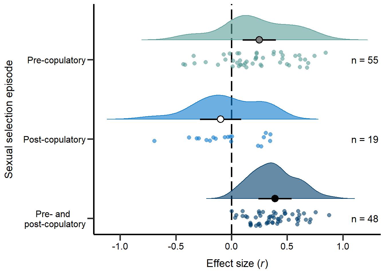
Figure 3: Raincloud plot of correlation coefficients between SSD and the modes of sexual selection proxies (i.e. pre-copulatory, post-copulatory or both) including sample sizes and estimates with 95%CI from phylogenetic model.
| Version | Author | Date |
|---|---|---|
| 8edd942 | LennartWinkler | 2023-05-01 |
Sexual selection category
Next we explored the effect of the sexual selection category (i.e. density, mating system, operational sex ratio (OSR), post-mating competition, pre-mating competition, trait-based, other):
MetaData$SexSel_Category=as.factor(MetaData$SexSel_Category)
MetaData$SexSel_Category=relevel(MetaData$SexSel_Category,c("Postmating competition"))
Model_REML_by_SexSelCat = rma.mv(r ~ factor(SexSel_Category), V=Var_r, data = MetaData, random = c(~ 1 | Study_ID,~ 1 | Index, ~ 1 | Class), R = list(Class = forcedC_Moderators), method = "REML")
summary(Model_REML_by_SexSelCat)
Multivariate Meta-Analysis Model (k = 122; method: REML)

  logLik  Deviance       AIC       BIC      AICc
  5.8584  -11.7168    8.2832   35.7326   10.3986

Variance Components:

            estim    sqrt  nlvls  fixed    factor    R
sigma^2.1  0.0209  0.1446     73     no  Study_ID   no
sigma^2.2  0.0181  0.1345    122     no     Index   no
sigma^2.3  0.0123  0.1109     11     no     Class  yes

Test for Residual Heterogeneity:
QE(df = 115) = 916.8832, p-val < .0001

Test of Moderators (coefficients 2:7):
QM(df = 6) = 83.7711, p-val < .0001

Model Results:

                                              estimate      se     zval    pval
intrcpt                                        -0.1218  0.0915  -1.3305  0.1834
factor(SexSel_Category)Density                  0.3310  0.1209   2.7376  0.0062
factor(SexSel_Category)Mating system            0.4737  0.0793   5.9704  <.0001
factor(SexSel_Category)OSR                      0.7397  0.1285   5.7572  <.0001
factor(SexSel_Category)Other                    0.4501  0.0933   4.8255  <.0001
factor(SexSel_Category)Premating competition    0.4601  0.0819   5.6138  <.0001
factor(SexSel_Category)Trait-based              0.1059  0.0891   1.1887  0.2346
                                                ci.lb   ci.ub
intrcpt                                       -0.3012  0.0576
factor(SexSel_Category)Density                 0.0940  0.5679   **
factor(SexSel_Category)Mating system           0.3182  0.6292  ***
factor(SexSel_Category)OSR                     0.4879  0.9915  ***
factor(SexSel_Category)Other                   0.2673  0.6329  ***
factor(SexSel_Category)Premating competition   0.2994  0.6207  ***
factor(SexSel_Category)Trait-based            -0.0687  0.2805

---
Signif. codes:  0 '***' 0.001 '**' 0.01 '*' 0.05 '.' 0.1 ' ' 1
We then re-leveled the model for post-hoc comparisons:
MetaData$SexSel_Category=relevel(MetaData$SexSel_Category,c("Trait-based"))
Model_REML_by_SexSelCat2 = rma.mv(r ~ factor(SexSel_Category), V=Var_r, data = MetaData, random = c(~ 1 | Study_ID,~ 1 | Index, ~ 1 | Class), R = list(Class = forcedC_Moderators), method = "REML")
summary(Model_REML_by_SexSelCat2)

MetaData$SexSel_Category=relevel(MetaData$SexSel_Category,c("Density"))
Model_REML_by_SexSelCat3 = rma.mv(r ~ factor(SexSel_Category), V=Var_r, data = MetaData, random = c(~ 1 | Study_ID,~ 1 | Index, ~ 1 | Class), R = list(Class = forcedC_Moderators), method = "REML")
summary(Model_REML_by_SexSelCat3)

MetaData$SexSel_Category=relevel(MetaData$SexSel_Category,c("Premating competition"))
Model_REML_by_SexSelCat4 = rma.mv(r ~ factor(SexSel_Category), V=Var_r, data = MetaData, random = c(~ 1 | Study_ID,~ 1 | Index, ~ 1 | Class), R = list(Class = forcedC_Moderators), method = "REML")
summary(Model_REML_by_SexSelCat4)

MetaData$SexSel_Category=relevel(MetaData$SexSel_Category,c("Mating system"))
Model_REML_by_SexSelCat5 = rma.mv(r ~ factor(SexSel_Category), V=Var_r, data = MetaData, random = c(~ 1 | Study_ID,~ 1 | Index, ~ 1 | Class), R = list(Class = forcedC_Moderators), method = "REML")
summary(Model_REML_by_SexSelCat5)

MetaData$SexSel_Category=relevel(MetaData$SexSel_Category,c("OSR"))
Model_REML_by_SexSelCat6 = rma.mv(r ~ factor(SexSel_Category), V=Var_r, data = MetaData, random = c(~ 1 | Study_ID,~ 1 | Index, ~ 1 | Class), R = list(Class = forcedC_Moderators), method = "REML")
summary(Model_REML_by_SexSelCat6)

MetaData$SexSel_Category=relevel(MetaData$SexSel_Category,c("Other"))
Model_REML_by_SexSelCat7 = rma.mv(r ~ factor(SexSel_Category), V=Var_r, data = MetaData, random = c(~ 1 | Study_ID,~ 1 | Index, ~ 1 | Class), R = list(Class = forcedC_Moderators), method = "REML")
summary(Model_REML_by_SexSelCat7)
Finally, we computed FDR corrected p-values:
tab2=as.data.frame(round(p.adjust(c(0.1834, 0.8561, 0.0826, .0001, .0001, .0001, 0.0002), method = 'fdr'),digit=3),row.names=cbind("Postmating competition","Trait-based","Density",'Premating competition',"Mating system","OSR","Other"))
colnames(tab2)<-cbind('P-value')
tab2
P-value
Postmating competition 0.214
Trait-based 0.856
Density 0.116
Premating competition 0.000
Mating system 0.000
OSR 0.000
Other 0.000Plot sexual selection category (Figure S1)
Here we plot the sexual selection category moderator:
MetaData$SexSel_Category=factor(MetaData$SexSel_Category, levels = rev(c( "Postmating competition","Trait-based" ,"Density","Premating competition" ,"Mating system" , "OSR", "Other")))

ggplot(MetaData, aes(x=SexSel_Category, y=r, fill = SexSel_Category, colour = SexSel_Category)) +
  geom_hline(yintercept=0, linetype="longdash", color = "black", linewidth=1)+
  geom_flat_violin(position = position_nudge(x = 0.25, y = 0),adjust =1, trim = F,alpha=0.6)+
  geom_point(position = position_jitter(width = .1), size = 2.5,alpha=0.6,stroke=0,shape=19)+
  geom_point(inherit.aes = F,mapping = aes(y=Model_REML_by_SexSelCat$b[1,1], x=7.25), size = 3.5,alpha=1,stroke=0,shape=19,color='grey30')+
  geom_point(inherit.aes = F,mapping = aes(y=Model_REML_by_SexSelCat2$b[1,1], x=6.25), size = 3.5,alpha=1,stroke=0,shape=19,color='grey30')+
  geom_point(inherit.aes = F,mapping = aes(y=Model_REML_by_SexSelCat3$b[1,1], x=5.25), size = 3.5,alpha=1,stroke=0,shape=19,color='grey30')+
  geom_point(inherit.aes = F,mapping = aes(y=Model_REML_by_SexSelCat4$b[1,1], x=4.25), size = 3.5,alpha=1,stroke=0,shape=19,color='grey30')+
  geom_point(inherit.aes = F,mapping = aes(y=Model_REML_by_SexSelCat5$b[1,1], x=3.25), size = 3.5,alpha=1,stroke=0,shape=19,color='grey30')+
  geom_point(inherit.aes = F,mapping = aes(y=Model_REML_by_SexSelCat6$b[1,1], x=2.25), size = 3.5,alpha=1,stroke=0,shape=19,color='grey30')+
  geom_point(inherit.aes = F,mapping = aes(y=Model_REML_by_SexSelCat7$b[1,1], x=1.25), size = 3.5,alpha=1,stroke=0,shape=19,color='grey30')+
  geom_segment(inherit.aes = F,mapping = aes(y=Model_REML_by_SexSelCat$ci.lb[1], x=7.25, xend= 7.25, yend= Model_REML_by_SexSelCat$ci.ub[1]), alpha=1,linewidth=1,color='grey30')+
  geom_segment(inherit.aes = F,mapping = aes(y=Model_REML_by_SexSelCat2$ci.lb[1], x=6.25, xend= 6.25, yend= Model_REML_by_SexSelCat2$ci.ub[1]), alpha=1,linewidth=1,color='grey30')+
  geom_segment(inherit.aes = F,mapping = aes(y=Model_REML_by_SexSelCat3$ci.lb[1], x=5.25, xend= 5.25, yend= Model_REML_by_SexSelCat3$ci.ub[1]), alpha=1,linewidth=1,color='grey30')+
  geom_segment(inherit.aes = F,mapping = aes(y=Model_REML_by_SexSelCat4$ci.lb[1], x=4.25, xend= 4.25, yend= Model_REML_by_SexSelCat4$ci.ub[1]), alpha=1,linewidth=1,color='grey30')+
  geom_segment(inherit.aes = F,mapping = aes(y=Model_REML_by_SexSelCat5$ci.lb[1], x=3.25, xend= 3.25, yend= Model_REML_by_SexSelCat5$ci.ub[1]), alpha=1,linewidth=1,color='grey30')+
  geom_segment(inherit.aes = F,mapping = aes(y=Model_REML_by_SexSelCat6$ci.lb[1], x=2.25, xend= 2.25, yend= Model_REML_by_SexSelCat6$ci.ub[1]), alpha=1,linewidth=1,color='grey30')+
  geom_segment(inherit.aes = F,mapping = aes(y=Model_REML_by_SexSelCat7$ci.lb[1], x=1.25, xend= 1.25, yend= Model_REML_by_SexSelCat7$ci.ub[1]), alpha=1,linewidth=1,color='grey30')+
  ylab(expression(paste("Effect size (", italic("r"),')')))+xlab('Sexual selection category')+coord_flip()+guides(fill = FALSE, colour = FALSE) +
  scale_color_manual(values =colpal2)+
  scale_fill_manual(values =colpal2)+
  scale_x_discrete(labels=rev(c( "Post-mating\ncompetition","Trait-based" ,"Population\ndensity","Pre-mating\ncompetition" ,"Mating\nsystem" , "Sex ratio", "Other")),expand=c(.1,0))+
  annotate("text", x=7, y=1.2, label= "n = 19",size=4.5) +
  annotate("text", x=6, y=1.2, label= "n = 17",size=4.5) +
  annotate("text", x=5, y=1.2, label= "n = 5",size=4.5) +
  annotate("text", x=4, y=1.2, label= "n = 22",size=4.5) +
  annotate("text", x=3, y=1.2, label= "n = 36",size=4.5) +
  annotate("text", x=2, y=1.2, label= "n = 6",size=4.5) +
  annotate("text", x=1, y=1.2, label= "n = 17",size=4.5) + theme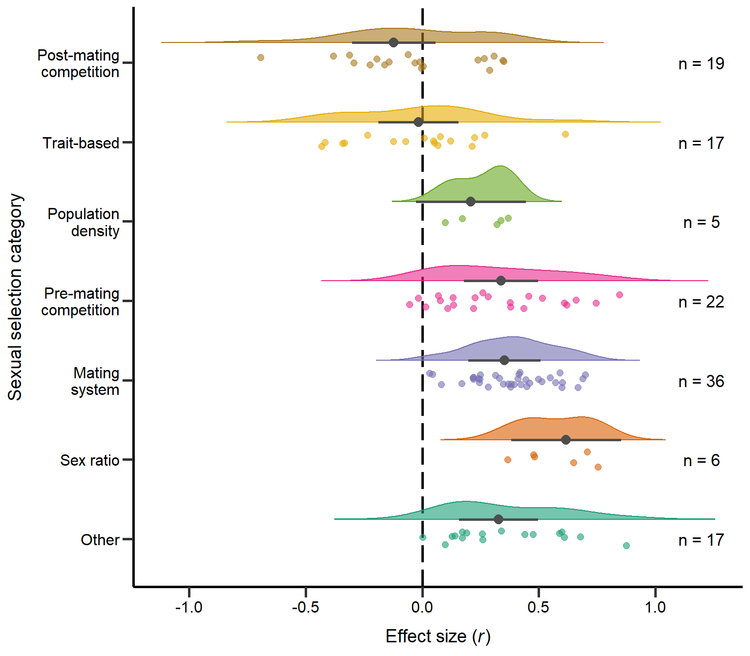
Figure S1: Raincloud plot of correlation coefficients between SSD and different sexual selection categories including sample sizes and estimates with 95%CI from phylogenetic model.
| Version | Author | Date |
|---|---|---|
| 8edd942 | LennartWinkler | 2023-05-01 |
Type of SSD measure
Next we explored the effect of the type of SSD measure (i.e. body mass or size):
MetaData$SSD_Proxy=as.factor(MetaData$SSD_Proxy)
MetaData$SSD_Proxy=relevel(MetaData$SSD_Proxy,c("Body mass"))
Model_REML_by_SSDMeasure = rma.mv(r ~ SSD_Proxy, V=Var_r, data = MetaData, random = c(~ 1 | Study_ID,~ 1 | Index, ~ 1 | Class), R = list(Class = forcedC_Moderators), method = "REML")
summary(Model_REML_by_SSDMeasure)
Multivariate Meta-Analysis Model (k = 120; method: REML)

  logLik  Deviance       AIC       BIC      AICc
-23.6341   47.2682   57.2682   71.1216   57.8039

Variance Components:

            estim    sqrt  nlvls  fixed    factor    R
sigma^2.1  0.0235  0.1534     72     no  Study_ID   no
sigma^2.2  0.0485  0.2203    120     no     Index   no
sigma^2.3  0.0047  0.0688     11     no     Class  yes

Test for Residual Heterogeneity:
QE(df = 118) = 1511.0606, p-val < .0001

Test of Moderators (coefficient 2):
QM(df = 1) = 2.3553, p-val = 0.1249

Model Results:

                    estimate      se     zval    pval    ci.lb   ci.ub
intrcpt               0.3292  0.0715   4.6056  <.0001   0.1891  0.4693  ***
SSD_ProxyBody size   -0.1015  0.0662  -1.5347  0.1249  -0.2312  0.0281

---
Signif. codes:  0 '***' 0.001 '**' 0.01 '*' 0.05 '.' 0.1 ' ' 1
We then re-leveled the model for post-hoc comparisons:
MetaData$SSD_Proxy=relevel(MetaData$SSD_Proxy,c("Body size"))
Model_REML_by_SSDMeasure2 = rma.mv(r ~ SSD_Proxy, V=Var_r, data = MetaData, random = c(~ 1 | Study_ID,~ 1 | Index, ~ 1 | Class), R = list(Class = forcedC_Moderators), method = "REML")
summary(Model_REML_by_SSDMeasure2)
Finally, we computed FDR corrected p-values:
tab3=as.data.frame(round(p.adjust(c(.0001, .0001), method = 'fdr'),digit=3),row.names=cbind("Body mass","Body size"))
colnames(tab3)<-cbind('P-value')
tab3
P-value
Body mass 0
Body size 0Plot Type of SSD measure (Figure S2A)
Here we plot the type of SSD measure moderator:
MetaData_NAProxy=MetaData[!is.na(MetaData$SSD_Proxy),]
MetaData_NAProxy$SSD_Proxy=as.factor(MetaData_NAProxy$SSD_Proxy)
MetaData_NAProxy$SSD_Proxy=relevel(MetaData_NAProxy$SSD_Proxy,c("Body size"))

ggplot(MetaData_NAProxy, aes(x=SSD_Proxy, y=r, fill = SSD_Proxy, colour = SSD_Proxy)) +
  geom_hline(yintercept=0, linetype="longdash", color = "black", linewidth=1)+
  geom_flat_violin(position = position_nudge(x = 0.25, y = 0),adjust =1, trim = F,alpha=0.6)+
  geom_point(position = position_jitter(width = .1), size = 2.5,alpha=0.6,stroke=0,shape=19)+
  geom_point(inherit.aes = F,mapping = aes(y=Model_REML_by_SSDMeasure$b[1,1], x=2.25), size = 3.5,alpha=1,stroke=0,shape=19,color='grey30')+
  geom_point(inherit.aes = F,mapping = aes(y=Model_REML_by_SSDMeasure2$b[1,1], x=1.25), size = 3.5,alpha=1,stroke=0,shape=19,color='grey30')+
  geom_segment(inherit.aes = F,mapping = aes(y=Model_REML_by_SSDMeasure$ci.lb[1], x=2.25, xend= 2.25, yend= Model_REML_by_SSDMeasure$ci.ub[1]), alpha=1,linewidth=1,color='grey30')+
  geom_segment(inherit.aes = F,mapping = aes(y=Model_REML_by_SSDMeasure2$ci.lb[1], x=1.25, xend= 1.25, yend= Model_REML_by_SSDMeasure2$ci.ub[1]), alpha=1,linewidth=1,color='grey30')+
  ylab(expression(paste("Effect size (", italic("r"),')')))+xlab('SSD proxy')+coord_flip()+guides(fill = FALSE, colour = FALSE) +
  scale_color_manual(values =colpal4)+
  scale_fill_manual(values =colpal4)+
  scale_x_discrete(labels=rev(c("Body \nmass ","Body \n size ")),expand=c(.15,0))+
  annotate("text", x=2, y=1.1, label= "n = 57",size=3.5) +
  annotate("text", x=1, y=1.1, label= "n = 63",size=3.5)  + theme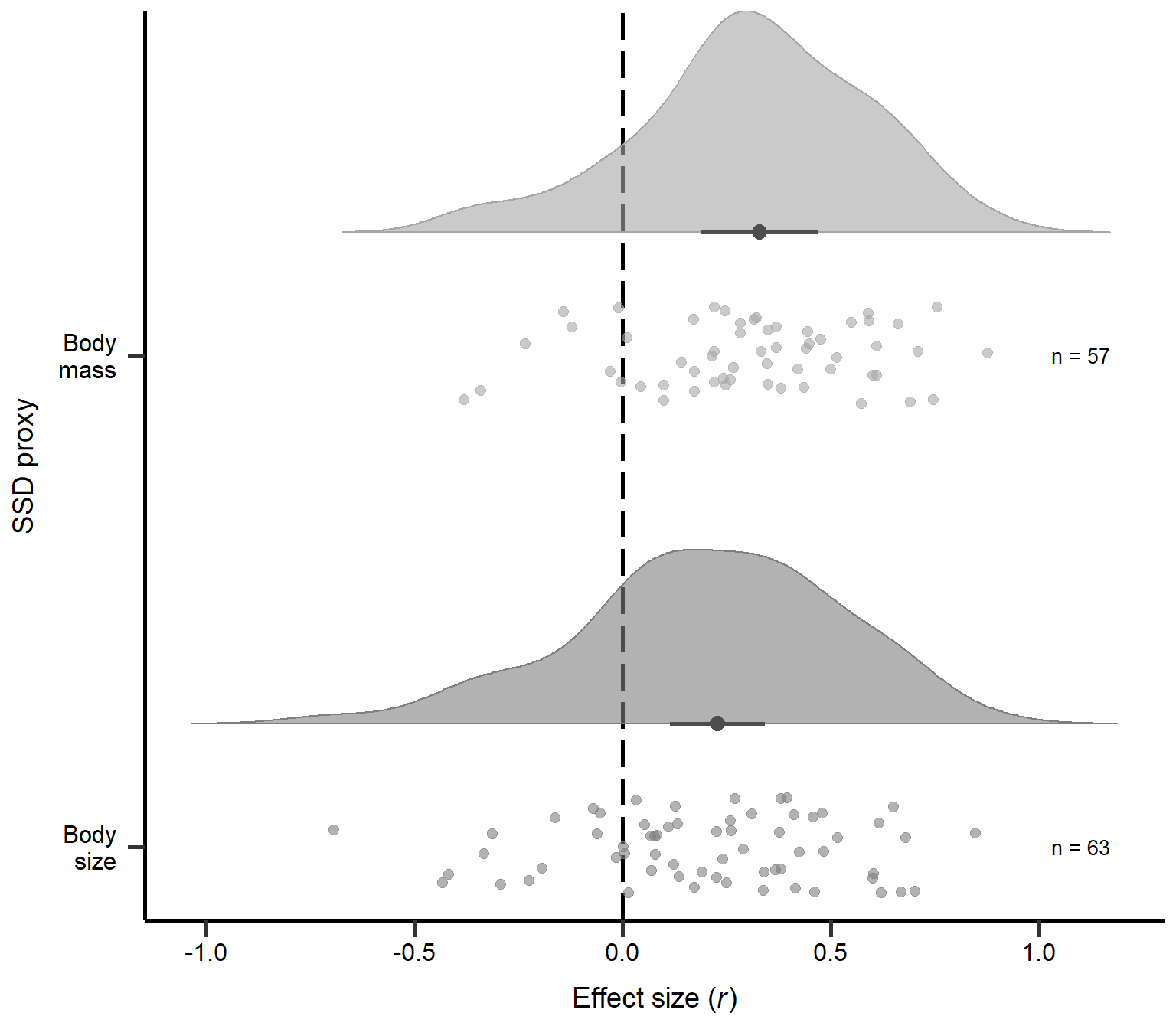
Figure S2A: Raincloud plot of correlation coefficients for different types of SSD measures (i.e. body mass or size) including sample sizes and estimates with 95% CI from phylogenetic model.
SSD measure controlled for body size?
Next we explored the effect if the primary study controlled the SSD for body size (i.e. uncontrolled or controlled):
MetaData$BodySizeControlled=as.factor(MetaData$BodySizeControlled)
MetaData$BodySizeControlled=relevel(MetaData$BodySizeControlled,c("No"))
Model_REML_by_BodySizeCont = rma.mv(r ~ BodySizeControlled, V=Var_r, data = MetaData, random = c(~ 1 | Study_ID,~ 1 | Index, ~ 1 | Class), R = list(Class = forcedC_Moderators), method = "REML")
summary(Model_REML_by_BodySizeCont)
Multivariate Meta-Analysis Model (k = 122; method: REML)

  logLik  Deviance       AIC       BIC      AICc
-23.6694   47.3387   57.3387   71.2762   57.8650

Variance Components:

            estim    sqrt  nlvls  fixed    factor    R
sigma^2.1  0.0210  0.1449     73     no  Study_ID   no
sigma^2.2  0.0483  0.2199    122     no     Index   no
sigma^2.3  0.0120  0.1094     11     no     Class  yes

Test for Residual Heterogeneity:
QE(df = 120) = 1555.0586, p-val < .0001

Test of Moderators (coefficient 2):
QM(df = 1) = 0.6071, p-val = 0.4359

Model Results:

                       estimate      se     zval    pval    ci.lb   ci.ub
intrcpt                  0.2629  0.0732   3.5909  0.0003   0.1194  0.4063  ***
BodySizeControlledYes   -0.0674  0.0865  -0.7792  0.4359  -0.2368  0.1021

---
Signif. codes:  0 '***' 0.001 '**' 0.01 '*' 0.05 '.' 0.1 ' ' 1
We then re-leveled the model for post-hoc comparisons:
MetaData$BodySizeControlled=relevel(MetaData$BodySizeControlled,c("Yes"))
Model_REML_by_BodySizeCont2 = rma.mv(r ~ BodySizeControlled, V=Var_r, data = MetaData, random = c(~ 1 | Study_ID,~ 1 | Index, ~ 1 | Class), R = list(Class = forcedC_Moderators), method = "REML")
summary(Model_REML_by_BodySizeCont2)
Finally, we computed FDR corrected p-values:
tab4=as.data.frame(round(p.adjust(c(.0001, 0.0517), method = 'fdr'),digit=3),row.names=cbind("uncontrolled","controlled"))
colnames(tab4)<-cbind('P-value')
tab4
P-value
uncontrolled 0.000
controlled 0.052Plot: SSD measure controlled for body size? (Figure S2B)
Here we plot effect sizes if type of SSD measure controlled for body size:
MetaData$BodySizeControlled=as.factor(MetaData$BodySizeControlled)
MetaData$BodySizeControlled=relevel(MetaData$BodySizeControlled,c("Yes"))

ggplot(MetaData, aes(x=BodySizeControlled, y=r, fill = BodySizeControlled, colour = BodySizeControlled)) +
  geom_hline(yintercept=0, linetype="longdash", color = "black", linewidth=1)+
  geom_flat_violin(position = position_nudge(x = 0.25, y = 0),adjust =1, trim = F,alpha=0.6)+
  geom_point(position = position_jitter(width = .1), size = 2.5,alpha=0.6,stroke=0,shape=19)+
  geom_point(inherit.aes = F,mapping = aes(y=Model_REML_by_BodySizeCont$b[1,1], x=2.25), size = 3.5,alpha=1,stroke=0,shape=19,color='grey30')+
  geom_point(inherit.aes = F,mapping = aes(y=Model_REML_by_BodySizeCont2$b[1,1], x=1.25), size = 3.5,alpha=1,stroke=0,shape=19,color='grey30')+
  geom_segment(inherit.aes = F,mapping = aes(y=Model_REML_by_BodySizeCont$ci.lb[1], x=2.25, xend= 2.25, yend= Model_REML_by_BodySizeCont$ci.ub[1]), alpha=1,linewidth=1,color='grey30')+
  geom_segment(inherit.aes = F,mapping = aes(y=Model_REML_by_BodySizeCont2$ci.lb[1], x=1.25, xend= 1.25, yend= Model_REML_by_BodySizeCont2$ci.ub[1]), alpha=1,linewidth=1,color='grey30')+
  ylab(expression(paste("Effect size (", italic("r"),')')))+xlab('Controlling SSD \n for body size or mass')+coord_flip()+guides(fill = FALSE, colour = FALSE) +
  scale_color_manual(values =colpal4)+
  scale_fill_manual(values =colpal4)+
  scale_x_discrete(labels=(c("Controlled","Uncontrolled")),expand=c(.15,0))+
  annotate("text", x=2, y=1.1, label= "n = 105",size=3.5) +
  annotate("text", x=1, y=1.1, label= "n = 17",size=3.5)  + theme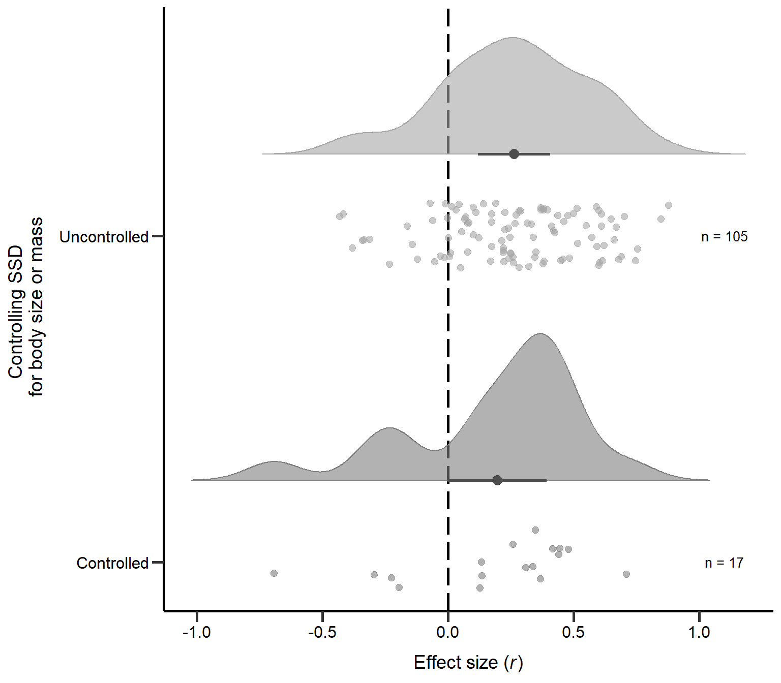
Figure S2B: Raincloud plot of correlation coefficients for primary studies controlling SSD for body size or mass (uncontrolled or controlled) including sample sizes and estimates with 95% CI from phylogenetic model.
Phylogentic vs non-phylogenetic studies
Next we explored the effect of studies controlling for phylogeny vs non-phylogenetic studies:
MetaData$PhyloControlled=as.factor(MetaData$PhyloControlled)
MetaData$PhyloControlled=relevel(MetaData$PhyloControlled,c("No"))
Model_cREML_by_Phylo = rma.mv(r ~ PhyloControlled, V=Var_r, data = MetaData, random = c(~ 1 | Study_ID,~ 1 | Index, ~ 1 | Class), R = list(Class = forcedC_Moderators), method = "REML")
summary(Model_cREML_by_Phylo)
Multivariate Meta-Analysis Model (k = 122; method: REML)

  logLik  Deviance       AIC       BIC      AICc
-20.7468   41.4937   51.4937   65.4311   52.0200

Variance Components:

            estim    sqrt  nlvls  fixed    factor    R
sigma^2.1  0.0134  0.1159     73     no  Study_ID   no
sigma^2.2  0.0503  0.2244    122     no     Index   no
sigma^2.3  0.0117  0.1083     11     no     Class  yes

Test for Residual Heterogeneity:
QE(df = 120) = 1350.6816, p-val < .0001

Test of Moderators (coefficient 2):
QM(df = 1) = 6.8605, p-val = 0.0088

Model Results:

                    estimate      se     zval    pval    ci.lb    ci.ub
intrcpt               0.4194  0.0959   4.3714  <.0001   0.2314   0.6075  ***
PhyloControlledYes   -0.2067  0.0789  -2.6192  0.0088  -0.3614  -0.0520   **

---
Signif. codes:  0 '***' 0.001 '**' 0.01 '*' 0.05 '.' 0.1 ' ' 1
We then re-leveled the model for post-hoc comparisons:
MetaData$PhyloControlled=relevel(MetaData$PhyloControlled,c("Yes"))
Model_cREML_by_Phylo2 = rma.mv(r ~ PhyloControlled, V=Var_r, data = MetaData, random = c(~ 1 | Study_ID,~ 1 | Index, ~ 1 | Class), R = list(Class = forcedC_Moderators), method = "REML")
summary(Model_cREML_by_Phylo2)
Finally, we computed FDR corrected p-values:
tab5=as.data.frame(round(p.adjust(c(0.0001, 0.0027), method = 'fdr'),digit=3),row.names=cbind("Non-phylogenetic","With phylogeny"))
colnames(tab5)<-cbind('P-value')
tab5
P-value
Non-phylogenetic 0.000
With phylogeny 0.003Plot Phylogentic vs non-phylogenetic studies (Figure S2C)
Here we plot the type of SSD measure moderator:
MetaData$PhyloControlled=as.factor(MetaData$PhyloControlled)
MetaData$PhyloControlled=relevel(MetaData$PhyloControlled,c("No"))

ggplot(MetaData, aes(x=PhyloControlled, y=r, fill = PhyloControlled, colour = PhyloControlled)) +
  geom_hline(yintercept=0, linetype="longdash", color = "black", linewidth=1)+
  geom_flat_violin(position = position_nudge(x = 0.25, y = 0),adjust =1, trim = F,alpha=0.6)+
  geom_point(position = position_jitter(width = .1), size = 2.5,alpha=0.6,stroke=0,shape=19)+
  geom_point(inherit.aes = F,mapping = aes(y=Model_cREML_by_Phylo2$b[1,1], x=2.25), size = 3.5,alpha=1,stroke=0,shape=19,color='grey30')+
  geom_point(inherit.aes = F,mapping = aes(y=Model_cREML_by_Phylo$b[1,1], x=1.25), size = 3.5,alpha=1,stroke=0,shape=19,color='grey30')+
  geom_segment(inherit.aes = F,mapping = aes(y=Model_cREML_by_Phylo2$ci.lb[1], x=2.25, xend= 2.25, yend= Model_cREML_by_Phylo2$ci.ub[1]), alpha=1,linewidth=1,color='grey30')+
  geom_segment(inherit.aes = F,mapping = aes(y=Model_cREML_by_Phylo$ci.lb[1], x=1.25, xend= 1.25, yend= Model_cREML_by_Phylo$ci.ub[1]), alpha=1,linewidth=1,color='grey30')+
  ylab(expression(paste("Effect size (", italic("r"),')')))+xlab('Controlling for phylogeny')+coord_flip()+guides(fill = FALSE, colour = FALSE) +
  scale_color_manual(values =colpal4)+
  scale_fill_manual(values =colpal4)+
  scale_x_discrete(labels=(c("Phylogenetically \n uncorrected ","Phylogenetically \n corrected ")),expand=c(.15,0))+
  annotate("text", x=1, y=1.1, label= "n = 20",size=3.5) +
  annotate("text", x=2, y=1.1, label= "n = 102",size=3.5)  + theme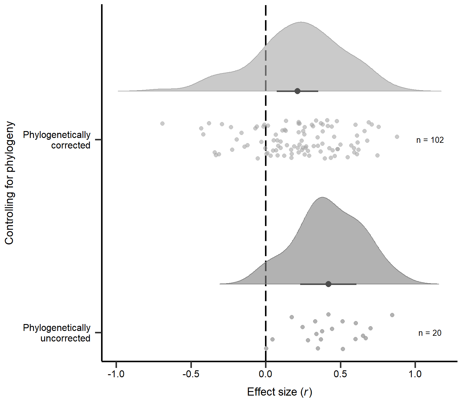
Figure S2C: Raincloud plot of correlation coefficients for non-phylogenetic and phylogenetic analyses in primary studies including sample sizes and estimates with 95% CI from phylogenetic model (Table 4).
Percentage of species with female-biased SSD
There was variation in the primary studies regarding the typical SSD in the studied taxa (i.e. some studies focused on taxa with more male-biased SSD, while others on taxa with more female-biased SSD). Still, there was no significant relationship between the percentage of species with a female-biased SSD and effect sizes.
MetaData_SSDbias=MetaData
MetaData_SSDbias=MetaData_SSDbias[!is.na(MetaData_SSDbias$SSD_SexBias_in_perc_F),]
Model_REML_SSbias         = rma.mv(r ~ SSD_SexBias_in_perc_F, V=Var_r, data = MetaData_SSDbias, random = c(~ 1 | Study_ID,~ 1 | Index, ~ 1 | Class), R = list(Class = forcedC_Moderators), method = "REML")
summary(Model_REML_SSbias)
Multivariate Meta-Analysis Model (k = 104; method: REML)

  logLik  Deviance       AIC       BIC      AICc
-20.8873   41.7746   51.7746   64.8995   52.3996

Variance Components:

            estim    sqrt  nlvls  fixed    factor    R
sigma^2.1  0.0280  0.1673     64     no  Study_ID   no
sigma^2.2  0.0471  0.2170    104     no     Index   no
sigma^2.3  0.0051  0.0716     11     no     Class  yes

Test for Residual Heterogeneity:
QE(df = 102) = 1443.6764, p-val < .0001

Test of Moderators (coefficient 2):
QM(df = 1) = 3.2778, p-val = 0.0702

Model Results:

                       estimate      se     zval    pval    ci.lb   ci.ub
intrcpt                  0.3765  0.0807   4.6657  <.0001   0.2183  0.5346  ***
SSD_SexBias_in_perc_F   -0.0021  0.0012  -1.8105  0.0702  -0.0044  0.0002    .

---
Signif. codes:  0 '***' 0.001 '**' 0.01 '*' 0.05 '.' 0.1 ' ' 1
Figure S3A
model_p1 <- predict(Model_REML_SSbias) # Extract model predictions

ggplot(MetaData_SSDbias, aes(x=as.numeric(SSD_SexBias_in_perc_F), y=r)) +
  theme(panel.grid.major = element_blank(), panel.grid.minor = element_blank(),panel.background = element_blank(), axis.line = element_line(colour = "black"))+
  theme(axis.text=element_text(size=13),
        axis.title=element_text(size=14))+ theme(legend.position="none")+
  geom_point(shape=16, size = 3,alpha=0.5)+xlab('% of species with \n female-biased SSD')+ylab(expression(paste("Effect size (", italic("r"),')')))+
  geom_hline(yintercept=0, linetype="dashed", color = "black", linewidth=1)+
  geom_line( aes(y = model_p1$pred), size = 1)+
  geom_ribbon( aes(ymin = model_p1$ci.lb, ymax = model_p1$ci.ub, color = 'black',linetype=NA), alpha = .15,show.legend = F, outline.type = "both") +
  theme
Figure S3A: Scatter plot of the sPercentage of species with a female-biased SSD. Dashed line marks a correlation coefficient of zero, black line represents predictions from REML model (controlling for phylogeny) and grey area represents 95% CI on model predictions.
Test for publication bias
To test for publication bias, we transformed r into z scores and ran multilevel mixed-effects models (restricted maximum likelihood) with z as the predictor and its standard error as the response with study ID and an observation level random effect. Models were weight by the mean standard error of z across all studies. While the variance in r depends on the effect size and the sample size, the variance in z is only dependent on the sample size. Hence, if z values correlate with the variance in z, this indicates that small studies were only published, if the effect was large, suggesting publication bias.
Model_REML_PublBias         = rma.mv(z ~ SE_z, V=rep((mean(SE_z)*mean(SE_z))*N,length(SE_z)), data = MetaData, random = c(~ 1 | Study_ID,~ 1 | Index, ~ 1 | Class), R = list(Class = forcedC_Moderators), method = "REML",control=list(rel.tol=1e-8))
summary(Model_REML_PublBias)
Multivariate Meta-Analysis Model (k = 122; method: REML)

   logLik   Deviance        AIC        BIC       AICc
-145.5101   291.0202   301.0202   314.9577   301.5465

Variance Components:

            estim    sqrt  nlvls  fixed    factor    R
sigma^2.1  0.0000  0.0000     73     no  Study_ID   no
sigma^2.2  0.0000  0.0000    122     no     Index   no
sigma^2.3  0.0000  0.0002     11     no     Class  yes

Test for Residual Heterogeneity:
QE(df = 120) = 19.2579, p-val = 1.0000

Test of Moderators (coefficient 2):
QM(df = 1) = 1.5648, p-val = 0.2110

Model Results:

         estimate      se    zval    pval    ci.lb   ci.ub
intrcpt    0.1715  0.1977  0.8678  0.3855  -0.2159  0.5590
SE_z       0.8181  0.6540  1.2509  0.2110  -0.4637  2.0999

---
Signif. codes:  0 '***' 0.001 '**' 0.01 '*' 0.05 '.' 0.1 ' ' 1
Figure S3B
# Extract model predictions
model_p2 <- predict(Model_REML_PublBias)

ggplot(MetaData, aes(x=SE_z, y=z)) +
  theme(panel.grid.major = element_blank(), panel.grid.minor = element_blank(),panel.background = element_blank(), axis.line = element_line(colour = "black"))+
  theme(axis.text=element_text(size=13),
        axis.title=element_text(size=14))+ theme(legend.position="none")+ylab(expression(paste("Effect size (", italic("z"),')')))+
  geom_point(shape=16, size = 3,alpha=0.5)+xlab('Standard error')+
  geom_hline(yintercept=0, linetype="dashed", color = "black", linewidth=1)+
  geom_line( aes(y = model_p2$pred), size = 1)+
  geom_ribbon( aes(ymin = model_p2$ci.lb, ymax = model_p2$ci.ub, color = 'black',linetype=NA), alpha = .15,show.legend = F, outline.type = "both") +
  theme
Figure S3B: Scatter plot of the standard error in z scores of each study against the z score of each primary study (transformed correlation coefficients). Dashed line marks a correlation coefficient of zero, black line represents predictions from REML model (controlling for phylogeny) and grey area represents 95% CI on model predictions.
Publication year
Next we explored the effect of the publication year of each study:
Model_REML_by_Year = rma.mv(r ~ Year, V=Var_r, data = MetaData, random = c(~ 1 | Study_ID,~ 1 | Index, ~ 1 | Class), R = list(Class = forcedC_Moderators), method = "REML")
summary(Model_REML_by_Year)
Multivariate Meta-Analysis Model (k = 122; method: REML)

  logLik  Deviance       AIC       BIC      AICc
-21.5680   43.1360   53.1360   67.0735   53.6623

Variance Components:

            estim    sqrt  nlvls  fixed    factor    R
sigma^2.1  0.0177  0.1332     73     no  Study_ID   no
sigma^2.2  0.0476  0.2183    122     no     Index   no
sigma^2.3  0.0118  0.1085     11     no     Class  yes

Test for Residual Heterogeneity:
QE(df = 120) = 1275.7703, p-val < .0001

Test of Moderators (coefficient 2):
QM(df = 1) = 5.0277, p-val = 0.0249

Model Results:

         estimate      se     zval    pval    ci.lb    ci.ub
intrcpt   11.7151  5.1141   2.2907  0.0220   1.6917  21.7385  *
Year      -0.0057  0.0025  -2.2423  0.0249  -0.0107  -0.0007  *

---
Signif. codes:  0 '***' 0.001 '**' 0.01 '*' 0.05 '.' 0.1 ' ' 1
Plot publication year (Figure S3C)
Here we plot the publication year:
# Extract model predictions
Model_REML_by_Year = rma.mv(r ~ Year, V=Var_r, data = MetaData, random = c(~ 1 | Study_ID,~ 1 | Index, ~ 1 | Class), R = list(Class = forcedC_Moderators), method = "REML")
model_p4 <- predict(Model_REML_by_Year)

ggplot(MetaData, aes(x=as.numeric(Year), y=r)) +
  theme(panel.grid.major = element_blank(), panel.grid.minor = element_blank(),panel.background = element_blank(), axis.line = element_line(colour = "black"))+
  theme(axis.text=element_text(size=13),
        axis.title=element_text(size=14))+ theme(legend.position="none")+
  geom_point(shape=16, size = 3,alpha=0.5)+xlab('Publication year')+ylab(expression(paste("Effect size (", italic("r"),')')))+
  geom_hline(yintercept=0, linetype="dashed", color = "black", linewidth=1)+
  geom_line( aes(y = model_p4$pred), size = 1)+
  geom_ribbon( aes(ymin = model_p4$ci.lb, ymax = model_p4$ci.ub, color = 'black',linetype=NA), alpha = .15,show.legend = F, outline.type = "both") +
  theme
Figure S3C: Scatter plot of correlation coefficients against the publication year of each study. Dashed line marks a correlation coefficient of zero, black line represents predictions from REML model (controlling for phylogeny) and grey area represents 95% CI on model predictions.
Moderator tests for non-phylogenetic models
Here we ran all models without the phylogeny.
Sexual selection episode
The first model explores the effect of the sexual selection episode (i.e. pre-copulatory, post-copulatory or both):
MetaData$SexSel_Episode=relevel(MetaData$SexSel_Episode,c("pre-copulatory"))
Model_REML_by_cSexSelEpisode = rma.mv(r ~ factor(SexSel_Episode), V=Var_r, data = MetaData, random = c(~ 1 | Study_ID,~ 1 | Index), method = "REML")
summary(Model_REML_by_cSexSelEpisode)
Multivariate Meta-Analysis Model (k = 122; method: REML)

  logLik  Deviance       AIC       BIC      AICc
-10.3162   20.6324   30.6324   44.5280   31.1634

Variance Components:

            estim    sqrt  nlvls  fixed    factor
sigma^2.1  0.0243  0.1559     73     no  Study_ID
sigma^2.2  0.0337  0.1836    122     no     Index

Test for Residual Heterogeneity:
QE(df = 119) = 1337.5244, p-val < .0001

Test of Moderators (coefficients 2:3):
QM(df = 2) = 34.5137, p-val < .0001

Model Results:

                                       estimate      se     zval    pval
intrcpt                                  0.2379  0.0407   5.8383  <.0001
factor(SexSel_Episode)both               0.1673  0.0543   3.0825  0.0021
factor(SexSel_Episode)post-copulatory   -0.3150  0.0833  -3.7828  0.0002
                                         ci.lb    ci.ub
intrcpt                                 0.1580   0.3177  ***
factor(SexSel_Episode)both              0.0609   0.2737   **
factor(SexSel_Episode)post-copulatory  -0.4783  -0.1518  ***

---
Signif. codes:  0 '***' 0.001 '**' 0.01 '*' 0.05 '.' 0.1 ' ' 1
We then re-leveled the model for post-hoc comparisons:
MetaData$SexSel_Episode=relevel(MetaData$SexSel_Episode,c("post-copulatory"))
Model_REML_by_cSexSelEpisode2 = rma.mv(r ~ factor(SexSel_Episode), V=Var_r, data = MetaData, random = c(~ 1 | Study_ID,~ 1 | Index), method = "REML")
summary(Model_REML_by_cSexSelEpisode2)

MetaData$SexSel_Episode=relevel(MetaData$SexSel_Episode,c("both"))
Model_REML_by_cSexSelEpisode3 = rma.mv(r ~ factor(SexSel_Episode), V=Var_r, data = MetaData, random = c(~ 1 | Study_ID,~ 1 | Index),  method = "REML")
summary(Model_REML_by_cSexSelEpisode3)
Finally, we computed FDR corrected p-values:
tab1=as.data.frame(round(p.adjust(c(0.0001, 0.2970, .0001), method = 'fdr'),digit=3),row.names=cbind("Pre-copulatory","Post-copulatory","Both"))
colnames(tab1)<-cbind('P-value')
tab1
P-value
Pre-copulatory 0.000
Post-copulatory 0.297
Both 0.000Sexual selection category
Next we explored the effect of the sexual selection category (i.e. density, mating system, operational sex ratio (OSR), post-mating competition, pre-mating competition, trait-based, other):
MetaData$SexSel_Category=as.factor(MetaData$SexSel_Category)
MetaData$SexSel_Category=relevel(MetaData$SexSel_Category,c("Postmating competition"))
Model_REML_by_cSexSelCat = rma.mv(r ~ factor(SexSel_Category), V=Var_r, data = MetaData, random = c(~ 1 | Study_ID,~ 1 | Index), method = "REML")
summary(Model_REML_by_cSexSelCat)
Multivariate Meta-Analysis Model (k = 122; method: REML)

  logLik  Deviance       AIC       BIC      AICc
  4.7833   -9.5666    8.4334   33.1378   10.1477

Variance Components:

            estim    sqrt  nlvls  fixed    factor
sigma^2.1  0.0268  0.1636     73     no  Study_ID
sigma^2.2  0.0181  0.1346    122     no     Index

Test for Residual Heterogeneity:
QE(df = 115) = 916.8832, p-val < .0001

Test of Moderators (coefficients 2:7):
QM(df = 6) = 83.7704, p-val < .0001

Model Results:

                                              estimate      se     zval    pval
intrcpt                                        -0.0721  0.0685  -1.0516  0.2930
factor(SexSel_Category)Other                    0.4433  0.0942   4.7044  <.0001
factor(SexSel_Category)OSR                      0.7141  0.1285   5.5581  <.0001
factor(SexSel_Category)Mating system            0.4713  0.0792   5.9503  <.0001
factor(SexSel_Category)Premating competition    0.4308  0.0837   5.1490  <.0001
factor(SexSel_Category)Density                  0.3274  0.1226   2.6695  0.0076
factor(SexSel_Category)Trait-based              0.0776  0.0880   0.8815  0.3780
                                                ci.lb   ci.ub
intrcpt                                       -0.2064  0.0622
factor(SexSel_Category)Other                   0.2586  0.6280  ***
factor(SexSel_Category)OSR                     0.4623  0.9659  ***
factor(SexSel_Category)Mating system           0.3161  0.6266  ***
factor(SexSel_Category)Premating competition   0.2668  0.5948  ***
factor(SexSel_Category)Density                 0.0870  0.5678   **
factor(SexSel_Category)Trait-based            -0.0949  0.2500

---
Signif. codes:  0 '***' 0.001 '**' 0.01 '*' 0.05 '.' 0.1 ' ' 1
We then re-leveled the model for post-hoc comparisons:
MetaData$SexSel_Category=relevel(MetaData$SexSel_Category,c("Trait-based"))
Model_REML_by_cSexSelCat2 = rma.mv(r ~ factor(SexSel_Category), V=Var_r, data = MetaData, random = c(~ 1 | Study_ID,~ 1 | Index), method = "REML")
summary(Model_REML_by_cSexSelCat2)

MetaData$SexSel_Category=relevel(MetaData$SexSel_Category,c("Density"))
Model_REML_by_cSexSelCat3 = rma.mv(r ~ factor(SexSel_Category), V=Var_r, data = MetaData, random = c(~ 1 | Study_ID,~ 1 | Index), method = "REML")
summary(Model_REML_by_cSexSelCat3)

MetaData$SexSel_Category=relevel(MetaData$SexSel_Category,c("Premating competition"))
Model_REML_by_cSexSelCat4 = rma.mv(r ~ factor(SexSel_Category), V=Var_r, data = MetaData, random = c(~ 1 | Study_ID,~ 1 | Index), method = "REML")
summary(Model_REML_by_cSexSelCat4)

MetaData$SexSel_Category=relevel(MetaData$SexSel_Category,c("Mating system"))
Model_REML_by_cSexSelCat5 = rma.mv(r ~ factor(SexSel_Category), V=Var_r, data = MetaData, random = c(~ 1 | Study_ID,~ 1 | Index), method = "REML")
summary(Model_REML_by_cSexSelCat5)

MetaData$SexSel_Category=relevel(MetaData$SexSel_Category,c("OSR"))
Model_REML_by_cSexSelCat6 = rma.mv(r ~ factor(SexSel_Category), V=Var_r, data = MetaData, random = c(~ 1 | Study_ID,~ 1 | Index), method = "REML")
summary(Model_REML_by_cSexSelCat6)

MetaData$SexSel_Category=relevel(MetaData$SexSel_Category,c("Other"))
Model_REML_by_cSexSelCat7 = rma.mv(r ~ factor(SexSel_Category), V=Var_r, data = MetaData, random = c(~ 1 | Study_ID,~ 1 | Index), method = "REML")
summary(Model_REML_by_cSexSelCat7)
Finally, we computed FDR corrected p-values:
tab2=as.data.frame(round(p.adjust(c(0.2930, 0.9215, 0.0124, .0001, .0001, .0001, .0001), method = 'fdr'),digit=3),row.names=cbind("Postmating competition","Trait-based","Density",'Premating competition',"Mating system","OSR","Other"))
colnames(tab2)<-cbind('P-value')
tab2
P-value
Postmating competition 0.342
Trait-based 0.921
Density 0.017
Premating competition 0.000
Mating system 0.000
OSR 0.000
Other 0.000Phylogenetic classes
Next we explored the effect of the phylogenetic classes:
MetaData$Class=relevel(MetaData$Class,c("Actinopterygii"))
Model_cREML_by_Class5 = rma.mv(r ~ Class, V=Var_r, data = MetaData, random = c(~ 1 | Study_ID,~ 1 | Index), method = "REML")
summary(Model_cREML_by_Class5)
Multivariate Meta-Analysis Model (k = 122; method: REML)

  logLik  Deviance       AIC       BIC      AICc
-19.8965   39.7930   65.7930  101.0169   69.5455

Variance Components:

            estim    sqrt  nlvls  fixed    factor
sigma^2.1  0.0183  0.1352     73     no  Study_ID
sigma^2.2  0.0512  0.2262    122     no     Index

Test for Residual Heterogeneity:
QE(df = 111) = 1222.6024, p-val < .0001

Test of Moderators (coefficients 2:11):
QM(df = 10) = 16.3649, p-val = 0.0897

Model Results:

                   estimate      se     zval    pval    ci.lb   ci.ub
intrcpt              0.2199  0.1099   2.0012  0.0454   0.0045  0.4352  *
ClassAmphibia       -0.1432  0.1483  -0.9659  0.3341  -0.4338  0.1474
ClassAnimalia        0.0060  0.2469   0.0244  0.9805  -0.4780  0.4900
ClassAves           -0.0023  0.1223  -0.0187  0.9851  -0.2419  0.2373
ClassInsecta         0.1621  0.1586   1.0222  0.3067  -0.1487  0.4729
ClassMalacostraca   -0.2177  0.3535  -0.6157  0.5381  -0.9106  0.4753
ClassMammalia        0.1666  0.1195   1.3939  0.1633  -0.0677  0.4009
ClassNematoda        0.2021  0.2646   0.7637  0.4450  -0.3165  0.7208
ClassPisces          0.0384  0.2897   0.1327  0.8944  -0.5293  0.6062
ClassReptilia       -0.0980  0.1426  -0.6870  0.4921  -0.3775  0.1816
ClassTrematoda      -0.1598  0.2298  -0.6954  0.4868  -0.6102  0.2906

---
Signif. codes: 0 '***' 0.001 '**' 0.01 '*' 0.05 '.' 0.1 ' ' 1MetaData$Class=relevel(MetaData$Class,c("Amphibia"))
Model_cREML_by_Class4 = rma.mv(r ~ Class, V=Var_r, data = MetaData, random = c(~ 1 | Study_ID,~ 1 | Index), method = "REML")
summary(Model_cREML_by_Class4)
Multivariate Meta-Analysis Model (k = 122; method: REML)

  logLik  Deviance       AIC       BIC      AICc
-19.8965   39.7930   65.7930  101.0169   69.5455

Variance Components:

            estim    sqrt  nlvls  fixed    factor
sigma^2.1  0.0183  0.1352     73     no  Study_ID
sigma^2.2  0.0512  0.2262    122     no     Index

Test for Residual Heterogeneity:
QE(df = 111) = 1222.6024, p-val < .0001

Test of Moderators (coefficients 2:11):
QM(df = 10) = 16.3649, p-val = 0.0897

Model Results:

                     estimate      se     zval    pval    ci.lb   ci.ub
intrcpt                0.0766  0.0996   0.7697  0.4415  -0.1185  0.2718
ClassActinopterygii    0.1432  0.1483   0.9659  0.3341  -0.1474  0.4338
ClassAnimalia          0.1492  0.2425   0.6153  0.5383  -0.3261  0.6246
ClassAves              0.1409  0.1137   1.2394  0.2152  -0.0819  0.3638
ClassInsecta           0.3053  0.1524   2.0028  0.0452   0.0065  0.6041   *
ClassMalacostraca     -0.0744  0.3505  -0.2124  0.8318  -0.7614  0.6125
ClassMammalia          0.3098  0.1112   2.7860  0.0053   0.0919  0.5278  **
ClassNematoda          0.3453  0.2605   1.3255  0.1850  -0.1653  0.8559
ClassPisces            0.1817  0.2859   0.6353  0.5252  -0.3788  0.7421
ClassReptilia          0.0452  0.1349   0.3353  0.7374  -0.2192  0.3096
ClassTrematoda        -0.0166  0.2291  -0.0724  0.9423  -0.4656  0.4324

---
Signif. codes: 0 '***' 0.001 '**' 0.01 '*' 0.05 '.' 0.1 ' ' 1MetaData$Class=relevel(MetaData$Class,c("Animalia"))
Model_cREML_by_Class11 = rma.mv(r ~ Class, V=Var_r, data = MetaData, random = c(~ 1 | Study_ID,~ 1 | Index), method = "REML")
summary(Model_cREML_by_Class11)
Multivariate Meta-Analysis Model (k = 122; method: REML)

  logLik  Deviance       AIC       BIC      AICc
-19.8965   39.7930   65.7930  101.0169   69.5455

Variance Components:

            estim    sqrt  nlvls  fixed    factor
sigma^2.1  0.0183  0.1352     73     no  Study_ID
sigma^2.2  0.0512  0.2262    122     no     Index

Test for Residual Heterogeneity:
QE(df = 111) = 1222.6024, p-val < .0001

Test of Moderators (coefficients 2:11):
QM(df = 10) = 16.3649, p-val = 0.0897

Model Results:

                     estimate      se     zval    pval    ci.lb   ci.ub
intrcpt                0.2259  0.2212   1.0214  0.3071  -0.2076  0.6594
ClassAmphibia         -0.1492  0.2425  -0.6153  0.5383  -0.6246  0.3261
ClassActinopterygii   -0.0060  0.2469  -0.0244  0.9805  -0.4900  0.4780
ClassAves             -0.0083  0.2279  -0.0365  0.9709  -0.4549  0.4383
ClassInsecta           0.1561  0.2495   0.6256  0.5316  -0.3329  0.6450
ClassMalacostraca     -0.2237  0.4023  -0.5560  0.5782  -1.0121  0.5648
ClassMammalia          0.1606  0.2266   0.7085  0.4786  -0.2836  0.6048
ClassNematoda          0.1961  0.3269   0.5998  0.5486  -0.4446  0.8368
ClassPisces            0.0324  0.3475   0.0933  0.9257  -0.6487  0.7135
ClassReptilia         -0.1040  0.2392  -0.4349  0.6636  -0.5728  0.3647
ClassTrematoda        -0.1658  0.3025  -0.5483  0.5835  -0.7586  0.4270

---
Signif. codes: 0 '***' 0.001 '**' 0.01 '*' 0.05 '.' 0.1 ' ' 1MetaData$Class=relevel(MetaData$Class,c("Aves"))
Model_cREML_by_Class = rma.mv(r ~ Class, V=Var_r, data = MetaData, random = c(~ 1 | Study_ID,~ 1 | Index), method = "REML")
summary(Model_cREML_by_Class)
Multivariate Meta-Analysis Model (k = 122; method: REML)

  logLik  Deviance       AIC       BIC      AICc
-19.8965   39.7930   65.7930  101.0169   69.5455

Variance Components:

            estim    sqrt  nlvls  fixed    factor
sigma^2.1  0.0183  0.1352     73     no  Study_ID
sigma^2.2  0.0512  0.2262    122     no     Index

Test for Residual Heterogeneity:
QE(df = 111) = 1222.6024, p-val < .0001

Test of Moderators (coefficients 2:11):
QM(df = 10) = 16.3649, p-val = 0.0897

Model Results:

                     estimate      se     zval    pval    ci.lb   ci.ub
intrcpt                0.2176  0.0549   3.9626  <.0001   0.1100  0.3252  ***
ClassAnimalia          0.0083  0.2279   0.0365  0.9709  -0.4383  0.4549
ClassAmphibia         -0.1409  0.1137  -1.2394  0.2152  -0.3638  0.0819
ClassActinopterygii    0.0023  0.1223   0.0187  0.9851  -0.2373  0.2419
ClassInsecta           0.1644  0.1276   1.2880  0.1977  -0.0858  0.4145
ClassMalacostraca     -0.2154  0.3405  -0.6325  0.5270  -0.8827  0.4520
ClassMammalia          0.1689  0.0731   2.3113  0.0208   0.0257  0.3121    *
ClassNematoda          0.2044  0.2469   0.8277  0.4078  -0.2796  0.6883
ClassPisces            0.0407  0.2736   0.1489  0.8817  -0.4955  0.5770
ClassReptilia         -0.0957  0.1056  -0.9064  0.3647  -0.3026  0.1112
ClassTrematoda        -0.1575  0.2126  -0.7409  0.4588  -0.5742  0.2592

---
Signif. codes: 0 '***' 0.001 '**' 0.01 '*' 0.05 '.' 0.1 ' ' 1MetaData$Class=relevel(MetaData$Class,c("Insecta"))
Model_cREML_by_Class8 = rma.mv(r ~ Class, V=Var_r, data = MetaData, random = c(~ 1 | Study_ID,~ 1 | Index), method = "REML")
summary(Model_cREML_by_Class8)
Multivariate Meta-Analysis Model (k = 122; method: REML)

  logLik  Deviance       AIC       BIC      AICc
-19.8965   39.7930   65.7930  101.0169   69.5455

Variance Components:

            estim    sqrt  nlvls  fixed    factor
sigma^2.1  0.0183  0.1352     73     no  Study_ID
sigma^2.2  0.0512  0.2262    122     no     Index

Test for Residual Heterogeneity:
QE(df = 111) = 1222.6024, p-val < .0001

Test of Moderators (coefficients 2:11):
QM(df = 10) = 16.3649, p-val = 0.0897

Model Results:

                     estimate      se     zval    pval    ci.lb    ci.ub
intrcpt                0.3819  0.1154   3.3090  0.0009   0.1557   0.6082  ***
ClassAves             -0.1644  0.1276  -1.2880  0.1977  -0.4145   0.0858
ClassAnimalia         -0.1561  0.2495  -0.6256  0.5316  -0.6450   0.3329
ClassAmphibia         -0.3053  0.1524  -2.0028  0.0452  -0.6041  -0.0065    *
ClassActinopterygii   -0.1621  0.1586  -1.0222  0.3067  -0.4729   0.1487
ClassMalacostraca     -0.3797  0.3553  -1.0688  0.2852  -1.0761   0.3166
ClassMammalia          0.0045  0.1252   0.0361  0.9712  -0.2409   0.2500
ClassNematoda          0.0400  0.2670   0.1499  0.8808  -0.4833   0.5633
ClassPisces           -0.1236  0.2918  -0.4237  0.6718  -0.6956   0.4484
ClassReptilia         -0.2601  0.1470  -1.7694  0.0768  -0.5481   0.0280    .
ClassTrematoda        -0.3219  0.2349  -1.3702  0.1706  -0.7823   0.1386

---
Signif. codes: 0 '***' 0.001 '**' 0.01 '*' 0.05 '.' 0.1 ' ' 1MetaData$Class=relevel(MetaData$Class,c("Malacostraca"))
Model_cREML_by_Class7 = rma.mv(r ~ Class, V=Var_r, data = MetaData, random = c(~ 1 | Study_ID,~ 1 | Index), method = "REML")
summary(Model_cREML_by_Class7)
Multivariate Meta-Analysis Model (k = 122; method: REML)

  logLik  Deviance       AIC       BIC      AICc
-19.8965   39.7930   65.7930  101.0169   69.5455

Variance Components:

            estim    sqrt  nlvls  fixed    factor
sigma^2.1  0.0183  0.1352     73     no  Study_ID
sigma^2.2  0.0512  0.2262    122     no     Index

Test for Residual Heterogeneity:
QE(df = 111) = 1222.6024, p-val < .0001

Test of Moderators (coefficients 2:11):
QM(df = 10) = 16.3649, p-val = 0.0897

Model Results:

                     estimate      se    zval    pval    ci.lb   ci.ub
intrcpt                0.0022  0.3360  0.0065  0.9948  -0.6564  0.6608
ClassInsecta           0.3797  0.3553  1.0688  0.2852  -0.3166  1.0761
ClassAves              0.2154  0.3405  0.6325  0.5270  -0.4520  0.8827
ClassAnimalia          0.2237  0.4023  0.5560  0.5782  -0.5648  1.0121
ClassAmphibia          0.0744  0.3505  0.2124  0.8318  -0.6125  0.7614
ClassActinopterygii    0.2177  0.3535  0.6157  0.5381  -0.4753  0.9106
ClassMammalia          0.3843  0.3397  1.1313  0.2579  -0.2815  1.0500
ClassNematoda          0.4198  0.4134  1.0155  0.3099  -0.3904  1.2300
ClassPisces            0.2561  0.4298  0.5958  0.5513  -0.5864  1.0986
ClassReptilia          0.1197  0.3481  0.3437  0.7310  -0.5627  0.8020
ClassTrematoda         0.0578  0.3943  0.1467  0.8834  -0.7150  0.8307

---
Signif. codes: 0 '***' 0.001 '**' 0.01 '*' 0.05 '.' 0.1 ' ' 1MetaData$Class=relevel(MetaData$Class,c("Mammalia"))
Model_cREML_by_Class3 = rma.mv(r ~ Class, V=Var_r, data = MetaData, random = c(~ 1 | Study_ID,~ 1 | Index), method = "REML")
summary(Model_cREML_by_Class3)
Multivariate Meta-Analysis Model (k = 122; method: REML)

  logLik  Deviance       AIC       BIC      AICc
-19.8965   39.7930   65.7930  101.0169   69.5455

Variance Components:

            estim    sqrt  nlvls  fixed    factor
sigma^2.1  0.0183  0.1352     73     no  Study_ID
sigma^2.2  0.0512  0.2262    122     no     Index

Test for Residual Heterogeneity:
QE(df = 111) = 1222.6024, p-val < .0001

Test of Moderators (coefficients 2:11):
QM(df = 10) = 16.3649, p-val = 0.0897

Model Results:

                     estimate      se     zval    pval    ci.lb    ci.ub
intrcpt                0.3865  0.0495   7.8052  <.0001   0.2894   0.4835  ***
ClassMalacostraca     -0.3843  0.3397  -1.1313  0.2579  -1.0500   0.2815
ClassInsecta          -0.0045  0.1252  -0.0361  0.9712  -0.2500   0.2409
ClassAves             -0.1689  0.0731  -2.3113  0.0208  -0.3121  -0.0257    *
ClassAnimalia         -0.1606  0.2266  -0.7085  0.4786  -0.6048   0.2836
ClassAmphibia         -0.3098  0.1112  -2.7860  0.0053  -0.5278  -0.0919   **
ClassActinopterygii   -0.1666  0.1195  -1.3939  0.1633  -0.4009   0.0677
ClassNematoda          0.0355  0.2458   0.1444  0.8851  -0.4462   0.5172
ClassPisces           -0.1282  0.2726  -0.4702  0.6382  -0.6624   0.4061
ClassReptilia         -0.2646  0.1031  -2.5675  0.0102  -0.4666  -0.0626    *
ClassTrematoda        -0.3264  0.2106  -1.5498  0.1212  -0.7392   0.0864

---
Signif. codes: 0 '***' 0.001 '**' 0.01 '*' 0.05 '.' 0.1 ' ' 1MetaData$Class=relevel(MetaData$Class,c("Nematoda"))
Model_cREML_by_Class10 = rma.mv(r ~ Class, V=Var_r, data = MetaData, random = c(~ 1 | Study_ID,~ 1 | Index), method = "REML")
summary(Model_cREML_by_Class10)
Multivariate Meta-Analysis Model (k = 122; method: REML)

  logLik  Deviance       AIC       BIC      AICc
-19.8965   39.7930   65.7930  101.0169   69.5455

Variance Components:

            estim    sqrt  nlvls  fixed    factor
sigma^2.1  0.0183  0.1352     73     no  Study_ID
sigma^2.2  0.0512  0.2262    122     no     Index

Test for Residual Heterogeneity:
QE(df = 111) = 1222.6024, p-val < .0001

Test of Moderators (coefficients 2:11):
QM(df = 10) = 16.3649, p-val = 0.0897

Model Results:

                     estimate      se     zval    pval    ci.lb   ci.ub
intrcpt                0.4220  0.2407   1.7528  0.0796  -0.0499  0.8938  .
ClassMammalia         -0.0355  0.2458  -0.1444  0.8851  -0.5172  0.4462
ClassMalacostraca     -0.4198  0.4134  -1.0155  0.3099  -1.2300  0.3904
ClassInsecta          -0.0400  0.2670  -0.1499  0.8808  -0.5633  0.4833
ClassAves             -0.2044  0.2469  -0.8277  0.4078  -0.6883  0.2796
ClassAnimalia         -0.1961  0.3269  -0.5998  0.5486  -0.8368  0.4446
ClassAmphibia         -0.3453  0.2605  -1.3255  0.1850  -0.8559  0.1653
ClassActinopterygii   -0.2021  0.2646  -0.7637  0.4450  -0.7208  0.3165
ClassPisces           -0.1637  0.3603  -0.4543  0.6496  -0.8698  0.5425
ClassReptilia         -0.3001  0.2574  -1.1660  0.2436  -0.8045  0.2044
ClassTrematoda        -0.3619  0.3171  -1.1415  0.2537  -0.9833  0.2595

---
Signif. codes: 0 '***' 0.001 '**' 0.01 '*' 0.05 '.' 0.1 ' ' 1MetaData$Class=relevel(MetaData$Class,c("Pisces"))
Model_cREML_by_Class6 = rma.mv(r ~ Class, V=Var_r, data = MetaData, random = c(~ 1 | Study_ID,~ 1 | Index), method = "REML")
summary(Model_cREML_by_Class6)
Multivariate Meta-Analysis Model (k = 122; method: REML)

  logLik  Deviance       AIC       BIC      AICc
-19.8965   39.7930   65.7930  101.0169   69.5455

Variance Components:

            estim    sqrt  nlvls  fixed    factor
sigma^2.1  0.0183  0.1352     73     no  Study_ID
sigma^2.2  0.0512  0.2262    122     no     Index

Test for Residual Heterogeneity:
QE(df = 111) = 1222.6024, p-val < .0001

Test of Moderators (coefficients 2:11):
QM(df = 10) = 16.3649, p-val = 0.0897

Model Results:

                     estimate      se     zval    pval    ci.lb   ci.ub
intrcpt                0.2583  0.2680   0.9636  0.3352  -0.2671  0.7837
ClassNematoda          0.1637  0.3603   0.4543  0.6496  -0.5425  0.8698
ClassMammalia          0.1282  0.2726   0.4702  0.6382  -0.4061  0.6624
ClassMalacostraca     -0.2561  0.4298  -0.5958  0.5513  -1.0986  0.5864
ClassInsecta           0.1236  0.2918   0.4237  0.6718  -0.4484  0.6956
ClassAves             -0.0407  0.2736  -0.1489  0.8817  -0.5770  0.4955
ClassAnimalia         -0.0324  0.3475  -0.0933  0.9257  -0.7135  0.6487
ClassAmphibia         -0.1817  0.2859  -0.6353  0.5252  -0.7421  0.3788
ClassActinopterygii   -0.0384  0.2897  -0.1327  0.8944  -0.6062  0.5293
ClassReptilia         -0.1364  0.2831  -0.4819  0.6298  -0.6912  0.4184
ClassTrematoda        -0.1983  0.3383  -0.5861  0.5578  -0.8612  0.4647

---
Signif. codes: 0 '***' 0.001 '**' 0.01 '*' 0.05 '.' 0.1 ' ' 1MetaData$Class=relevel(MetaData$Class,c("Reptilia"))
Model_cREML_by_Class2 = rma.mv(r ~ Class, V=Var_r, data = MetaData, random = c(~ 1 | Study_ID,~ 1 | Index), method = "REML")
summary(Model_cREML_by_Class2)
Multivariate Meta-Analysis Model (k = 122; method: REML)

  logLik  Deviance       AIC       BIC      AICc
-19.8965   39.7930   65.7930  101.0169   69.5455

Variance Components:

            estim    sqrt  nlvls  fixed    factor
sigma^2.1  0.0183  0.1352     73     no  Study_ID
sigma^2.2  0.0512  0.2262    122     no     Index

Test for Residual Heterogeneity:
QE(df = 111) = 1222.6024, p-val < .0001

Test of Moderators (coefficients 2:11):
QM(df = 10) = 16.3649, p-val = 0.0897

Model Results:

                     estimate      se     zval    pval    ci.lb   ci.ub
intrcpt                0.1219  0.0910   1.3390  0.1806  -0.0565  0.3003
ClassPisces            0.1364  0.2831   0.4819  0.6298  -0.4184  0.6912
ClassNematoda          0.3001  0.2574   1.1660  0.2436  -0.2044  0.8045
ClassMammalia          0.2646  0.1031   2.5675  0.0102   0.0626  0.4666  *
ClassMalacostraca     -0.1197  0.3481  -0.3437  0.7310  -0.8020  0.5627
ClassInsecta           0.2601  0.1470   1.7694  0.0768  -0.0280  0.5481  .
ClassAves              0.0957  0.1056   0.9064  0.3647  -0.1112  0.3026
ClassAnimalia          0.1040  0.2392   0.4349  0.6636  -0.3647  0.5728
ClassAmphibia         -0.0452  0.1349  -0.3353  0.7374  -0.3096  0.2192
ClassActinopterygii    0.0980  0.1426   0.6870  0.4921  -0.1816  0.3775
ClassTrematoda        -0.0618  0.2255  -0.2742  0.7839  -0.5037  0.3801

---
Signif. codes: 0 '***' 0.001 '**' 0.01 '*' 0.05 '.' 0.1 ' ' 1MetaData$Class=relevel(MetaData$Class,c("Trematoda"))
Model_cREML_by_Class9 = rma.mv(r ~ Class, V=Var_r, data = MetaData, random = c(~ 1 | Study_ID,~ 1 | Index), method = "REML")
summary(Model_cREML_by_Class9)
Multivariate Meta-Analysis Model (k = 122; method: REML)

  logLik  Deviance       AIC       BIC      AICc
-19.8965   39.7930   65.7930  101.0169   69.5455

Variance Components:

            estim    sqrt  nlvls  fixed    factor
sigma^2.1  0.0183  0.1352     73     no  Study_ID
sigma^2.2  0.0512  0.2262    122     no     Index

Test for Residual Heterogeneity:
QE(df = 111) = 1222.6024, p-val < .0001

Test of Moderators (coefficients 2:11):
QM(df = 10) = 16.3649, p-val = 0.0897

Model Results:

                     estimate      se     zval    pval    ci.lb   ci.ub
intrcpt                0.0600  0.2063   0.2910  0.7710  -0.3443  0.4644
ClassReptilia          0.0618  0.2255   0.2742  0.7839  -0.3801  0.5037
ClassPisces            0.1983  0.3383   0.5861  0.5578  -0.4647  0.8612
ClassNematoda          0.3619  0.3171   1.1415  0.2537  -0.2595  0.9833
ClassMammalia          0.3264  0.2106   1.5498  0.1212  -0.0864  0.7392
ClassMalacostraca     -0.0578  0.3943  -0.1467  0.8834  -0.8307  0.7150
ClassInsecta           0.3219  0.2349   1.3702  0.1706  -0.1386  0.7823
ClassAves              0.1575  0.2126   0.7409  0.4588  -0.2592  0.5742
ClassAnimalia          0.1658  0.3025   0.5483  0.5835  -0.4270  0.7586
ClassAmphibia          0.0166  0.2291   0.0724  0.9423  -0.4324  0.4656
ClassActinopterygii    0.1598  0.2298   0.6954  0.4868  -0.2906  0.6102

---
Signif. codes:  0 '***' 0.001 '**' 0.01 '*' 0.05 '.' 0.1 ' ' 1
Finally, we computed FDR corrected p-values:
tab2=as.data.frame(round(p.adjust(c(.0001, 0.1806, .0001, 0.4415, 0.0454, 0.3352, 0.9948, 0.0009, 0.7710, 0.0796, 0.3071), method = 'fdr'),digit=3),row.names=cbind( "Animalia","Nematoda","Trematoda","Insecta","Malacostraca","Pisces" ,"Actinopterygii","Amphibia","Mammalia","Reptilia","Aves"))
colnames(tab2)<-cbind('P-value')
tab2
P-value
Animalia 0.001
Nematoda 0.331
Trematoda 0.001
Insecta 0.540
Malacostraca 0.125
Pisces 0.461
Actinopterygii 0.995
Amphibia 0.003
Mammalia 0.848
Reptilia 0.175
Aves 0.461Plot phylogenetic classes (Figure 1)
Here we plot the phylogenetic classes:
MetaData$Class=as.factor(MetaData$Class)
MetaData$Class=factor(MetaData$Class, levels = (c("Animalia","Nematoda","Trematoda","Insecta","Malacostraca","Pisces" ,"Actinopterygii","Amphibia","Mammalia","Reptilia","Aves")))
MetaData_sorted=MetaData
MetaData_sorted$Class[MetaData_sorted$Class=='Pisces']='Actinopterygii'

ggplot() +
  geom_hline(yintercept=0, linetype="longdash", color = "black", linewidth=1)+
  geom_segment(inherit.aes = F,mapping = aes(y=Model_cREML_by_Class$ci.lb[1], x=11.35, xend= 11.35, yend= Model_cREML_by_Class$ci.ub[1]),linewidth=1,color=colpal5[11], alpha=1)+
  geom_segment(inherit.aes = F,mapping = aes(y=Model_cREML_by_Class2$ci.lb[1], x=10.35, xend= 10.35, yend= Model_cREML_by_Class2$ci.ub[1]), alpha=1,linewidth=1,color=colpal5[10])+
  geom_segment(inherit.aes = F,mapping = aes(y=Model_cREML_by_Class3$ci.lb[1], x=9.35, xend= 9.35, yend= Model_cREML_by_Class3$ci.ub[1]), alpha=1,linewidth=1,color=colpal5[9])+
  geom_segment(inherit.aes = F,mapping = aes(y=Model_cREML_by_Class4$ci.lb[1], x=8.35, xend= 8.35, yend= Model_cREML_by_Class4$ci.ub[1]), alpha=1,linewidth=1,color=colpal5[8])+
  geom_segment(inherit.aes = F,mapping = aes(y=Model_cREML_by_Class5$ci.lb[1], x=7.35, xend= 7.35, yend= Model_cREML_by_Class5$ci.ub[1]), alpha=1,linewidth=1,color=colpal5[7])+
  geom_segment(inherit.aes = F,mapping = aes(y=Model_cREML_by_Class6$ci.lb[1], x=6.35, xend= 6.35, yend= Model_cREML_by_Class6$ci.ub[1]), alpha=1,linewidth=1,color=colpal5[6])+
  geom_segment(inherit.aes = F,mapping = aes(y=Model_cREML_by_Class7$ci.lb[1], x=5.35, xend= 5.35, yend= Model_cREML_by_Class7$ci.ub[1]), alpha=1,linewidth=1,color=colpal5[5])+
  geom_segment(inherit.aes = F,mapping = aes(y=Model_cREML_by_Class8$ci.lb[1], x=4.35, xend= 4.35, yend= Model_cREML_by_Class8$ci.ub[1]), alpha=1,linewidth=1,color=colpal5[4])+
  geom_segment(inherit.aes = F,mapping = aes(y=Model_cREML_by_Class9$ci.lb[1], x=3.35, xend= 3.35, yend= Model_cREML_by_Class9$ci.ub[1]), alpha=1,linewidth=1,color=colpal5[3])+
  geom_segment(inherit.aes = F,mapping = aes(y=Model_cREML_by_Class10$ci.lb[1], x=2.35, xend= 2.35, yend= Model_cREML_by_Class10$ci.ub[1]), alpha=1,linewidth=1,color=colpal5[2])+
  geom_segment(inherit.aes = F,mapping = aes(y=Model_cREML_by_Class11$ci.lb[1], x=1.35, xend= 1.35, yend= Model_cREML_by_Class11$ci.ub[1]), alpha=1,linewidth=1,color=colpal5[1])+
  geom_point(inherit.aes = F,mapping = aes(y=Model_cREML_by_Class$b[1,1], x=11.35), size = 3.5,alpha=1,stroke=0,shape=19,color='white')+
  geom_point(inherit.aes = F,mapping = aes(y=Model_cREML_by_Class2$b[1,1], x=10.35), size = 3.5,alpha=1,stroke=0,shape=19,color='white')+
  geom_point(inherit.aes = F,mapping = aes(y=Model_cREML_by_Class3$b[1,1], x=9.35), size = 3.5,alpha=1,stroke=0,shape=19,color='white')+
  geom_point(inherit.aes = F,mapping = aes(y=Model_cREML_by_Class4$b[1,1], x=8.35), size = 3.5,alpha=1,stroke=0,shape=19,color='white')+
  geom_point(inherit.aes = F,mapping = aes(y=Model_cREML_by_Class5$b[1,1], x=7.35), size = 3.5,alpha=1,stroke=0,shape=19,color='white')+
  geom_point(inherit.aes = F,mapping = aes(y=Model_cREML_by_Class6$b[1,1], x=6.35), size = 3.5,alpha=1,stroke=0,shape=19,color='white')+
  geom_point(inherit.aes = F,mapping = aes(y=Model_cREML_by_Class7$b[1,1], x=5.35), size = 3.5,alpha=1,stroke=0,shape=19,color='white')+
  geom_point(inherit.aes = F,mapping = aes(y=Model_cREML_by_Class8$b[1,1], x=4.35), size = 3.5,alpha=1,stroke=0,shape=19,color='white')+
  geom_point(inherit.aes = F,mapping = aes(y=Model_cREML_by_Class9$b[1,1], x=3.35), size = 3.5,alpha=1,stroke=0,shape=19,color='white')+
  geom_point(inherit.aes = F,mapping = aes(y=Model_cREML_by_Class10$b[1,1], x=2.35), size = 3.5,alpha=1,stroke=0,shape=19,color='white')+
  geom_point(inherit.aes = F,mapping = aes(y=Model_cREML_by_Class11$b[1,1], x=1.35), size = 3.5,alpha=1,stroke=0,shape=19,color='white')+
  geom_point(inherit.aes = F,mapping = aes(y=Model_cREML_by_Class$b[1,1], x=11.35), size = 3.5,alpha=1,stroke=0,shape=19,color=colpal5[11])+
  geom_point(inherit.aes = F,mapping = aes(y=Model_cREML_by_Class2$b[1,1], x=10.35), size = 3.5,alpha=1,stroke=0,shape=19,color=colpal5[10])+
  geom_point(inherit.aes = F,mapping = aes(y=Model_cREML_by_Class3$b[1,1], x=9.35), size = 3.5,alpha=1,stroke=0,shape=19,color=colpal5[9])+
  geom_point(inherit.aes = F,mapping = aes(y=Model_cREML_by_Class4$b[1,1], x=8.35), size = 3.5,alpha=1,stroke=0,shape=19,color=colpal5[8])+
  geom_point(inherit.aes = F,mapping = aes(y=Model_cREML_by_Class5$b[1,1], x=7.35), size = 3.5,alpha=1,stroke=0,shape=19,color=colpal5[7])+
  geom_point(inherit.aes = F,mapping = aes(y=Model_cREML_by_Class6$b[1,1], x=6.35), size = 3.5,alpha=1,stroke=0,shape=19,color=colpal5[6])+
  geom_point(inherit.aes = F,mapping = aes(y=Model_cREML_by_Class7$b[1,1], x=5.35), size = 3.5,alpha=1,stroke=0,shape=19,color=colpal5[5])+
  geom_point(inherit.aes = F,mapping = aes(y=Model_cREML_by_Class8$b[1,1], x=4.35), size = 3.5,alpha=1,stroke=0,shape=19,color=colpal5[4])+
  geom_point(inherit.aes = F,mapping = aes(y=Model_cREML_by_Class9$b[1,1], x=3.35), size = 3.5,alpha=1,stroke=0,shape=19,color=colpal5[3])+
  geom_point(inherit.aes = F,mapping = aes(y=Model_cREML_by_Class10$b[1,1], x=2.35), size = 3.5,alpha=1,stroke=0,shape=19,color=colpal5[2])+
  geom_point(inherit.aes = F,mapping = aes(y=Model_cREML_by_Class11$b[1,1], x=1.35), size = 3.5,alpha=1,stroke=0,shape=19,color=colpal5[1])+
  ylab(expression(paste("Effect size (", italic("r"),')')))+xlab('Class')+coord_flip()+guides(fill = FALSE, colour = FALSE) +
  scale_x_discrete(labels=(c("Animalia","Nematoda","Trematoda","Insecta","Malacostraca","Pisces" ,"Actinopterygii","Amphibia","Mammalia","Reptilia","Aves")),expand=c(.1,0))+
  geom_point(data=MetaData,aes(x=Class, y=r, fill = Class, colour = Class),position = position_jitter(width = .1), size = 2.5,alpha=0.6,stroke=0,shape=19)+
  scale_color_manual(values =colpal5)+
  scale_fill_manual(values =colpal5)+
  theme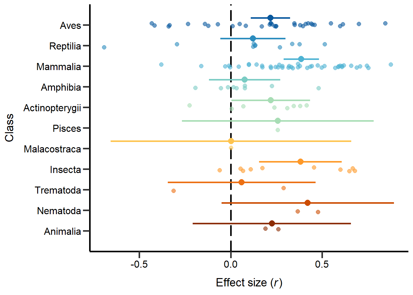
Figure 1: Phylogeny based on classes including sample sizes for the number of studies and number of effect sizes, respectively, and estimates with 95%CI from non-phylogenetic model.
| Version | Author | Date |
|---|---|---|
| 8edd942 | LennartWinkler | 2023-05-01 |
Type of SSD measure
Next we explored the effect of the type of SSD measure (i.e. body mass or size):
MetaData$SSD_Proxy=as.factor(MetaData$SSD_Proxy)
MetaData$SSD_Proxy=relevel(MetaData$SSD_Proxy,c("Body mass"))
Model_REML_by_cSSDMeasure = rma.mv(r ~ SSD_Proxy, V=Var_r, data = MetaData, random = c(~ 1 | Study_ID,~ 1 | Index), method = "REML")
summary(Model_REML_by_cSSDMeasure)
Multivariate Meta-Analysis Model (k = 120; method: REML)

  logLik  Deviance       AIC       BIC      AICc
-23.8130   47.6260   55.6260   66.7088   55.9800

Variance Components:

            estim    sqrt  nlvls  fixed    factor
sigma^2.1  0.0266  0.1632     72     no  Study_ID
sigma^2.2  0.0478  0.2187    120     no     Index

Test for Residual Heterogeneity:
QE(df = 118) = 1511.0606, p-val < .0001

Test of Moderators (coefficient 2):
QM(df = 1) = 4.1937, p-val = 0.0406

Model Results:

                    estimate      se     zval    pval    ci.lb    ci.ub
intrcpt               0.3357  0.0455   7.3733  <.0001   0.2464   0.4249  ***
SSD_ProxyBody size   -0.1221  0.0596  -2.0478  0.0406  -0.2390  -0.0052    *

---
Signif. codes:  0 '***' 0.001 '**' 0.01 '*' 0.05 '.' 0.1 ' ' 1
We then re-leveled the model for post-hoc comparisons:
MetaData$SSD_Proxy=relevel(MetaData$SSD_Proxy,c("Body size"))
Model_REML_by_cSSDMeasure2 = rma.mv(r ~ SSD_Proxy, V=Var_r, data = MetaData, random = c(~ 1 | Study_ID,~ 1 | Index), method = "REML")
summary(Model_REML_by_cSSDMeasure2)
Finally, we computed FDR corrected p-values:
tab3=as.data.frame(round(p.adjust(c(.0001, .0001), method = 'fdr'),digit=3),row.names=cbind("Body mass","Body size"))
colnames(tab3)<-cbind('P-value')
tab3
P-value
Body mass 0
Body size 0SSD measure controlled for body size?
Next we explored the effect if the primary study controlled the SSD for body size (i.e. uncontrolled or controlled):
MetaData$BodySizeControlled=as.factor(MetaData$BodySizeControlled)
MetaData$BodySizeControlled=relevel(MetaData$BodySizeControlled,c("No"))
Model_REML_by_cBodySizeCont = rma.mv(r ~ BodySizeControlled, V=Var_r, data = MetaData, random = c(~ 1 | Study_ID,~ 1 | Index), method = "REML")
summary(Model_REML_by_cBodySizeCont)
Multivariate Meta-Analysis Model (k = 122; method: REML)

  logLik  Deviance       AIC       BIC      AICc
-24.8368   49.6736   57.6736   68.8236   58.0214

Variance Components:

            estim    sqrt  nlvls  fixed    factor
sigma^2.1  0.0309  0.1759     73     no  Study_ID
sigma^2.2  0.0463  0.2152    122     no     Index

Test for Residual Heterogeneity:
QE(df = 120) = 1555.0586, p-val < .0001

Test of Moderators (coefficient 2):
QM(df = 1) = 0.9645, p-val = 0.3261

Model Results:

                       estimate      se     zval    pval    ci.lb   ci.ub
intrcpt                  0.2803  0.0348   8.0595  <.0001   0.2121  0.3485  ***
BodySizeControlledYes   -0.0868  0.0884  -0.9821  0.3261  -0.2600  0.0864

---
Signif. codes:  0 '***' 0.001 '**' 0.01 '*' 0.05 '.' 0.1 ' ' 1
We then re-leveled the model for post-hoc comparisons:
MetaData$BodySizeControlled=relevel(MetaData$BodySizeControlled,c("Yes"))
Model_REML_by_cBodySizeCont2 = rma.mv(r ~ BodySizeControlled, V=Var_r, data = MetaData, random = c(~ 1 | Study_ID,~ 1 | Index), method = "REML")
summary(Model_REML_by_cBodySizeCont2)
Finally, we computed FDR corrected p-values:
tab4=as.data.frame(round(p.adjust(c(.0001, 0.0172), method = 'fdr'),digit=3),row.names=cbind("uncontrolled","controlled"))
colnames(tab4)<-cbind('P-value')
tab4
P-value
uncontrolled 0.000
controlled 0.017Phylogentic vs non-phylogenetic studies
Next we explored the effect of studies controlling for phylogeny vs non-phylogenetic studies:
MetaData$PhyloControlled=as.factor(MetaData$PhyloControlled)
MetaData$PhyloControlled=relevel(MetaData$PhyloControlled,c("No"))
Model_cREML_by_cPhylo = rma.mv(r ~ PhyloControlled, V=Var_r, data = MetaData, random = c(~ 1 | Study_ID,~ 1 | Index), method = "REML")
summary(Model_cREML_by_cPhylo)
Multivariate Meta-Analysis Model (k = 122; method: REML)

  logLik  Deviance       AIC       BIC      AICc
-22.1062   44.2124   52.2124   63.3624   52.5603

Variance Components:

            estim    sqrt  nlvls  fixed    factor
sigma^2.1  0.0230  0.1515     73     no  Study_ID
sigma^2.2  0.0485  0.2202    122     no     Index

Test for Residual Heterogeneity:
QE(df = 120) = 1350.6816, p-val < .0001

Test of Moderators (coefficient 2):
QM(df = 1) = 6.8163, p-val = 0.0090

Model Results:

                    estimate      se     zval    pval    ci.lb    ci.ub
intrcpt               0.4465  0.0759   5.8802  <.0001   0.2977   0.5953  ***
PhyloControlledYes   -0.2163  0.0828  -2.6108  0.0090  -0.3786  -0.0539   **

---
Signif. codes:  0 '***' 0.001 '**' 0.01 '*' 0.05 '.' 0.1 ' ' 1
We then re-leveled the model for post-hoc comparisons:
MetaData$PhyloControlled=relevel(MetaData$PhyloControlled,c("Yes"))
Model_cREML_by_cPhylo2 = rma.mv(r ~ PhyloControlled, V=Var_r, data = MetaData, random = c(~ 1 | Study_ID,~ 1 | Index), method = "REML")
summary(Model_cREML_by_cPhylo2)
Finally, we computed FDR corrected p-values:
tab5=as.data.frame(round(p.adjust(c(0.0001, 0.0001), method = 'fdr'),digit=3),row.names=cbind("Non-phylogenetic","With phylogeny"))
colnames(tab5)<-cbind('P-value')
tab5
P-value
Non-phylogenetic 0
With phylogeny 0Percentage of species with female-biased SSD
Model_cREML_SSbias         = rma.mv(r ~ SSD_SexBias_in_perc_F, V=Var_r, data = MetaData, random = c(~ 1 | Study_ID,~ 1 | Index), method = "REML")
summary(Model_cREML_SSbias)
Multivariate Meta-Analysis Model (k = 104; method: REML)

  logLik  Deviance       AIC       BIC      AICc
-21.0804   42.1607   50.1607   60.6606   50.5731

Variance Components:

            estim    sqrt  nlvls  fixed    factor
sigma^2.1  0.0315  0.1775     64     no  Study_ID
sigma^2.2  0.0465  0.2157    104     no     Index

Test for Residual Heterogeneity:
QE(df = 102) = 1443.6764, p-val < .0001

Test of Moderators (coefficient 2):
QM(df = 1) = 4.8150, p-val = 0.0282

Model Results:

                       estimate      se     zval    pval    ci.lb    ci.ub
intrcpt                  0.3818  0.0550   6.9477  <.0001   0.2741   0.4895  ***
SSD_SexBias_in_perc_F   -0.0023  0.0011  -2.1943  0.0282  -0.0044  -0.0003    *

---
Signif. codes:  0 '***' 0.001 '**' 0.01 '*' 0.05 '.' 0.1 ' ' 1
Test for publication bias
Model_cREML_PublBias         = rma.mv(z ~ SE_z, V=rep(((mean(SE_z)*mean(SE_z))*N),length(SE_z)), data = MetaData, random = c(~ 1 | Study_ID,~ 1 | Index), method = "REML")
summary(Model_cREML_PublBias)
Multivariate Meta-Analysis Model (k = 122; method: REML)

   logLik   Deviance        AIC        BIC       AICc
-145.5101   291.0202   299.0202   310.1702   299.3680

Variance Components:

            estim    sqrt  nlvls  fixed    factor
sigma^2.1  0.0000  0.0000     73     no  Study_ID
sigma^2.2  0.0000  0.0000    122     no     Index

Test for Residual Heterogeneity:
QE(df = 120) = 19.2579, p-val = 1.0000

Test of Moderators (coefficient 2):
QM(df = 1) = 1.5648, p-val = 0.2110

Model Results:

         estimate      se    zval    pval    ci.lb   ci.ub
intrcpt    0.1715  0.1977  0.8678  0.3855  -0.2159  0.5590
SE_z       0.8181  0.6540  1.2509  0.2110  -0.4637  2.0999

---
Signif. codes:  0 '***' 0.001 '**' 0.01 '*' 0.05 '.' 0.1 ' ' 1
Publication year
Next we explored the effect of the publication year of each study:
Model_cREML_by_Year = rma.mv(r ~ Year, V=Var_r, data = MetaData, random = c(~ 1 | Study_ID,~ 1 | Index), method = "REML")
summary(Model_cREML_by_Year)
Multivariate Meta-Analysis Model (k = 122; method: REML)

  logLik  Deviance       AIC       BIC      AICc
-22.8685   45.7371   53.7371   64.8871   54.0849

Variance Components:

            estim    sqrt  nlvls  fixed    factor
sigma^2.1  0.0281  0.1677     73     no  Study_ID
sigma^2.2  0.0453  0.2129    122     no     Index

Test for Residual Heterogeneity:
QE(df = 120) = 1275.7703, p-val < .0001

Test of Moderators (coefficient 2):
QM(df = 1) = 5.0616, p-val = 0.0245

Model Results:

         estimate      se     zval    pval    ci.lb    ci.ub
intrcpt   12.3544  5.3730   2.2994  0.0215   1.8236  22.8853  *
Year      -0.0060  0.0027  -2.2498  0.0245  -0.0113  -0.0008  *

---
Signif. codes:  0 '***' 0.001 '**' 0.01 '*' 0.05 '.' 0.1 ' ' 1
Forest plot
# Sort data by Class
MetaData$Class=as.factor(MetaData$Class)
MetaData$Class=factor(MetaData$Class, levels = c("Animalia","Nematoda","Trematoda","Insecta","Malacostraca","Pisces" ,"Actinopterygii","Amphibia","Mammalia","Reptilia","Aves"))
MetaData_sorted <-MetaData[order(MetaData$r,decreasing = T),]
MetaData_sorted$Class[MetaData_sorted$Class=='Pisces']='Actinopterygii'
MetaData_sorted <-MetaData_sorted[order(MetaData_sorted$Class),]

# Add global effect size to data
forestData=MetaData_sorted[,c(3,5,10,15,18,19)]
forestData[,c(4:6)]=lapply(forestData[,c(4:6)],as.numeric)
forestData$SexSel_Episode=as.factor(forestData$SexSel_Episode)
forestData$SexSel_Episode=factor(forestData$SexSel_Episode, levels = c("pre-copulatory","post-copulatory" ,"both"))
Figure 2
ggplot(data=forestData, aes(y=1:nrow(forestData), x=r, xmin=lCI, xmax=uCI,color=Class,shape=SexSel_Episode,fill=SexSel_Episode)) +
  geom_vline(xintercept=Model_REML_Null$b[1,1], color='black', linetype='solid', alpha=.9,linewidth=0.75)+
  annotate("rect", xmin = Model_REML_Null$ci.lb[1], xmax = Model_REML_Null$ci.ub[1], ymin = 1, ymax = nrow(forestData),alpha = .25)+
geom_vline(xintercept=0, color='black', linetype='dashed', alpha=.5,linewidth=0.8) +
  geom_errorbarh(height=0,size = ifelse(1:nrow(forestData) == c(1), 3.3, 3.3), alpha=1,colour='white')+
  geom_errorbarh(height=0,size = ifelse(1:nrow(forestData) == c(1), 3.3, 3.3), alpha=1)+
  geom_point(size = ifelse(1:nrow(forestData) == c(1), 2, 2), alpha=1,stroke=1,colour='white')+
  geom_point(size = ifelse(1:nrow(forestData) == c(1), 2, 2), alpha=1,stroke=1,colour='black')+
  scale_y_continuous(breaks=seq(1, nrow(forestData), by=1), labels=forestData$AuthorsAndYear,limits=c(1,length(forestData$AuthorsAndYear)),expand=c(0.015,0.015)) +
  labs(title='', x=expression(paste(italic("r "),'(95% CI)')), y = 'Study') +
  theme_classic()+theme(axis.text.x=element_text(size=12),
                        axis.title=element_text(size=12))+ labs(fill =  c("Sexual selection episode"),shape =  c("Sexual selection mode"))+
  scale_colour_manual(values=colpal6, labels=NULL,guide = "none")+
  scale_shape_manual(values=c(21,21,21) ,labels=c("Pre-copulatory","Post-copulatory" ,"Both"))+
  scale_fill_manual(values=c('grey50','white','black'),labels=c("Pre-copulatory","Post-copulatory" ,"Both"))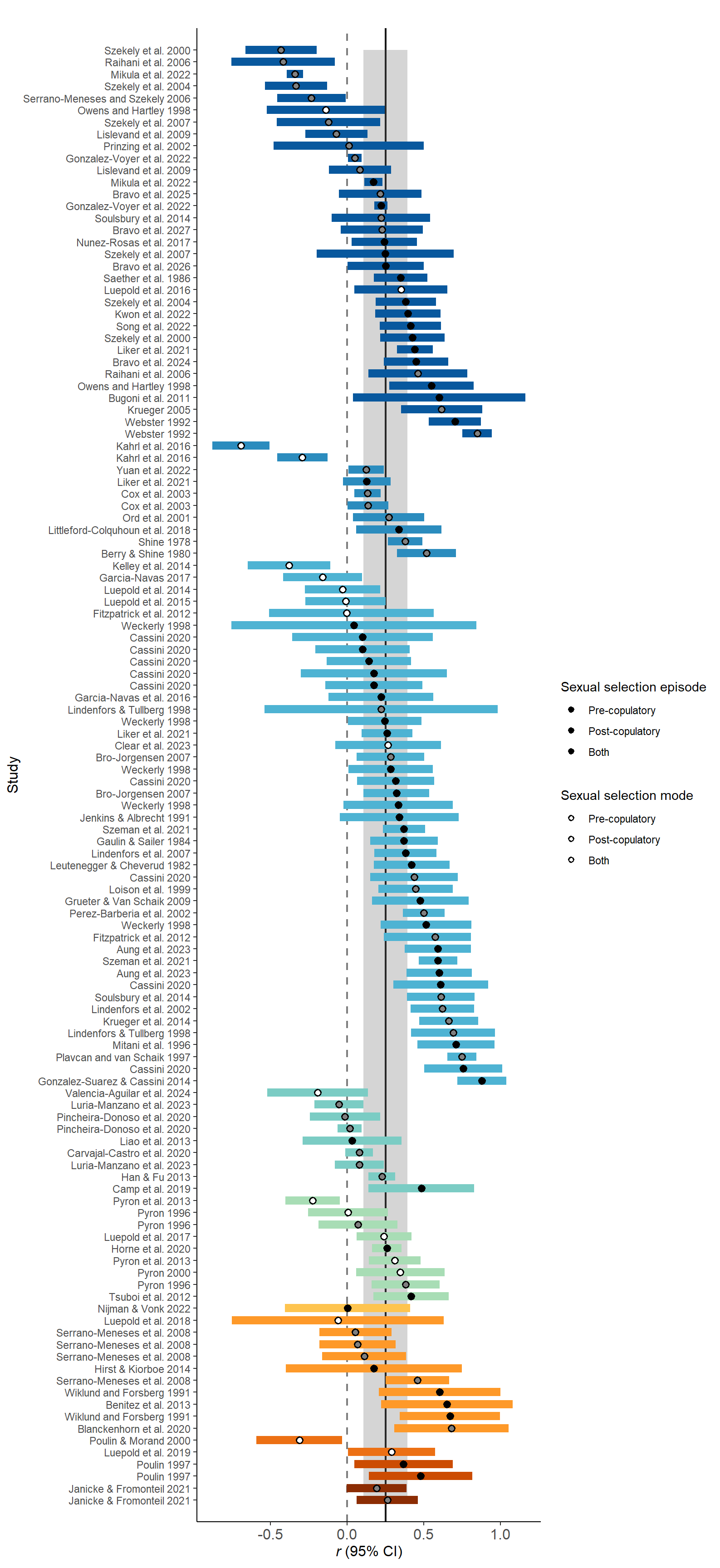
Figure 2: Forest plot including correlation coefficients (±95% CI), as well as the global effect size (in grey) with and without controlling for phylogeny. Different animal classes highlighted by background colors (see Figure 1 for class names) and sexual selection modes pre- (red), post-copulatory (blue) and both (green) by color of effect size.
| Version | Author | Date |
|---|---|---|
| 054a12b | LennartWinkler | 2023-04-30 |
R version 4.3.3 (2024-02-29 ucrt)
Platform: x86_64-w64-mingw32/x64 (64-bit)
Running under: Windows 10 x64 (build 19045)

Matrix products: default


locale:
[1] LC_COLLATE=German_Germany.utf8  LC_CTYPE=German_Germany.utf8
[3] LC_MONETARY=German_Germany.utf8 LC_NUMERIC=C
[5] LC_TIME=German_Germany.utf8

time zone: Europe/Berlin
tzcode source: internal

attached base packages:
[1] stats     graphics  grDevices utils     datasets  methods   base

other attached packages:
 [1] gridExtra_2.3       wesanderson_0.3.7   PupillometryR_0.0.5
 [4] rlang_1.1.3         dplyr_1.1.4         cowplot_1.1.3
 [7] ggdist_3.3.2        MCMCglmm_2.35       coda_0.19-4.1
[10] RColorBrewer_1.1-3  ggplot2_3.5.0       data.table_1.15.2
[13] multcomp_1.4-25     TH.data_1.1-2       survival_3.5-8
[16] mvtnorm_1.2-4       psych_2.4.3         pwr_1.3-0
[19] MASS_7.3-60.0.1     metafor_4.4-0       numDeriv_2016.8-1.1
[22] metadat_1.2-0       Matrix_1.6-5        matrixcalc_1.0-6
[25] ape_5.7-1           workflowr_1.7.1

loaded via a namespace (and not attached):
 [1] tidyselect_1.2.1     farver_2.1.1         fastmap_1.1.1
 [4] tensorA_0.36.2.1     mathjaxr_1.6-0       promises_1.2.1
 [7] digest_0.6.35        lifecycle_1.0.4      processx_3.8.4
[10] magrittr_2.0.3       compiler_4.3.3       sass_0.4.9
[13] tools_4.3.3          utf8_1.2.4           yaml_2.3.8
[16] knitr_1.45           labeling_0.4.3       mnormt_2.1.1
[19] withr_3.0.0          purrr_1.0.2          grid_4.3.3
[22] fansi_1.0.6          git2r_0.33.0         colorspace_2.1-0
[25] scales_1.3.0         cli_3.6.1            rmarkdown_2.26
[28] generics_0.1.3       rstudioapi_0.16.0    httr_1.4.7
[31] cachem_1.0.8         stringr_1.5.1        splines_4.3.3
[34] parallel_4.3.3       vctrs_0.6.5          sandwich_3.1-0
[37] jsonlite_1.8.8       callr_3.7.5          jquerylib_0.1.4
[40] tidyr_1.3.1          glue_1.7.0           codetools_0.2-19
[43] ps_1.7.6             distributional_0.4.0 stringi_1.8.3
[46] cubature_2.1.0       gtable_0.3.4         later_1.3.2
[49] munsell_0.5.0        tibble_3.2.1         pillar_1.9.0
[52] htmltools_0.5.7      R6_2.5.1             rprojroot_2.0.4
[55] evaluate_0.23        lattice_0.22-5       highr_0.10
[58] corpcor_1.6.10       httpuv_1.6.14        bslib_0.6.1
[61] Rcpp_1.0.12          nlme_3.1-164         whisker_0.4.1
[64] xfun_0.42            fs_1.6.3             zoo_1.8-12
[67] getPass_0.2-4        pkgconfig_2.0.3