Differential Gene Expression with DESeq2 and edgeR
Maeva Techer
2025-01-13
Last updated: 2025-01-13
Checks: 7 0
Knit directory:
locust-comparative-genomics/
This reproducible R Markdown analysis was created with workflowr (version 1.7.1). The Checks tab describes the reproducibility checks that were applied when the results were created. The Past versions tab lists the development history.
Great! Since the R Markdown file has been committed to the Git repository, you know the exact version of the code that produced these results.
Great job! The global environment was empty. Objects defined in the global environment can affect the analysis in your R Markdown file in unknown ways. For reproduciblity it’s best to always run the code in an empty environment.
The command set.seed(20221025) was run prior to running
the code in the R Markdown file. Setting a seed ensures that any results
that rely on randomness, e.g. subsampling or permutations, are
reproducible.
Great job! Recording the operating system, R version, and package versions is critical for reproducibility.
Nice! There were no cached chunks for this analysis, so you can be confident that you successfully produced the results during this run.
Great job! Using relative paths to the files within your workflowr project makes it easier to run your code on other machines.
Great! You are using Git for version control. Tracking code development and connecting the code version to the results is critical for reproducibility.
The results in this page were generated with repository version 6954b9b. See the Past versions tab to see a history of the changes made to the R Markdown and HTML files.
Note that you need to be careful to ensure that all relevant files for
the analysis have been committed to Git prior to generating the results
(you can use wflow_publish or
wflow_git_commit). workflowr only checks the R Markdown
file, but you know if there are other scripts or data files that it
depends on. Below is the status of the Git repository when the results
were generated:
Ignored files:
    Ignored:    .DS_Store
    Ignored:    analysis/.DS_Store
    Ignored:    data/.DS_Store
    Ignored:    data/DEG-results/.DS_Store
    Ignored:    data/WGCNA_input/.DS_Store
    Ignored:    data/WGCNA_output/.DS_Store
    Ignored:    data/behavioral_data/.DS_Store
    Ignored:    data/behavioral_data/Raw_data/.DS_Store
    Ignored:    data/list/.DS_Store
    Ignored:    data/list/GO_Annotations/.DS_Store
    Ignored:    data/orthofinder/.DS_Store
    Ignored:    data/orthofinder/Polyneoptera/.DS_Store
    Ignored:    data/orthofinder/Polyneoptera/Orthogroups/.DS_Store
    Ignored:    data/orthofinder/Schistocerca/.DS_Store
    Ignored:    data/orthofinder/Schistocerca/Orthogroups/.DS_Store

Untracked files:
    Untracked:  data/orthofinder/Polyneoptera/Orthogroups/Orthogroups.tsv
    Untracked:  data/orthofinder/Polyneoptera/Orthogroups/Orthogroups.txt
    Untracked:  data/orthofinder/Polyneoptera/Orthogroups/Orthogroups_reprocessed.tsv
    Untracked:  data/orthofinder/Polyneoptera/Orthogroups/Orthogroups_reprocessed.txt
    Untracked:  data/orthofinder/Schistocerca/Orthogroups/Orthogroups.tsv
    Untracked:  data/orthofinder/Schistocerca/Orthogroups/Orthogroups.txt
    Untracked:  data/orthofinder/Schistocerca/Orthogroups/Orthogroups_reprocessed.tsv
    Untracked:  data/orthofinder/Schistocerca/Orthogroups/Orthogroups_reprocessed.txt

Unstaged changes:
    Modified:   analysis/1_research-questions.Rmd
    Modified:   analysis/1_seq-data.Rmd
    Modified:   analysis/1_team-science.Rmd
    Modified:   analysis/1_workenvs-prep.Rmd
    Modified:   analysis/2_gene-family.Rmd
    Modified:   analysis/2_hypotheses.Rmd
    Modified:   analysis/2_orthologs-prediction.Rmd
    Deleted:    analysis/2_repeat-landscape 2.Rmd
    Modified:   analysis/2_repeat-landscape.Rmd
    Modified:   analysis/2_synteny-graphs.Rmd
Note that any generated files, e.g. HTML, png, CSS, etc., are not included in this status report because it is ok for generated content to have uncommitted changes.
These are the previous versions of the repository in which changes were
made to the R Markdown (analysis/3_deg-analysis.Rmd) and
HTML (docs/3_deg-analysis.html) files. If you’ve configured
a remote Git repository (see ?wflow_git_remote), click on
the hyperlinks in the table below to view the files as they were in that
past version.
| File | Version | Author | Date | Message |
|---|---|---|---|---|
| html | 3fa8e62 | Maeva TECHER | 2024-11-09 | updated analysis |
| html | edb70fe | Maeva TECHER | 2024-11-08 | overlap and deg results created |
| html | 7f1d1fe | Maeva TECHER | 2024-11-01 | Build site. |
| Rmd | f01f1cf | Maeva TECHER | 2024-11-01 | Adding new files and docs |
| html | f01f1cf | Maeva TECHER | 2024-11-01 | Adding new files and docs |
| html | ba35b82 | Maeva A. TECHER | 2024-06-20 | Build site. |
| html | e34a3b8 | Maeva A. TECHER | 2024-05-16 | Build site. |
| Rmd | 3f5566f | Maeva A. TECHER | 2024-05-16 | wflow_publish("analysis/3_deg-analysis.Rmd") |
| html | e9d8b9a | Maeva A. TECHER | 2024-05-16 | Build site. |
| Rmd | 3fd7172 | Maeva A. TECHER | 2024-05-16 | wflow_publish("analysis/3_deg-analysis.Rmd") |
| html | 5b7e6d5 | Maeva A. TECHER | 2024-05-15 | Build site. |
| Rmd | 0ac8380 | Maeva A. TECHER | 2024-05-15 | wflow_publish("analysis/3_deg-analysis.Rmd") |
| html | da47a64 | Maeva A. TECHER | 2024-05-15 | Build site. |
| html | a39899b | Maeva A. TECHER | 2024-05-15 | Build site. |
| Rmd | b02e6e9 | Maeva A. TECHER | 2024-05-15 | wflow_publish("analysis/3_deg-analysis.Rmd") |
| html | e39d280 | Maeva A. TECHER | 2024-01-30 | Build site. |
| html | f701a01 | Maeva A. TECHER | 2024-01-30 | reupdate |
| html | a3d138b | Maeva A. TECHER | 2024-01-30 | Build site. |
| Rmd | 915285e | Maeva A. TECHER | 2024-01-30 | wflow_publish("analysis/3_deg-analysis.Rmd") |
| html | 959a4e9 | Maeva A. TECHER | 2024-01-24 | Build site. |
| html | 1b09cbe | Maeva A. TECHER | 2024-01-24 | remove |
| html | 478e72d | Maeva A. TECHER | 2023-12-18 | Build site. |
| Rmd | 53877fa | Maeva A. TECHER | 2023-12-18 | add pages |
Here we present the workflow example with the head data from S. piceifrons mapped to its own genome. We applied the same process for each species ( S. americana, S. serialis cubense, S. nitens, S. gregaria, S. cancellata and S. piceifrons), tissue (head or thorax) and each mapping strategy (mapped to shared gregaria Ref Seq or own Ref Seq). The results can be seen in the DEG results section.
For the analysis of differentially expressed genes, we will follow
some guidelines from an online RNA course tutorial
that uses either DESeq2 or edgeR on STAR
output. We also adapted some script lines from Foquet et
al. 2021 code. For each workflow, we also present the
“lazy” method when we want quick results and the
“step-by-step” method where we tailored in real time
our thresholds. Our aim will be to
combine both results and take only the overlapping DEGs detected by
these two software.
Both DESeq2 and edgeR identify
differentially expressed genes by starting with the hypothesis that no
genes are differentially expressed. They work similarly but differs
slightly in the normalization process. Where DEseq2 use a
“geometric” normalization, edgeR uses a weighted mean of
log ratios-based method. If you want to understand the process and
algorithms for each of these R package, I recommend to check their
bioconductor page.
Warning: For sample size over 8 per condition, please be aware that both methods have been found to overestimate DEGs with false positive in human population samples. You can read more about it with Li et al. 2022.
For example purpose, we will compare here the transcriptomes from head tissues of S. piceifrons specimens reared in isolated and crowded conditions.
1. Preparing input files
Raw count matrices
We generated this in the STAR mapping section.
Transcript-to-gene annotation file
We need to format the .gtf annotation file for input in both
DESeq2 and edgeR if we need annotation.
Below is the example with S. piceifrons
# Download annotation and place it into the folder refgenomes
wget https://ftp.ncbi.nlm.nih.gov/genomes/all/GCF/021/461/385/GCF_021461385.2_iqSchPice1.1/GCF_021461385.2_iqSchPice1.1_genomic.gtf.gz

# first column is the transcript ID, second column is the gene ID, third column is the gene symbol
zcat GCF_021461385.2_iqSchPice1.1_genomic.gtf.gz | awk -F "\t" 'BEGIN{OFS="\t"}{if($3=="transcript"){split($9, a, "\""); print a[4],a[2],a[8]}}' > tx2gene.piceifrons.csv
The alternative is a python script developed by David to parse the .gff.
import regex as re

filename = "xpApisu.gff"
outfile = 'gffKeyApisu.tsv'
lol = {}
with open(filename) as gffFile:
    for line in gffFile:
        if re.search(r"product=[^;]+", line):
            gene = re.search(r"gene=[^;=]+", line)
            gene = gene.group(0)
            if gene.endswith('product'):
                gene = gene[5:-7]
            else:
                gene = gene[5:]
            product = re.search(r"product=[^;]+", line)
            product = product.group(0)
            product = product.replace("product=", "")
            product = product.rstrip()
            proteinID = re.search(r"protein_id=(.+)", line)
            proteinID = proteinID.group(1)
            if proteinID not in lol.keys():
                lol[proteinID] = [gene, product]
with open(outfile, 'w') as output:
    for proID,lis in lol.items():
        output.writelines(proID + '\t' + lis[0] + '\t' + lis[1] + '\n')
Sample sheet
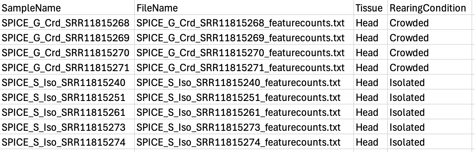
DESeq2 and edgeR need a sample sheet that
describes the samples characteristics: SampleName, FileName
(…counts.txt), and subsequently anything that can be used for
statistical design such as RearingCondition,
replicates, tissue, time points, etc. in the form.
The design indicates how to model the samples: in the model we need to specify what we want to measure and what we want to control.
Reference state
For all our subsequent analysis, we will consider the
RearingCondition Isolated or the Phase
Solitarious to be the reference baseline state
(condRef) In nature, swarming are usually episodic and it
is more frequent to encounter solitarious phenotypes (Tanaka
and Nishide, 2013, Barrientos-Lozano et
al., 2021). This means that up and down regulated genes are in
Crowded or Gregarious phase compared
to Isolated to Solitarious.
2. DESeq2 analysis using STAR input
2.1. Load libraries
We start by loading all the required R packages.
#(install first from CRAN or Bioconductor)
library("DESeq2")
library("tximport")
library("txdbmaker")
library("knitr")
library("rmdformats")
library("tidyverse")
library("data.table")
library("DT")  # for making interactive search table
library("plotly") # for interactive plots
library("ggthemes") # for theme_calc
library("reshape2")
library("ComplexHeatmap")
library("RColorBrewer")
library("circlize")
library("apeglm")
library("ggpubr")
library("ggplot2")
library("ggrepel")
library("EnhancedVolcano")
library("SARTools")
library("pheatmap")
library("clusterProfiler")
library("sva")
library("cowplot")
library("ashr")
library("ggConvexHull")
2.2. Lazy DEG analysis
Here we will be using the html report function of DESeq2
to export all the results, however, the option to do it step by step
will be also provided below.
Set parameters
We need to specify the path of our working directories, where are located our gene counts files and where the .html report will be created:
## PARAMETERS for running the script
homeDir <- "{PATH TO YOUR FOLDER}/locust-comparative-genomics"
workDir <- "{PATH TO YOUR FOLDER}/locust-comparative-genomics/data"     # Working directory

# path to the directory containing raw counts files
rawDir <- file.path(workDir, "03-{species}-DESeq2")

## Details to create the html report
projectName <- "SPECIESXXX_HEAD"                # name of the project
author <- "Maeva TECHER"                        # author of the statistical analysis/report

## Create all the needed directories for the html report
setwd(workDir)
Dirname <- paste("DEseq2_", projectName, sep = "")
dir.create(Dirname)
setwd(Dirname)
workDir_DEseq2 <- getwd()
We then define the parameters that we will be running with
DESeq2. We will choose the solitarious
phase or isolated condition to be our reference for all
analysis.
## PARAMETERS for running DEseq2
tresh_logfold <- 1                            # Treshold for log2(foldchange) in final DE-files
tresh_padj <- 0.05                            # Treshold for adjusted p-valued in final DE-files
alpha_DEseq2 <- 0.05                  # threshold of statistical significance
pAdjustMethod_DEseq2 <- "BH"          # p-value adjustment method: "BH" (default) or "BY"
featuresToRemove <- c(NULL)           # names of the features to be removed, NULL if none or if using Idxstats
varInt <- "RearingCondition"          # factor of interest
condRef <- "Isolated"                 # reference biological condition Isolated
batch <- NULL                         # blocking factor: NULL (default) or "batch" for example
fitType <- "parametric"               # mean-variance relationship: "parametric" (default) or "local"
cooksCutoff <- TRUE                   # TRUE/FALSE to perform the outliers detection (default is TRUE)
independentFiltering <- TRUE          # TRUE/FALSE to perform independent filtering (default is TRUE)
typeTrans <- "rlog"                   # transformation for PCA/clustering: "VST" or "rlog"
locfunc <- "median"

# Path and name of targetfile containing conditions and file names
species <- "piceifrons"  # Example species
targetFile <- file.path(workDir, "list", paste0("Head", "_", species, ".txt"))

colors <- c("#B31B21", "#1465AC", "green3", "orange")
Here our targetFile is our metadata which should have a
column for each: sample ID, the file name (exactly the same as in your
folder, be careful with ” ” or “_”) and the conditions. Below we show an
example with the files for piceifrons head:
If everything has been loaded properly, the next chunk of code should not show any warning and we can simply proceed to the actual DEG analysis.
# checking parameters
setwd(workDir_DEseq2)

checkParameters.DESeq2(projectName=projectName,author=author,targetFile=targetFile,
                       rawDir=rawDir,featuresToRemove=featuresToRemove,varInt=varInt,
                       condRef=condRef,batch=batch,fitType=fitType,cooksCutoff=cooksCutoff,
                       independentFiltering=independentFiltering,alpha=alpha_DEseq2,pAdjustMethod=pAdjustMethod_DEseq2,
                       typeTrans=typeTrans,locfunc=locfunc,colors=colors)
Create the HTML report
Here if you just want a quick report without being able to tailor step by step, you can use the code below and obtain several graphs and details for your DEG analysis.
## import the sample sheet that indicates Rearing Conditions and Tissue origins
setwd(workDir_DEseq2)

# loading target file
target <- loadTargetFile(targetFile=targetFile, varInt=varInt, condRef=condRef, batch=batch)

# loading counts
counts <- loadCountData(target=target, rawDir=rawDir, featuresToRemove=featuresToRemove)

# description plots
majSequences <- descriptionPlots(counts=counts, group=target[,varInt], col=colors)

# analysis with DESeq2
out.DESeq2 <- run.DESeq2(counts=counts, target=target, varInt=varInt, batch=batch,
                         locfunc=locfunc, fitType=fitType, pAdjustMethod=pAdjustMethod_DEseq2,
                         cooksCutoff=cooksCutoff, independentFiltering=independentFiltering, alpha=alpha_DEseq2)

# PCA + Clustering
exploreCounts(object=out.DESeq2$dds, group=target[,varInt], typeTrans=typeTrans, col=colors)

# summary of the analysis (boxplots, dispersions, diag size factors, export table, nDiffTotal, histograms, MA plot)
summaryResults <- summarizeResults.DESeq2(out.DESeq2, group=target[,varInt], col=colors,
                                          independentFiltering=independentFiltering,
                                          cooksCutoff=cooksCutoff, alpha=alpha_DEseq2)

# generating HTML report
writeReport.DESeq2(target=target, counts=counts, out.DESeq2=out.DESeq2, summaryResults=summaryResults,
                   majSequences=majSequences, workDir=workDir_DEseq2, projectName=projectName, author=author,
                   targetFile=targetFile, rawDir=rawDir, featuresToRemove=featuresToRemove, varInt=varInt,
                   condRef=condRef, batch=batch, fitType=fitType, cooksCutoff=cooksCutoff,
                   independentFiltering=independentFiltering, alpha=alpha_DEseq2, pAdjustMethod=pAdjustMethod_DEseq2,
                   typeTrans=typeTrans, locfunc=locfunc, colors=colors)
2.3. Step-by-step DEG analysis
Set parameters
Here we only need to specify the path of our raw counts and metadata files.
## PARAMETERS for running the script
workDir <- "{PATH TO YOUR FOLDER}/locust-comparative-genomics/data" # Working directory

# path to the directory containing raw counts files
rawDir <- file.path(workDir, "03-{species}-DESeq2")
We then import the metadata table and format it as such as there is no error downstream.
# Get in the home directory and load the file of interest
setwd(workDir)
sampletable <- fread("list/HeadSAMER_nooutliers.txt")

## add the sample names as row names (it is needed for some of the DESeq functions)
rownames(sampletable) <- sampletable$SampleName

## Make sure discriminant variables are factor
sampletable$RearingCondition <- as.factor(sampletable$RearingCondition)
sampletable$Tissue <- as.factor(sampletable$Tissue)

dim(sampletable)
If you need to have the correspondance between transcript and Gene_ID (as for SALMON) we need to create the gene database.
### Create tx2gene file  ######
txdb <- makeTxDbFromGFF("annotation/GCF_021461395.2_iqSchAmer2.1_genomic.gtf")
k <- keys(txdb, keytype = "TXNAME")
tx2gene <- AnnotationDbi::select(txdb, k, "GENEID", "TXNAME")
Then we obtain the output from STAR GeneCount and import
here individually using the sampletable as a reference to
fetch them. We also filter the lowly expressed genes to avoid noisy
data.
## Import count files
satoshi <- DESeqDataSetFromHTSeqCount(sampleTable = sampletable,
                        directory = rawDir,
                        design = ~ RearingCondition )
satoshi

# Pre-filtering
# keep genes for which sums of raw counts across experimental samples is > 5
smallestGroupSize <- 3
keep <- rowSums(counts(satoshi) >= 5) >= smallestGroupSize
satoshi <- satoshi[keep,]
nrow(satoshi)

# Relevel so that Isolated is the baseline status
satoshi$RearingCondition <- relevel(satoshi$RearingCondition, ref = "Isolated")
We then define the parameters that we will be running with
DESeq2:
## PARAMETERS for running DEseq2
tresh_logfold <- 1                            # Treshold for log2(foldchange) in final DE-files
tresh_padj <- 0.05                            # Treshold for adjusted p-valued in final DE-files
alpha_DEseq2 <- 0.05                  # threshold of statistical significance
pAdjustMethod_DEseq2 <- "BH"          # p-value adjustment method: "BH" (default) or "BY"
featuresToRemove <- c(NULL)           # names of the features to be removed, NULL if none or if using Idxstats
varInt <- "RearingCondition"          # factor of interest
condRef <- "Isolated"                 # reference biological condition
batch <- NULL                         # blocking factor: NULL (default) or "batch" for example
fitType <- "parametric"               # mean-variance relationship: "parametric" (default) or "local"
cooksCutoff <- TRUE                   # TRUE/FALSE to perform the outliers detection (default is TRUE)
independentFiltering <- TRUE          # TRUE/FALSE to perform independent filtering (default is TRUE)
typeTrans <- "rlog"                     # transformation for PCA/clustering: "VST" or "rlog"
locfunc <- "median"
Run the model Fit DESeq2
Run DESeq2 analysis using DESeq, which performs (1)
estimation of size factors, (2) estimation of dispersion, then (3)
Negative Binomial GLM fitting and Wald statistics. The results tables
(log2 fold changes and p-values) can be generated using the results
function (copied
from online chapter).
One of the thing we want to do with the step-by-step method is to remove some of special genomic features such as long -non-coding RNA genes or ribosomal RNA. For that we created a list beforehand by parsing the .gff file and selecting field of interest for each species.
IF WE WANT TO EXCLUDE SOME LOCI USE THIS CODE:
# Read the list of loci from a text file to later remove it
loci_to_exclude <- readLines("{PATH TO YOUR FOLDER}/locust-comparative-genomics/data/list/excluded_loci/SPECIESXXX_lncrna_list.txt")

# Subset the rows of the DESeqDataSet to exclude the loci in the 'loci_to_exclude' list
satoshi_filtered <- satoshi[!(rownames(satoshi) %in% loci_to_exclude), ]

shigeru <- DESeq(satoshi_filtered)
cbind(resultsNames(shigeru))
IF WE DO NOT WANT TO EXCLUDE ANY LOCI USE THIS CODE:
# Fit the statistical model
shigeru <- DESeq(satoshi)
cbind(resultsNames(shigeru))
Then we will observe the final result by keeping DEGs with an adjusted p-value cutoff > 0.05.
# Here we plot the adjusted p-value means corrected for multiple testing (FDR padj)
res_shigeru <- results(shigeru)

# We only keep genes with an adjusted p-value cutoff > 0.05 by changing the default significance cut-off
sum(res_shigeru$padj < tresh_padj, na.rm = TRUE)
# To quickly visualize the count reads between condition of the gene with smallest pvalue
plotCounts(shigeru, gene=which.min(res_shigeru$padj), intgroup="RearingCondition")

brock <- results(shigeru, name = "RearingCondition_Isolated_vs_Crowded", alpha = alpha_DEseq2)
summary(brock)

# Details of what is each column meaning in our final result
mcols(brock)$description
head(brock)
2.4. Visualizing and exploring the results
This can be done only with the step-by-step method. The html report can output similar figures but with less possibility for tailoring.
PCA of the samples
We transformed the data for visualization by comparing both recommended rlog (Regularized log) or vst (Variance Stabilizing Transformation) transformations. Both options produce log2 scale data which has been normalized by the DESeq2 method with respect to library size.
# Try with the vst transformation
shigeru_vst <- vst(shigeru)
shigeru_rlog <- rlog(shigeru)
shigeru_ntd <- normTransform(shigeru)

# to test if the transformation is fitting the data
# this gives log2(n + 1)
library("vsn")
itadori <- meanSdPlot(assay(shigeru_ntd))
itadori$gg + ggtitle("Transformation with ntd")
megumi <- meanSdPlot(assay(shigeru_vst))
megumi$gg + ggtitle("Transformation with vst")
nobara <- meanSdPlot(assay(shigeru_rlog))
nobara$gg + ggtitle("Transformation with rlog")
Here we will plot the data using the rlog transformation and PCA approach. Looking at this type of data is a good first method to potentially detect outlier that we may need to remove. These outliers can be created due to library preparation contamination or sequencing errors. We can confirm this suspicion with the QC and expression heatmap analysis to make sure we are not excluding sample that merely display non-artifact variability.
# Create the pca on the defined groups
pcaData1 <- plotPCA(object = shigeru_rlog, intgroup = c("RearingCondition"),returnData=TRUE)

# Store the information for each axis variance in %
percentVar <- round(100 * attr(pcaData1, "percentVar"))

# Make sure that the discriminant variable are in factor for using shape and color later on
pcaData1$RearingCondition<-factor(pcaData1$RearingCondition,levels=c("Crowded","Isolated"), labels=c("Crowded SPECIESXXX","Isolated SPECIESXXX"))
levels(pcaData1$RearingCondition)

library(ggdist)

p1 <- ggplot(pcaData1, aes(PC1, PC2, color= RearingCondition)) +
  geom_point(size=12) +
  xlab(paste0("PC1: ", percentVar[1], "% variance")) +
  ylab(paste0("PC2: ", percentVar[2], "% variance")) +
  scale_color_manual(values = c("blue", "red")) +
  #coord_fixed() +
  theme_bw() +
  theme(legend.title = element_blank()) +
  theme(legend.text = element_text(face="bold", size=24)) +
  theme(axis.text = element_text(size=20)) +
  theme(axis.title = element_text(size=20))

p1 + geom_convexhull(aes(fill = RearingCondition, color = RearingCondition), alpha = 0.5) +
    scale_fill_manual(values = c("blue", "red"))+
    ggtitle("PCA on SPECIESXXX YYY tissues", subtitle = "rlog transformation")
Here we will plot the data using the vst transformation and PCA approach:
# Create the pca on the defined groups
pcaData2 <- plotPCA(object = shigeru_vst, intgroup = c("RearingCondition"),returnData=TRUE)

# Store the information for each axis variance in %
percentVar <- round(100 * attr(pcaData2, "percentVar"))

# Make sure that the discriminant variable are in factor for using shape and color later on
pcaData2$RearingCondition<-factor(pcaData2$RearingCondition,levels=c("Crowded","Isolated"), labels=c("Crowded SPECIESXXX","Isolated SPECIESXXX"))
levels(pcaData2$RearingCondition)


p2 <-ggplot(pcaData2, aes(PC1, PC2, color= RearingCondition)) +
  geom_point(size=12) +
  xlab(paste0("PC1: ", percentVar[1], "% variance")) +
  ylab(paste0("PC2: ", percentVar[2], "% variance")) +
  scale_color_manual(values = c("blue", "red")) +
  #coord_fixed() +
  theme_bw() +
  theme(legend.title = element_blank()) +
  theme(legend.text = element_text(face="bold", size=24)) +
  theme(axis.text = element_text(size=20)) +
  theme(axis.title = element_text(size=20))

p2 + geom_convexhull(aes(fill = RearingCondition, color = RearingCondition), alpha = 0.5) +
    scale_fill_manual(values = c("blue", "red"))+
    ggtitle("PCA on SPECIESXXX YYY tissues", subtitle = "vst transformation")
Heatmap of the count matrix
select <- order(rowMeans(counts(shigeru,normalized=TRUE)),
                decreasing=TRUE)[1:9]
df <- as.data.frame(colData(shigeru)[,c("RearingCondition","Tissue")])
# we normalized the reads and compare the pattens of data transformation
pheatmap(assay(shigeru_ntd)[select,], cluster_rows=FALSE, show_rownames=FALSE,
         cluster_cols=FALSE, annotation_col=df)
pheatmap(assay(shigeru_vst)[select,], cluster_rows=FALSE, show_rownames=FALSE,
         cluster_cols=FALSE, annotation_col=df)
pheatmap(assay(shigeru_rlog)[select,], cluster_rows=FALSE, show_rownames=FALSE,
         cluster_cols=FALSE, annotation_col=df)
Sample Matrix Distance
Using also the transformed data, we check the distance between samples and see how they correlate to each others. We will create a heatmap to look at the expression levels differences and patterns across our samples using the rlog transformation first.
metadata <- sampletable[,c("RearingCondition", "Tissue")]
rownames(metadata) <- sampletable$SampleName

# calculate between-sample distance matrix
sampleDistMatrix.rlog <- as.matrix(dist(t(assay(shigeru_rlog))))

pheatmap(sampleDistMatrix.rlog, annotation_col=metadata, main = "YYY tissue heatmap, rlog transformation")
We can do the same with the vst transformation to see any differences.
# calculate between-sample distance matrix
sampleDistMatrix.vst<- as.matrix(dist(t(assay(shigeru_vst))))

pheatmap(sampleDistMatrix.vst, annotation_col=metadata, main = "YYY tissue heatmap, rlog transformation")
MA-plot
This plot allows us to show the log2 fold changes over the mean of normalized counts for all the samples. Points will be colored in red if the adjusted p-value is less than 0.05 and the log2 fold change is bigger than 1. In blue, will be the reverse with a significant -1 log2 fold change.
To generate more accurate log2 fold change estimates, DESeq2 allows (and recommends) the shrinkage of effect size (the LFC estimates) toward zero when the information for a gene is low, which could include:
- Low counts
- High dispersion values
# include the log2FoldChange shrinkage use to visualize gene ranking
de_shrink <- lfcShrink(dds = shigeru, coef="RearingCondition_Isolated_vs_Crowded", type="apeglm")
head(de_shrink)

# Ma plot parameters
maplot <-ggmaplot(de_shrink, fdr = 0.05, fc = 1, size = 2, palette = c("#B31B21", "#1465AC", "darkgray"), genenames = as.vector(rownames(de_shrink$name)), top = 0,legend="top",label.select = NULL) +
  coord_cartesian(xlim = c(0, 20)) +
  scale_y_continuous(limits=c(-12, 12)) +
  theme(axis.text.x = element_text(size=16),axis.text.y = element_text(size=15),axis.title.x = element_text(size=17),axis.title.y = element_text(size=17),axis.line = element_line(size = 1, colour="gray20"),axis.ticks = element_line(size = 1, colour="gray20")) +
  guides(color = guide_legend(override.aes = list(size = c(3,3,3)))) +
  theme(legend.position = c(0.70, 0.12),legend.text=element_text(size=14,face="bold"),legend.background = element_rect(fill="transparent")) +
  theme(plot.title = element_text(size=18, colour="gray30", face="bold",hjust=0.06, vjust=-5)) +
  labs(title="MA-plot for the shrunken log2 fold changes in the YYY tissues")

maplot
Volcano Plot
The EnhancedVolcano helps visualize the results of the
differential expression analysis. This plot shows for each gene, the
expression log fold change between our isolated and crowded individuals
on the x-axis against the p-value plotted on the y-axis. This is an easy
way to quickly identify extreme changes in genes transcription following
locust phase change.
keyvals <-ifelse(
  res_shigeru$log2FoldChange >= 1 & res_shigeru$padj <= 0.05, '#B31B21',
  ifelse(res_shigeru$log2FoldChange <= -1 & res_shigeru$padj <= 0.05, '#1465AC', 'darkgray'))

keyvals[is.na(keyvals)] <-'darkgray'
names(keyvals)[keyvals == "#B31B21"] <-'Upregulated'
names(keyvals)[keyvals == "#1465AC"] <-'Downregulated'
names(keyvals)[keyvals == 'darkgray'] <-'NS'

EnhancedVolcano(res_shigeru,
                lab = rownames(res_shigeru),
                x = 'log2FoldChange',
                y = 'padj',
                pCutoff = 0.05,
                FCcutoff = 1,
                pointSize = 3,
                labSize = 5,
                colAlpha = 4/5,
                colCustom = keyvals,
                drawConnectors = TRUE)
Normalized Matrix distance
We can reavaluate the distance between our samples by normalizing the results when extracting only genes that had a signficant log fold change of 1. This value can be customized according to the user preference, but for our purposes here we decided to select any changes of expression that at least doubled from our choosen reference condition (i.e., crowded).
resorted_deresults <- res_shigeru[order(res_shigeru$padj),]

## Select only the genes that have a padj > 0.05 and with minimum log2FoldChange of 1
sig <- resorted_deresults[!is.na(resorted_deresults$padj) &
                            resorted_deresults$padj < tresh_padj &
                            abs(resorted_deresults$log2FoldChange) >= 1,]
selected <- rownames(sig);selected

## Norm transform the data from DEseq2 run
ntd <- normTransform(satoshi)

## Plot the relation among samples considering only the significant genes
pheatmap(assay(ntd)[selected,],
         annotation_col=metadata,
         cluster_rows = TRUE,
         show_rownames = TRUE,
         cluster_cols = TRUE,
         cutree_rows = 4,
         cutree_cols = 3,
         labels_col= colData(satoshi)$SampleName)
3. edgeR analysis using STAR input
We followed partially the comprehensive tutorial for edgeR.
3.1. Load libraries
We start by loading all the required R packages.
#(install first from CRAN or Bioconductor)
library("knitr")
library("rmdformats")
library("tidyverse")
library("DT")  # for making interactive search table
library("plotly") # for interactive plots
library("ggthemes") # for theme_calc
library("reshape2")
library("edgeR")
library("data.table")
library("apeglm")
library("ggpubr")
library("ggplot2")
library("ggrepel")
library("EnhancedVolcano")
library("SARTools")
library("pheatmap")
library("ggConvexHull")
3.2. Lazy DEG analysis
Here we will be using the html report function of edgeR
to export all the results, however, the option to do it step by step
will be also provided below.
Set parameters
We need to specify the path of our working directories, where are located our gene counts files and where the .html report will be created:
## PARAMETERS for running the script
homeDir <- "{PATH TO YOUR FOLDER}/locust-comparative-genomics"
workDir <- "{PATH TO YOUR FOLDER}/locust-comparative-genomics/data"         # Working directory

# path to the directory containing raw counts files
rawDir <- file.path(workDir, "03-{species}-DESeq2")

## Details to create the html report
projectName <- "SPECIESXXX_HEAD"                        # name of the project
author <- "Maeva TECHER"                        # author of the statistical analysis/report

## Create all the needed directories for the html report
setwd(workDir)
Dirname <- paste("edgeR_", projectName, sep = "")
dir.create(Dirname)
setwd(Dirname)
workDir_DEseq2 <- getwd()
We then define the parameters that we will be running with
edgeR:
## PARAMETERS for running EdgeR
tresh_logfold <- 1                            # Treshold for log2(foldchange) in final DE-files
tresh_padj <- 0.05                            # Treshold for adjusted p-valued in final DE-files
alpha_edgeR <- 0.05                   # threshold of statistical significance
pAdjustMethod_edgeR <- "BH"           # p-value adjustment method: "BH" (default) or "BY"
featuresToRemove <- c(NULL)           # names of the features to be removed, NULL if none or if using Idxstats
varInt <- "RearingCondition"          # factor of interest
condRef <- "Isolated"                 # reference biological condition
batch <- NULL                         # blocking factor: NULL (default) or "batch" for example
cpmCutoff <- 1                        # counts-per-million cut-off to filter low counts
gene.selection <- "pairwise"          # selection of the features in MDSPlot
normalizationMethod <- "TMM"          # normalization method: "TMM" (default), "RLE" (DESeq) or "upperquartile"


# Path and name of targetfile containing conditions and file names
species <- "piceifrons"  # Example species
targetFile <- file.path(workDir, "list", paste0("Head", "_", species, ".txt"))
colors <- c("#B31B21", "#1465AC", "green3", "orange")
We then import the metadata table and format it as such as there is no error downstream.
Here our targetFile is our metadata which should have a
column for each: sample ID, the file name (exactly the same as in your
folder, be careful with ” ” or “_”) and the conditions.
If everything has been loaded properly, the next chunk of code should not show any warning and we can simply proceed to the actual DEG analysis.
# checking parameters
setwd(workDir_edgeR)
checkParameters.edgeR(projectName=projectName,author=author,targetFile=targetFile,
                      rawDir=rawDir,featuresToRemove=featuresToRemove,varInt=varInt,
                      condRef=condRef,batch=batch,alpha=alpha_edgeR,pAdjustMethod=pAdjustMethod_edgeR,
                      cpmCutoff=cpmCutoff,gene.selection=gene.selection,
                      normalizationMethod=normalizationMethod,colors=colors)
Create the HTML report
Here if you just want a quick report without being able to tailor step by step, you can use the code below and obtain several graphs and details for your DEG analysis.
## import the sample sheet that indicates Rearing Conditions and Tissue origins
setwd(workDir_edgeR)

# loading target file
target <- loadTargetFile(targetFile=targetFile, varInt=varInt, condRef=condRef, batch=batch)

# loading counts
counts <- loadCountData(target=target, rawDir=rawDir, featuresToRemove=featuresToRemove)

# description plots
majSequences <- descriptionPlots(counts=counts, group=target[,varInt], col=colors)

# edgeR analysis
out.edgeR <- run.edgeR(counts=counts, target=target, varInt=varInt, condRef=condRef,
                       batch=batch, cpmCutoff=cpmCutoff, normalizationMethod=normalizationMethod,
                       pAdjustMethod=pAdjustMethod_edgeR)

# MDS + clustering
exploreCounts(object=out.edgeR$dge, group=target[,varInt], gene.selection=gene.selection, col=colors)

# summary of the analysis (boxplots, dispersions, export table, nDiffTotal, histograms, MA plot)
summaryResults <- summarizeResults.edgeR(out.edgeR, group=target[,varInt], counts=counts, alpha=alpha_edgeR, col=colors)

# generating HTML report
writeReport.edgeR(target=target, counts=counts, out.edgeR=out.edgeR, summaryResults=summaryResults,
                  majSequences=majSequences, workDir=workDir_edgeR, projectName=projectName, author=author,
                  targetFile=targetFile, rawDir=rawDir, featuresToRemove=featuresToRemove, varInt=varInt,
                  condRef=condRef, batch=batch, alpha=alpha_edgeR, pAdjustMethod=pAdjustMethod_edgeR, colors=colors,
                  gene.selection=gene.selection, normalizationMethod=normalizationMethod, cpmCutoff =cpmCutoff)
3.3. Step-by-step DEG analysis
Set parameters
Here we only need to specify the path of our raw counts and metadata files.
## PARAMETERS for running the script
homeDir <- "{PATH TO YOUR FOLDER}/locust-comparative-genomics"
workDir <- "{PATH TO YOUR FOLDER}/locust-comparative-genomics/data"         # Working directory

# path to the directory containing raw counts files
rawDir <- file.path(workDir, "03-{species}-DESeq2")
We then define the parameters that we will be running with
edgeR:
## PARAMETERS for running DEseq2
tresh_logfold <- 1                            # Treshold for log2(foldchange) in final DE-files
tresh_padj <- 0.05                            # Treshold for adjusted p-valued in final DE-files
alpha_DEseq2 <- 0.05                  # threshold of statistical significance
pAdjustMethod_DEseq2 <- "BH"          # p-value adjustment method: "BH" (default) or "BY"
featuresToRemove <- c(NULL)           # names of the features to be removed, NULL if none or if using Idxstats
varInt <- "RearingCondition"          # factor of interest
condRef <- "Crowded"                  # reference biological condition
batch <- NULL                         # blocking factor: NULL (default) or "batch" for example
fitType <- "parametric"               # mean-variance relationship: "parametric" (default) or "local"
cooksCutoff <- TRUE                   # TRUE/FALSE to perform the outliers detection (default is TRUE)
independentFiltering <- TRUE          # TRUE/FALSE to perform independent filtering (default is TRUE)
typeTrans <- "rlog"                     # transformation for PCA/clustering: "VST" or "rlog"
locfunc <- "median"
We then import the metadata table and load the count files.
# loading target file
target <- loadTargetFile(targetFile=targetFile, varInt=varInt, condRef=condRef, batch=batch)

# loading counts
counts <- loadCountData(target=target, rawDir=rawDir, featuresToRemove=featuresToRemove)
Filtering and normalizing
## Create DGEList data class
musashi <- DGEList(counts = counts, group = target[,varInt])
musashi

## Filter out the genes with low counts
keep <- filterByExpr(y = musashi)
musashi <- musashi[keep, , keep.lib.sizes=FALSE]
musashi

## Normalization and effective library sizes
musashi <- calcNormFactors(object = musashi)
musashi
Run the model fit with EdgeR
## Dispersion estimation
musashi <- estimateDisp(y = musashi)

## Testing for differential gene expression
kojiro <- exactTest(object = musashi)

## Extract the table with adjusted p-values (FDR = padj for DEseq2)
top_degs = topTags(object = kojiro, n = "Inf")
top_degs

## Obtain the summary
summary(decideTests(object = kojiro, lfc = 1))

## Export the table
#write.csv(as.data.frame(top_degs), file="condition_infected_vs_control_dge.csv")
3.4. Visualizing and exploring the results
Volcano plot
sakaki <- as.data.frame(top_degs)

keyvals <-ifelse(
  sakaki$logFC >= 1 & sakaki$FDR <= 0.05, '#B31B21',
  ifelse(sakaki$logFC <= -1 & sakaki$FDR <= 0.05, '#1465AC', 'darkgray'))

keyvals[is.na(keyvals)] <-'darkgray'
names(keyvals)[keyvals == "#B31B21"] <-'Upregulated'
names(keyvals)[keyvals == "#1465AC"] <-'Downregulated'
names(keyvals)[keyvals == 'darkgray'] <-'NS'

EnhancedVolcano(sakaki,
                lab = rownames(sakaki),
                x = 'logFC',
                y = 'FDR',
                pCutoff = 0.05,
                FCcutoff = 1,
                pointSize = 3,
                labSize = 4,
                colAlpha = 4/5,
                colCustom = keyvals,
                drawConnectors = TRUE)
MA plot
plotMD(object = kojiro, p.value = 0.05)
sessionInfo()R version 4.4.1 (2024-06-14)
Platform: aarch64-apple-darwin20
Running under: macOS 15.2
Matrix products: default
BLAS: /Library/Frameworks/R.framework/Versions/4.4-arm64/Resources/lib/libRblas.0.dylib
LAPACK: /Library/Frameworks/R.framework/Versions/4.4-arm64/Resources/lib/libRlapack.dylib; LAPACK version 3.12.0
locale:
[1] en_US.UTF-8/en_US.UTF-8/en_US.UTF-8/C/en_US.UTF-8/en_US.UTF-8
time zone: Asia/Tokyo
tzcode source: internal
attached base packages:
[1] grid stats4 stats graphics grDevices utils datasets
[8] methods base
other attached packages:
[1] ggConvexHull_0.1.0 cowplot_1.1.3
[3] sva_3.52.0 BiocParallel_1.38.0
[5] genefilter_1.86.0 mgcv_1.9-1
[7] nlme_3.1-166 clusterProfiler_4.12.6
[9] pheatmap_1.0.12 SARTools_1.8.1
[11] kableExtra_1.4.0 edgeR_4.2.2
[13] limma_3.60.6 ashr_2.2-63
[15] EnhancedVolcano_1.22.0 ggrepel_0.9.6
[17] ggpubr_0.6.0 apeglm_1.26.1
[19] circlize_0.4.16 RColorBrewer_1.1-3
[21] ComplexHeatmap_2.20.0 reshape2_1.4.4
[23] ggthemes_5.1.0 plotly_4.10.4
[25] DT_0.33 data.table_1.16.2
[27] lubridate_1.9.3 forcats_1.0.0
[29] stringr_1.5.1 dplyr_1.1.4
[31] purrr_1.0.2 readr_2.1.5
[33] tidyr_1.3.1 tibble_3.2.1
[35] ggplot2_3.5.1 tidyverse_2.0.0
[37] rmdformats_1.0.4 knitr_1.49
[39] txdbmaker_1.0.1 GenomicFeatures_1.56.0
[41] AnnotationDbi_1.66.0 tximport_1.32.0
[43] DESeq2_1.44.0 SummarizedExperiment_1.34.0
[45] Biobase_2.64.0 MatrixGenerics_1.16.0
[47] matrixStats_1.4.1 GenomicRanges_1.56.2
[49] GenomeInfoDb_1.40.1 IRanges_2.38.1
[51] S4Vectors_0.42.1 BiocGenerics_0.50.0
loaded via a namespace (and not attached):
[1] fs_1.6.5 bitops_1.0-9 enrichplot_1.24.4
[4] httr_1.4.7 doParallel_1.0.17 numDeriv_2016.8-1.1
[7] tools_4.4.1 backports_1.5.0 utf8_1.2.4
[10] R6_2.5.1 lazyeval_0.2.2 GetoptLong_1.0.5
[13] withr_3.0.2 prettyunits_1.2.0 GGally_2.2.1
[16] gridExtra_2.3 cli_3.6.3 scatterpie_0.2.4
[19] sass_0.4.9 SQUAREM_2021.1 mvtnorm_1.3-2
[22] mixsqp_0.3-54 Rsamtools_2.20.0 systemfonts_1.1.0
[25] yulab.utils_0.1.8 gson_0.1.0 DOSE_3.30.5
[28] svglite_2.1.3 R.utils_2.12.3 invgamma_1.1
[31] bbmle_1.0.25.1 rstudioapi_0.17.1 RSQLite_2.3.9
[34] gridGraphics_0.5-1 generics_0.1.3 shape_1.4.6.1
[37] BiocIO_1.14.0 car_3.1-3 GO.db_3.19.1
[40] Matrix_1.7-1 fansi_1.0.6 abind_1.4-8
[43] R.methodsS3_1.8.2 lifecycle_1.0.4 whisker_0.4.1
[46] yaml_2.3.10 carData_3.0-5 qvalue_2.36.0
[49] SparseArray_1.4.8 BiocFileCache_2.12.0 blob_1.2.4
[52] promises_1.3.2 crayon_1.5.3 bdsmatrix_1.3-7
[55] lattice_0.22-6 annotate_1.82.0 KEGGREST_1.44.1
[58] pillar_1.9.0 fgsea_1.30.0 rjson_0.2.23
[61] codetools_0.2-20 fastmatch_1.1-4 glue_1.8.0
[64] ggfun_0.1.8 treeio_1.28.0 vctrs_0.6.5
[67] png_0.1-8 gtable_0.3.6 emdbook_1.3.13
[70] cachem_1.1.0 xfun_0.49 S4Arrays_1.4.1
[73] tidygraph_1.3.1 coda_0.19-4.1 survival_3.7-0
[76] iterators_1.0.14 statmod_1.5.0 ggtree_3.12.0
[79] bit64_4.5.2 progress_1.2.3 filelock_1.0.3
[82] rprojroot_2.0.4 bslib_0.8.0 irlba_2.3.5.1
[85] colorspace_2.1-1 DBI_1.2.3 tidyselect_1.2.1
[88] bit_4.5.0.1 compiler_4.4.1 curl_6.0.1
[91] git2r_0.35.0 httr2_1.0.7 xml2_1.3.6
[94] ggdendro_0.2.0 DelayedArray_0.30.1 shadowtext_0.1.4
[97] bookdown_0.41 rtracklayer_1.64.0 scales_1.3.0
[100] rappdirs_0.3.3 digest_0.6.37 rmarkdown_2.29
[103] XVector_0.44.0 htmltools_0.5.8.1 pkgconfig_2.0.3
[106] dbplyr_2.5.0 fastmap_1.2.0 rlang_1.1.4
[109] GlobalOptions_0.1.2 htmlwidgets_1.6.4 UCSC.utils_1.0.0
[112] farver_2.1.2 jquerylib_0.1.4 jsonlite_1.8.9
[115] GOSemSim_2.30.2 R.oo_1.27.0 RCurl_1.98-1.16
[118] magrittr_2.0.3 ggplotify_0.1.2 Formula_1.2-5
[121] GenomeInfoDbData_1.2.12 patchwork_1.3.0 munsell_0.5.1
[124] Rcpp_1.0.13-1 ape_5.8 viridis_0.6.5
[127] stringi_1.8.4 ggraph_2.2.1 zlibbioc_1.50.0
[130] MASS_7.3-61 plyr_1.8.9 ggstats_0.7.0
[133] parallel_4.4.1 graphlayouts_1.2.1 Biostrings_2.72.1
[136] splines_4.4.1 hms_1.1.3 locfit_1.5-9.10
[139] igraph_2.1.1 ggsignif_0.6.4 biomaRt_2.60.1
[142] XML_3.99-0.17 evaluate_1.0.1 tweenr_2.0.3
[145] tzdb_0.4.0 foreach_1.5.2 httpuv_1.6.15
[148] polyclip_1.10-7 clue_0.3-66 ggforce_0.4.2
[151] broom_1.0.7 xtable_1.8-4 restfulr_0.0.15
[154] tidytree_0.4.6 rstatix_0.7.2 later_1.4.1
[157] viridisLite_0.4.2 truncnorm_1.0-9 aplot_0.2.3
[160] memoise_2.0.1 GenomicAlignments_1.40.0 cluster_2.1.6
[163] workflowr_1.7.1 timechange_0.3.0