Cross-species comparisons and DEGs overlap
Maeva Techer
2025-02-27
Last updated: 2025-02-27
Checks: 6 1
Knit directory:
locust-comparative-genomics/
This reproducible R Markdown analysis was created with workflowr (version 1.7.1). The Checks tab describes the reproducibility checks that were applied when the results were created. The Past versions tab lists the development history.
Great! Since the R Markdown file has been committed to the Git repository, you know the exact version of the code that produced these results.
Great job! The global environment was empty. Objects defined in the global environment can affect the analysis in your R Markdown file in unknown ways. For reproduciblity it’s best to always run the code in an empty environment.
The command set.seed(20221025) was run prior to running
the code in the R Markdown file. Setting a seed ensures that any results
that rely on randomness, e.g. subsampling or permutations, are
reproducible.
Great job! Recording the operating system, R version, and package versions is critical for reproducibility.
Nice! There were no cached chunks for this analysis, so you can be confident that you successfully produced the results during this run.
Using absolute paths to the files within your workflowr project makes it difficult for you and others to run your code on a different machine. Change the absolute path(s) below to the suggested relative path(s) to make your code more reproducible.
| absolute | relative |
|---|---|
| /Users/maevatecher/Documents/GitHub/locust-comparative-genomics/data | data |
| /Users/maevatecher/Documents/GitHub/locust-comparative-genomics/data/orthofinder/Schistocerca | data/orthofinder/Schistocerca |
Great! You are using Git for version control. Tracking code development and connecting the code version to the results is critical for reproducibility.
The results in this page were generated with repository version 503afac. See the Past versions tab to see a history of the changes made to the R Markdown and HTML files.
Note that you need to be careful to ensure that all relevant files for
the analysis have been committed to Git prior to generating the results
(you can use wflow_publish or
wflow_git_commit). workflowr only checks the R Markdown
file, but you know if there are other scripts or data files that it
depends on. Below is the status of the Git repository when the results
were generated:
Ignored files:
    Ignored:    .DS_Store
    Ignored:    analysis/.DS_Store
    Ignored:    analysis/.Rhistory
    Ignored:    data/.DS_Store
    Ignored:    data/DEG_results/.DS_Store
    Ignored:    data/DEG_results/Bulk_RNAseq/.DS_Store
    Ignored:    data/DEG_results/Bulk_RNAseq/americana/.DS_Store
    Ignored:    data/DEG_results/Bulk_RNAseq/cancellata/.DS_Store
    Ignored:    data/DEG_results/Bulk_RNAseq/cubense/.DS_Store
    Ignored:    data/DEG_results/Bulk_RNAseq/davidO/.DS_Store
    Ignored:    data/DEG_results/Bulk_RNAseq/gregaria/.DS_Store
    Ignored:    data/DEG_results/Bulk_RNAseq/nitens/.DS_Store
    Ignored:    data/DEG_results/Bulk_RNAseq/piceifrons/.DS_Store
    Ignored:    data/DEG_results/RNAi/.DS_Store
    Ignored:    data/DEG_results/RNAi/All/.DS_Store
    Ignored:    data/DEG_results/RNAi/All_control/.DS_Store
    Ignored:    data/DEG_results/RNAi/All_no_rRNA/.DS_Store
    Ignored:    data/DEG_results/RNAi/Head/.DS_Store
    Ignored:    data/DEG_results/RNAi/Head_control/.DS_Store
    Ignored:    data/DEG_results/RNAi/Head_no_rRNA/.DS_Store
    Ignored:    data/DEG_results/RNAi/Thorax/.DS_Store
    Ignored:    data/DEG_results/RNAi/Thorax_no_rRNA/.DS_Store
    Ignored:    data/DEG_results/gregaria/
    Ignored:    data/DEG_results/single_cell/.DS_Store
    Ignored:    data/WGCNA/.DS_Store
    Ignored:    data/WGCNA/input/.DS_Store
    Ignored:    data/WGCNA/input/Bulk_RNAseq/.DS_Store
    Ignored:    data/WGCNA/output/
    Ignored:    data/behavioral_data/.DS_Store
    Ignored:    data/behavioral_data/Raw_data/.DS_Store
    Ignored:    data/custom_sgregaria_orgdb/.DS_Store
    Ignored:    data/list/.DS_Store
    Ignored:    data/list/Bulk_RNAseq/.DS_Store
    Ignored:    data/list/GO_Annotations/.DS_Store
    Ignored:    data/orthofinder/.DS_Store
    Ignored:    data/orthofinder/Polyneoptera/.DS_Store
    Ignored:    data/orthofinder/Polyneoptera/Results_I2/.DS_Store
    Ignored:    data/orthofinder/Polyneoptera/Results_I2/Orthogroups/.DS_Store
    Ignored:    data/orthofinder/Polyneoptera/Results_I5/.DS_Store
    Ignored:    data/orthofinder/Polyneoptera/Results_I5/Orthogroups/.DS_Store
    Ignored:    data/orthofinder/Schistocerca/.DS_Store
    Ignored:    data/orthofinder/Schistocerca/Results_I2/.DS_Store
    Ignored:    data/orthofinder/Schistocerca/Results_I2/Orthogroups/.DS_Store
    Ignored:    data/orthofinder/Schistocerca/Results_I5/.DS_Store
    Ignored:    data/orthofinder/Schistocerca/Results_I5/Orthogroups/.DS_Store
    Ignored:    data/overlap/.DS_Store
    Ignored:    data/overlap/Bulk_RNAseq/.DS_Store
    Ignored:    data/overlap/Bulk_RNAseq/cancellata/
    Ignored:    data/readcounts/.DS_Store
    Ignored:    data/readcounts/Bulk_RNAseq/.DS_Store
    Ignored:    data/readcounts/RNAi/.DS_Store

Untracked files:
    Untracked:  data/RefSeq/
    Untracked:  data/list/RNAi/Head_RNAi_noninjectedsample_list2.csv

Unstaged changes:
    Modified:   data/DEG_results/RNAi/Head/UNCH_vs_GFP/volcano_plot_UNCH_vs_GFP.tiff
    Modified:   data/DEG_results/RNAi/Head_no_rRNA/UNCH_vs_GFP/volcano_plot_UNCH_vs_GFP.tiff
    Modified:   data/orthofinder/Polyneoptera/Results_I2/Plots_Polyneoptera/VerticalStackedBar_A. simplex.pdf
    Modified:   data/orthofinder/Polyneoptera/Results_I2/Plots_Polyneoptera/VerticalStackedBar_B. rossius.pdf
    Modified:   data/orthofinder/Polyneoptera/Results_I2/Plots_Polyneoptera/VerticalStackedBar_C. secundus.pdf
    Modified:   data/orthofinder/Polyneoptera/Results_I2/Plots_Polyneoptera/VerticalStackedBar_D. australis.pdf
    Modified:   data/orthofinder/Polyneoptera/Results_I2/Plots_Polyneoptera/VerticalStackedBar_G. bimaculatus.pdf
    Modified:   data/orthofinder/Polyneoptera/Results_I2/Plots_Polyneoptera/VerticalStackedBar_G. longicornis.pdf
    Modified:   data/orthofinder/Polyneoptera/Results_I2/Plots_Polyneoptera/VerticalStackedBar_P. americana.pdf
    Modified:   data/orthofinder/Polyneoptera/Results_I2/Plots_Polyneoptera/VerticalStackedBar_americana.pdf
    Modified:   data/orthofinder/Polyneoptera/Results_I2/Plots_Polyneoptera/VerticalStackedBar_cancellata.pdf
    Modified:   data/orthofinder/Polyneoptera/Results_I2/Plots_Polyneoptera/VerticalStackedBar_cubense.pdf
    Modified:   data/orthofinder/Polyneoptera/Results_I2/Plots_Polyneoptera/VerticalStackedBar_gregaria.pdf
    Modified:   data/orthofinder/Polyneoptera/Results_I2/Plots_Polyneoptera/VerticalStackedBar_nitens.pdf
    Modified:   data/orthofinder/Polyneoptera/Results_I2/Plots_Polyneoptera/VerticalStackedBar_piceifrons.pdf
    Modified:   data/orthofinder/Schistocerca/Results_I2/Orthogroups_genesproteinbiotype_Schistocerca_Jan2025.csv
    Modified:   data/orthofinder/Schistocerca/Results_I2/Plots_Schistocerca/VerticalStackedBar_americana.pdf
    Modified:   data/orthofinder/Schistocerca/Results_I2/Plots_Schistocerca/VerticalStackedBar_cancellata.pdf
    Modified:   data/orthofinder/Schistocerca/Results_I2/Plots_Schistocerca/VerticalStackedBar_cubense.pdf
    Modified:   data/orthofinder/Schistocerca/Results_I2/Plots_Schistocerca/VerticalStackedBar_gregaria.pdf
    Modified:   data/orthofinder/Schistocerca/Results_I2/Plots_Schistocerca/VerticalStackedBar_nitens.pdf
    Modified:   data/orthofinder/Schistocerca/Results_I2/Plots_Schistocerca/VerticalStackedBar_piceifrons.pdf
    Modified:   data/readcounts/Bulk_RNAseq/03-gregaria-DESeq2/SGRE-HEAD-CRD-1_MERGE_counts.txt
Note that any generated files, e.g. HTML, png, CSS, etc., are not included in this status report because it is ok for generated content to have uncommitted changes.
These are the previous versions of the repository in which changes were
made to the R Markdown (analysis/3_overlap-venn.Rmd) and
HTML (docs/3_overlap-venn.html) files. If you’ve configured
a remote Git repository (see ?wflow_git_remote), click on
the hyperlinks in the table below to view the files as they were in that
past version.
| File | Version | Author | Date | Message |
|---|---|---|---|---|
| Rmd | b540a1e | Maeva TECHER | 2025-02-27 | Updating overlap and RNAi |
| html | b540a1e | Maeva TECHER | 2025-02-27 | Updating overlap and RNAi |
| Rmd | 89984c0 | Maeva TECHER | 2025-02-19 | Add overlap update |
| html | 89984c0 | Maeva TECHER | 2025-02-19 | Add overlap update |
| Rmd | d7fa779 | Maeva TECHER | 2025-02-14 | Update RNAi and overlap |
| html | d7fa779 | Maeva TECHER | 2025-02-14 | Update RNAi and overlap |
| Rmd | 3746422 | Maeva TECHER | 2025-02-12 | Add RNAi |
| html | 3746422 | Maeva TECHER | 2025-02-12 | Add RNAi |
| Rmd | 34c299a | Maeva TECHER | 2025-02-06 | Overlap confirmed |
| html | 34c299a | Maeva TECHER | 2025-02-06 | Overlap confirmed |
| Rmd | db8b525 | Maeva TECHER | 2025-02-06 | update overlap |
| Rmd | aab712a | Maeva TECHER | 2025-02-04 | change overlap |
| html | aab712a | Maeva TECHER | 2025-02-04 | change overlap |
| Rmd | faf2db3 | Maeva TECHER | 2025-01-13 | update markdown |
| Rmd | fe6dae9 | Maeva TECHER | 2024-11-19 | changes ESA |
| html | fe6dae9 | Maeva TECHER | 2024-11-19 | changes ESA |
| Rmd | 3fa8e62 | Maeva TECHER | 2024-11-09 | updated analysis |
| html | 3fa8e62 | Maeva TECHER | 2024-11-09 | updated analysis |
| Rmd | edb70fe | Maeva TECHER | 2024-11-08 | overlap and deg results created |
| html | edb70fe | Maeva TECHER | 2024-11-08 | overlap and deg results created |
| html | ba35b82 | Maeva A. TECHER | 2024-06-20 | Build site. |
| html | 45d0b6b | Maeva A. TECHER | 2024-05-16 | Build site. |
| Rmd | 5dff93d | Maeva A. TECHER | 2024-05-16 | wflow_publish("analysis/3_overlap-venn.Rmd") |
Load libraries
We start by loading all the required R packages.
#(install first from CRAN or Bioconductor)
library("knitr")
library("dplyr")
library("ggplot2")
library("plotly")
library("htmlwidgets") # For saving interactive plots
library("ggVennDiagram")
library("pheatmap")
library("tidyr")
library("RColorBrewer")
library("viridis")
library("kableExtra")
library("tibble")
library("VennDiagram")
library("gridExtra")
library("grid")
library("DT")
library("readr")
library("tidyverse")
library("data.table")
library("UpSetR")
library("ComplexUpset")
# Path for all species
workDir <- "/Users/maevatecher/Documents/GitHub/locust-comparative-genomics/data"
ortho_dir <- "/Users/maevatecher/Documents/GitHub/locust-comparative-genomics/data/orthofinder/Schistocerca"
allspecies_path <- file.path(workDir, "/list/13polyneoptera_geneid_ncbi.csv")
allspecies_df <- read.table(allspecies_path, sep = ",", header = TRUE, quote = "", fill = TRUE, stringsAsFactors = FALSE)
species_list <- c("gregaria", "piceifrons", "cancellata", "americana", "cubense", "nitens")
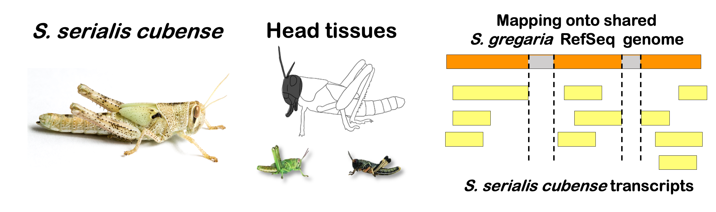
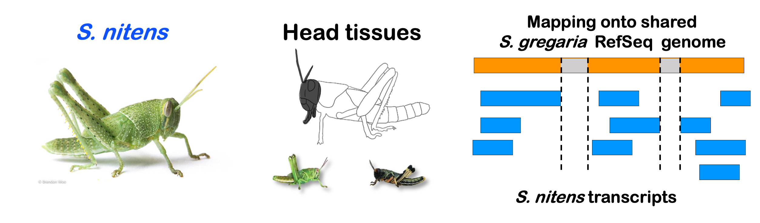
species_order <- c( "nitens", "cubense", "americana", "piceifrons", "cancellata", "gregaria")Here our objective is to compare the abundance, composition and
overlap of the DEGs found in the head and thorax tissues of each species
between the isolated and crowded last instar females. We found that the
differential genes expressed detected by DESeq2 varied
across species and tissues but we need some perspective: Are locusts
up-regulated and down-regulated the same genes? In the later section GO
enrichment, we will investigate what are the functions of these genes as
we will see that each species seems to show different gene expression
profiles in response to density changes.
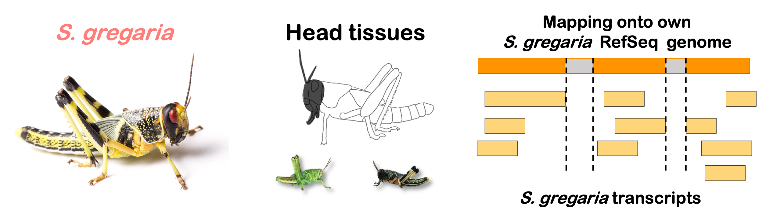
STRATEGY 1: One genome S. gregaria
1. DEGs comparison among species
We summarized the number of genes differential expressed between density for each species and each tissues.
# Initialize empty lists to store results
summary_list_head <- list()
summary_list_thorax <- list()

# Loop through each species to process their data
for (species in species_list) {
    # Read the DESeq2 results
  head_results_file <- file.path(workDir, "DEG_results/Bulk_RNAseq/", paste0(species, "/Head/DESeq2_results_Head_", species ,"_togregaria.csv"))
  thorax_results_file <- file.path(workDir, "DEG_results/Bulk_RNAseq/", paste0(species, "/Thorax/DESeq2_results_Thorax_", species ,"_togregaria.csv"))

    head_sigresults <- fread(head_results_file)  # fread is faster and uses less memory
    thorax_sigresults <- fread(thorax_results_file)

    # Count upregulated and downregulated genes for head
    head_upregulated <- sum(head_sigresults$log2FoldChange > 0)
    head_downregulated <- sum(head_sigresults$log2FoldChange < 0)
    head_upregulated_strict <- sum(head_sigresults$log2FoldChange > 1)
    head_downregulated_strict <- sum(head_sigresults$log2FoldChange < -1)

    # Count upregulated and downregulated genes for thorax
    thorax_upregulated <- sum(thorax_sigresults$log2FoldChange > 0)
    thorax_downregulated <- sum(thorax_sigresults$log2FoldChange < 0)
    thorax_upregulated_strict <- sum(thorax_sigresults$log2FoldChange > 1)
    thorax_downregulated_strict <- sum(thorax_sigresults$log2FoldChange < -1)

    # Store results in the list
    summary_list_head[[species]] <- data.frame(
        Species = species,
        Head_Upregulated = head_upregulated,
        Head_Downregulated = head_downregulated,
        Head_Upregulated_Strict = head_upregulated_strict,
        Head_Downregulated_Strict = head_downregulated_strict
    )

    summary_list_thorax[[species]] <- data.frame(
        Species = species,
        Thorax_Upregulated = thorax_upregulated,
        Thorax_Downregulated = thorax_downregulated,
        Thorax_Upregulated_Strict = thorax_upregulated_strict,
        Thorax_Downregulated_Strict = thorax_downregulated_strict
    )
}

# Combine lists into final data frames
summary_table_head <- bind_rows(summary_list_head)
summary_table_thorax <- bind_rows(summary_list_thorax)

# Print the summary table in a markdown-friendly format
knitr::kable(summary_table_head, format = "markdown", caption = "Summary of differentially expressed genes in head per species")| Species | Head_Upregulated | Head_Downregulated | Head_Upregulated_Strict | Head_Downregulated_Strict |
|---|---|---|---|---|
| gregaria | 2463 | 2529 | 458 | 364 |
| piceifrons | 381 | 383 | 185 | 183 |
| cancellata | 679 | 748 | 287 | 370 |
| americana | 689 | 501 | 299 | 245 |
| cubense | 26 | 26 | 26 | 26 |
| nitens | 189 | 269 | 102 | 213 |
# Convert the summary table to a long format for easier plotting
summary_long_head <- summary_table_head %>%
  pivot_longer(cols = c(Head_Upregulated_Strict, Head_Downregulated_Strict),
               names_to = "Tissue", values_to = "Count")

# Adjust the values for downregulated genes to be negative
summary_long_head <- summary_long_head %>%
  mutate(Count = ifelse(Tissue == "Head_Downregulated_Strict", -Count, Count))

summary_long_head$Species <- factor(summary_long_head$Species, levels = species_order)

# Plot barplot for head
ggplot(summary_long_head, aes(x = Species, y = Count, fill = Tissue)) +
  geom_bar(stat = "identity", position = "stack") +
  labs(title = "Upregulated and Downregulated Genes in Head (absolute lfc >1)",
       x = "Species", y = "Number of Genes") +
  scale_fill_manual(values = c("Head_Upregulated_Strict" = "red2", "Head_Downregulated_Strict" = "blue")) +
  scale_y_continuous(labels = function(x) ifelse(x < 0, -x, x), limits = c(-1200, 1200)) +
  theme_minimal(base_size = 12) +
  theme(legend.position = "top",
        plot.title = element_text(hjust = 0.5, size = 14, face = "bold"),
        axis.text.x = element_text(size = 12, angle = 45, hjust = 1)) +
  coord_flip()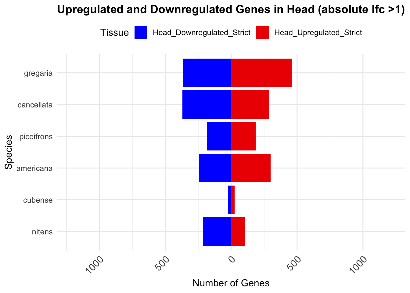
# Print the summary table for thorax
knitr::kable(summary_table_thorax, format = "markdown", caption = "Summary of differentially expressed genes in thorax per species")| Species | Thorax_Upregulated | Thorax_Downregulated | Thorax_Upregulated_Strict | Thorax_Downregulated_Strict |
|---|---|---|---|---|
| gregaria | 2194 | 2250 | 522 | 678 |
| piceifrons | 1579 | 1210 | 541 | 212 |
| cancellata | 697 | 628 | 286 | 297 |
| americana | 409 | 692 | 139 | 312 |
| cubense | 112 | 233 | 62 | 150 |
| nitens | 0 | 0 | 0 | 0 |
# Convert the summary table to a long format for thorax
summary_long_thorax <- summary_table_thorax %>%
  pivot_longer(cols = c(Thorax_Upregulated_Strict, Thorax_Downregulated_Strict),
               names_to = "Tissue", values_to = "Count")

# Adjust the values for downregulated genes to be negative
summary_long_thorax <- summary_long_thorax %>%
  mutate(Count = ifelse(Tissue == "Thorax_Downregulated_Strict", -Count, Count))

summary_long_thorax$Species <- factor(summary_long_thorax$Species, levels = species_order)

# Plot barplot for thorax
ggplot(summary_long_thorax, aes(x = Species, y = Count, fill = Tissue)) +
  geom_bar(stat = "identity", position = "stack") +
  labs(title = "Upregulated and Downregulated Genes in Thorax (absolute lfc >1)",
       x = "Species", y = "Number of Genes") +
  scale_fill_manual(values = c("Thorax_Upregulated_Strict" = "red2", "Thorax_Downregulated_Strict" = "blue")) +
  scale_y_continuous(labels = function(x) ifelse(x < 0, -x, x), limits = c(-1200, 1200)) +
  theme_minimal(base_size = 12) +
  theme(legend.position = "top",
        plot.title = element_text(hjust = 0.5, size = 14, face = "bold"),
        axis.text.x = element_text(size = 12, angle = 45, hjust = 1)) +
  coord_flip()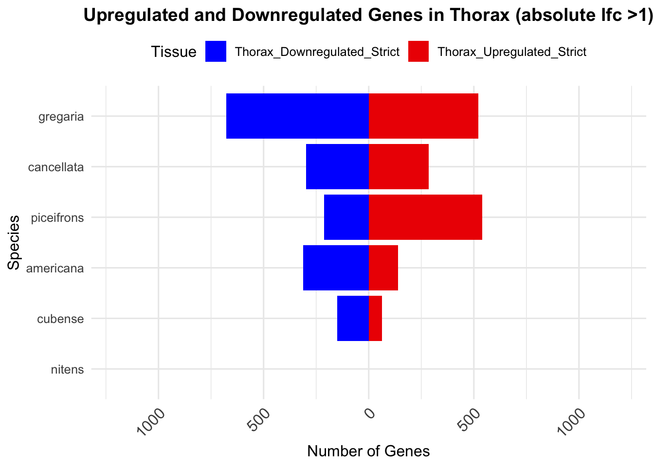
# Define custom colors for each GeneType
custom_colors <- c(
  "transcribed_pseudogene" = "#F4F1BB",  # Example color for transcribed_pseudogene
  "protein-coding" = "#9B57D3",         # Example color for protein-coding
  "lncRNA" = "#A5300F",                 # Example color for lncRNA
  "tRNA" = "#74D055FF",                   # Example color for tRNA
  "misc_RNA" = "#3B6978",               # Example color for misc_RNA
  "ncRNA" = "#29AF7FFF",                  # Example color for ncRNA
  "pseudogene" = "#81B29A",             # Example color for pseudogene
  "rRNA" = "#5982DB",                   # Example color for rRNA
  "snoRNA" = "#DCE318FF",                 # Example color for snoRNA
  "snRNA" = "#665EB8"                   # Example color for snRNA
)

# Use scale_fill_manual to map the custom colors to the GeneTypes
custom_color_scale <- scale_fill_manual(
  values = custom_colors
)
# Create an empty list to store the data for all species
all_species_data <- list()

# Loop through each species to process their data
for (species in species_list) {
  # Read the DESeq2 results for head and thorax
  head_results_file <- file.path(workDir, "DEG_results/Bulk_RNAseq/", paste0(species, "/Head/DESeq2_results_Head_", species ,"_togregaria.csv"))
  thorax_results_file <- file.path(workDir, "DEG_results/Bulk_RNAseq/", paste0(species, "/Thorax/DESeq2_results_Thorax_", species ,"_togregaria.csv"))

  head_sigresults <- read.csv(head_results_file, stringsAsFactors = FALSE)
  thorax_sigresults <- read.csv(thorax_results_file, stringsAsFactors = FALSE)

  # Add GeneType and Species columns (from `allspecies_df`)
  head_results_merged <- merge(head_sigresults, allspecies_df[, c("GeneID", "GeneType", "Species")], by = "GeneID")
  thorax_results_merged <- merge(thorax_sigresults, allspecies_df[, c("GeneID", "GeneType", "Species")], by = "GeneID")

  # Count for upregulated and downregulated genes in head
  head_upregulated <- head_results_merged %>%
    filter(log2FoldChange > 1) %>%
    mutate(Regulation = "Upregulated", Tissue = "Head", Count = 1)

  head_downregulated <- head_results_merged %>%
    filter(log2FoldChange < -1) %>%
    mutate(Regulation = "Downregulated", Tissue = "Head", Count = -1)  # Mutate downregulated genes to negative

  # Combine upregulated and downregulated genes for head
  head_combined <- rbind(head_upregulated, head_downregulated)

  # Ensure all GeneTypes are represented for this species, even if they have no DEGs
  head_combined <- head_combined %>%
    complete(GeneType = unique(allspecies_df$GeneType),
             fill = list(Count = 0))  # Fill missing GeneTypes with Count = 0

  # Count for upregulated and downregulated genes in thorax
  thorax_upregulated <- thorax_results_merged %>%
    filter(log2FoldChange > 1) %>%
    mutate(Regulation = "Upregulated", Tissue = "Thorax", Count = 1)

  thorax_downregulated <- thorax_results_merged %>%
    filter(log2FoldChange < -1) %>%
    mutate(Regulation = "Downregulated", Tissue = "Thorax", Count = -1)  # Mutate downregulated genes to negative

  # Combine upregulated and downregulated genes for thorax
  thorax_combined <- rbind(thorax_upregulated, thorax_downregulated)

  # Ensure all GeneTypes are represented for this species in thorax, even if they have no DEGs
  thorax_combined <- thorax_combined %>%
    complete(GeneType = unique(allspecies_df$GeneType),
             fill = list(Count = 0))  # Fill missing GeneTypes with Count = 0

  # Combine data for head and thorax into one
  combined_data <- rbind(head_combined, thorax_combined)

  # Add species column to the data
  combined_data$Species <- species

  # Append the data to the list for all species
  all_species_data[[species]] <- combined_data
}

# Combine all species data into one data frame
final_data <- bind_rows(all_species_data)

# Reorder species according to the desired order
final_data$Species <- factor(final_data$Species, levels = species_order)

# Filter for head tissue only
final_data_head <- final_data %>% filter(Tissue == "Head")
final_data_thorax <- final_data %>% filter(Tissue == "Thorax")

# Create the barplot for all species and only head tissue
ggplot(final_data_head, aes(x = Species, y = Count, fill = GeneType)) +
  geom_bar(stat = "identity", position = "stack") +
  labs(title = "DEGs by Gene Biotype for Head (absolute lfc >1)",
       x = "Species",
       y = "Number of Genes") +
  custom_color_scale +
  scale_y_continuous(labels = function(x) ifelse(x < 0, -x, x), limits = c(-1200, 1200))+
theme_minimal(base_size = 12) +
  theme(legend.position = "top",
        plot.title = element_text(hjust = 0.5, size = 14, face = "bold"),
        axis.title.x = element_text(size = 14, face = "bold"),
        axis.title.y = element_text(size = 14, face = "bold"),
        axis.text.x = element_text(size = 12, angle = 45, hjust = 1),
        axis.text.y = element_text(size = 12),
        panel.grid.major.y = element_line(color = "grey90", linetype = "dashed"),
        panel.grid.minor = element_blank()) +
  coord_flip()  # Flip coordinates to make the plot horizontal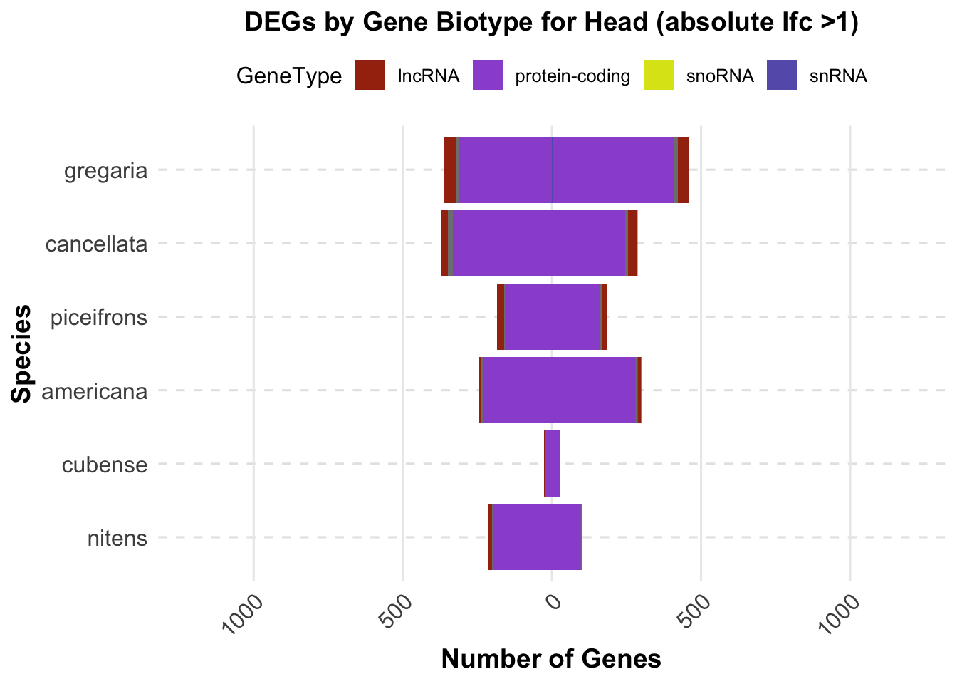
# Create the barplot for all species and only head tissue
ggplot(final_data_thorax, aes(x = Species, y = Count, fill = GeneType)) +
  geom_bar(stat = "identity", position = "stack") +
  labs(title = "DEGs by Gene Biotype for Thorax (absolute lfc >1)",
       x = "Species",
       y = "Number of Genes") +
  custom_color_scale +
  scale_y_continuous(labels = function(x) ifelse(x < 0, -x, x), limits = c(-1200, 1200))+
theme_minimal(base_size = 12) +
  theme(legend.position = "top",
        plot.title = element_text(hjust = 0.5, size = 14, face = "bold"),
        axis.title.x = element_text(size = 14, face = "bold"),
        axis.title.y = element_text(size = 14, face = "bold"),
        axis.text.x = element_text(size = 12, angle = 45, hjust = 1),
        axis.text.y = element_text(size = 12),
        panel.grid.major.y = element_line(color = "grey90", linetype = "dashed"),
        panel.grid.minor = element_blank()) +
  coord_flip()  # Flip coordinates to make the plot horizontal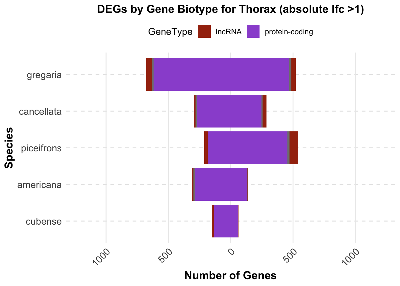
2. Overlap DEGs between tissues
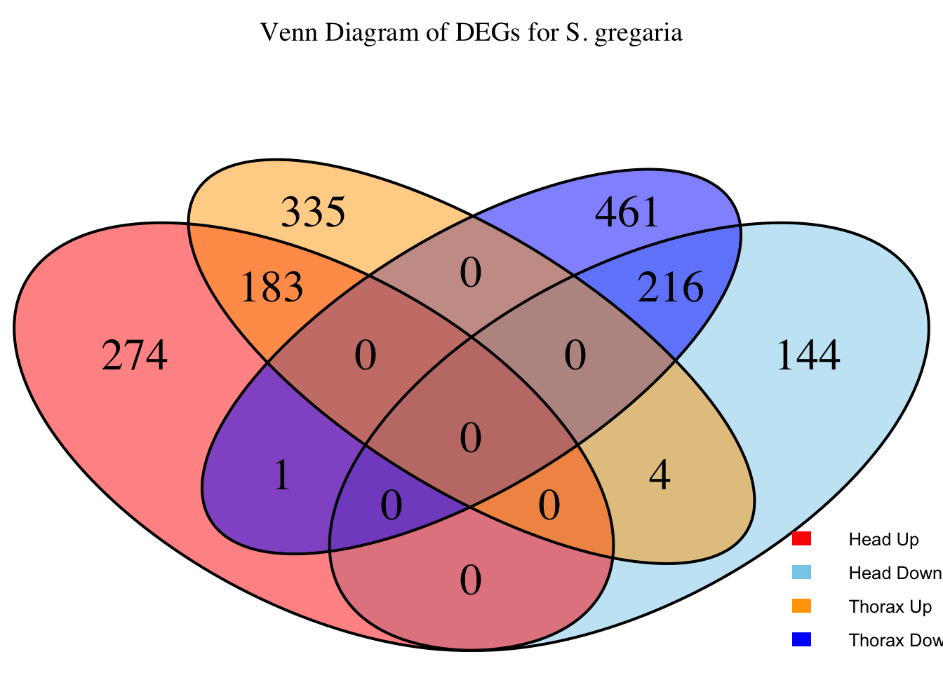
gregaria
species <- "gregaria"  # Specify the species for which to generate plots

# Load DESeq2 results for head and thorax
head_file <- file.path(workDir, "DEG_results/Bulk_RNAseq/", paste0(species, "/Head/DESeq2_results_Head_", species,"_togregaria.csv"))
thorax_file <- file.path(workDir, "DEG_results/Bulk_RNAseq/", paste0(species, "/Thorax/DESeq2_results_Thorax_", species,"_togregaria.csv"))


head_data <- read.csv(head_file, stringsAsFactors = FALSE)
thorax_data <- read.csv(thorax_file, stringsAsFactors = FALSE)

# Check if data is empty and handle accordingly
if (nrow(head_data) == 0 || nrow(thorax_data) == 0) {
    message(paste("No data for species:", species))
} else {
    # Filter for significant DEGs and select upregulated and downregulated genes
    head_up <- head_data %>%
        filter(padj < 0.05 & log2FoldChange > 1) %>%
        select(GeneID = X)

    head_down <- head_data %>%
        filter(padj < 0.05 & log2FoldChange < -1) %>%
        select(GeneID = X)

    thorax_up <- thorax_data %>%
        filter(padj < 0.05 & log2FoldChange > 1) %>%
        select(GeneID = X)

    thorax_down <- thorax_data %>%
        filter(padj < 0.05 & log2FoldChange < -1) %>%
        select(GeneID = X)

    # Prepare data for Venn diagram
    venn_data <- list(
        Head_Upregulated = head_up$GeneID,
        Head_Downregulated = head_down$GeneID,
        Thorax_Upregulated = thorax_up$GeneID,
        Thorax_Downregulated = thorax_down$GeneID
    )

    # Generate the four-way Venn diagram with specified colors and legend outside
    venn_plot <- venn.diagram(
        x = venn_data,
        category.names = c("Head Upregulated", "Head Downregulated", "Thorax Upregulated", "Thorax Downregulated"),
        filename = NULL,
        output = TRUE,
        fill = c("red", "skyblue", "orange", "blue"),  # Set colors for upregulated and downregulated
        alpha = 0.5,
        cex = 2,  # Text size for numbers
        cat.cex = 0,  # Text size for category labels
        cat.pos = c(0, 0, 0, 0),  # Position to center labels
        cat.dist = c(0.1, 0.1, 0.1, 0.1),  # Distance between category labels and circles
        main = paste("Venn Diagram of DEGs for S.", species),
        main.cex = 1.2,  # Size of the main title
        cat.col = c("red", "skyblue", "orange", "blue")  # Color the category labels
    )

    # Clear the current plotting area before drawing the next Venn diagram
    grid.newpage()

    # Display the Venn diagram
    grid.draw(venn_plot)

    # Manually create a custom legend
    legend_labels <- c("Head Up", "Head Down", "Thorax Up", "Thorax Down")
    legend_colors <- c("red", "skyblue", "orange", "blue")

    # Positioning the legend lower on the right side of the plot
    legend_x <- unit(0.85, "npc")  # Adjust x position
    legend_y <- unit(0.2, "npc")    # Lower the legend vertically

    # Draw the legend
    for (i in 1:length(legend_labels)) {
        grid.rect(x = legend_x, y = legend_y - unit((i - 1) * 0.05, "npc"),
                  width = unit(0.02, "npc"), height = unit(0.02, "npc"),
                  gp = gpar(fill = legend_colors[i], col = NA))
        grid.text(label = legend_labels[i], x = legend_x + unit(0.05, "npc"),
                  y = legend_y - unit((i - 1) * 0.05, "npc"),
                  just = "left", gp = gpar(cex = 0.8))
    }

    # Scatter plot for overlapping genes
    # Filter significant DEGs for both head and thorax
    head_sig_genes <- head_data %>%
        filter(padj < 0.05 & abs(log2FoldChange) > 1) %>%
        select(GeneID = X, log2FoldChange, padj)

    thorax_sig_genes <- thorax_data %>%
        filter(padj < 0.05 & abs(log2FoldChange) > 1) %>%
        select(GeneID = X, log2FoldChange, padj)

    # Find overlapping genes based on GeneID
    overlapping_genes <- inner_join(head_sig_genes, thorax_sig_genes, by = "GeneID", suffix = c("_head", "_thorax"))

    # Save the overlapping genes to a CSV file
    output_file <- file.path(workDir, "overlap/Bulk_RNAseq", paste0("overlapping_genes_head_thorax_", species, ".csv"))
    write.csv(overlapping_genes, output_file, row.names = FALSE)

    # Plot overlapping genes with scatter plot
    p <- ggplot(overlapping_genes, aes(x = log2FoldChange_head, y = log2FoldChange_thorax)) +
        geom_point(aes(color = case_when(
            log2FoldChange_head > 0 & log2FoldChange_thorax > 0 ~ "Upregulated in Both",
            log2FoldChange_head < 0 & log2FoldChange_thorax < 0 ~ "Downregulated in Both",
            log2FoldChange_head > 0 & log2FoldChange_thorax < 0 ~ "Up in Head, Down in Thorax",
            log2FoldChange_head < 0 & log2FoldChange_thorax > 0 ~ "Down in Head, Up in Thorax"
        )), size = 3, alpha = 0.7) +
        geom_abline(slope = 1, intercept = 0, linetype = "dashed", color = "gray") +
        labs(
            x = "Log2 Fold Change (Head)",
            y = "Log2 Fold Change (Thorax)",
            color = "Regulation Pattern",
            title = "Comparison of Log2 Fold Changes in Overlapping Genes",
            subtitle = paste("Head vs. Thorax in", species)
        ) +
        theme_minimal() +
        theme(
            plot.title = element_text(size = 16, face = "bold"),
            plot.subtitle = element_text(size = 12, face = "italic"),
            legend.position = "top"
        ) +
        scale_color_manual(values = c(
            "Upregulated in Both" = "red",
            "Downregulated in Both" = "blue",
            "Up in Head, Down in Thorax" = "purple",
            "Down in Head, Up in Thorax" = "green"
        ))

    # Save the scatter plot
    ggsave(filename = file.path(workDir, "overlap/Bulk_RNAseq", paste0("scatter_plot_overlapping_genes_", species, ".png")), plot = p)

    # Display the scatter plot
    print(p)
}

piceifrons
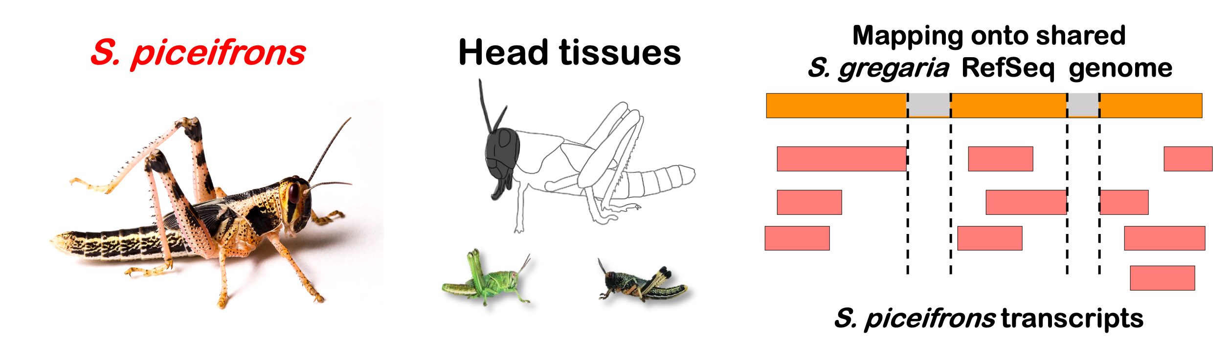
species <- "piceifrons" # Specify the species for which to generate plots
# Load DESeq2 results for head and thorax
head_file <- file.path(workDir, "DEG_results/Bulk_RNAseq/", paste0(species, "/Head/DESeq2_results_Head_", species,"_togregaria.csv"))
thorax_file <- file.path(workDir, "DEG_results/Bulk_RNAseq/", paste0(species, "/Thorax/DESeq2_results_Thorax_", species,"_togregaria.csv"))
head_data <- read.csv(head_file, stringsAsFactors = FALSE)
thorax_data <- read.csv(thorax_file, stringsAsFactors = FALSE)
# Check if data is empty and handle accordingly
if (nrow(head_data) == 0 || nrow(thorax_data) == 0) {
message(paste("No data for species:", species))
} else {
# Filter for significant DEGs and select upregulated and downregulated genes
head_up <- head_data %>%
filter(padj < 0.05 & log2FoldChange > 1) %>%
select(GeneID = X)
head_down <- head_data %>%
filter(padj < 0.05 & log2FoldChange < -1) %>%
select(GeneID = X)
thorax_up <- thorax_data %>%
filter(padj < 0.05 & log2FoldChange > 1) %>%
select(GeneID = X)
thorax_down <- thorax_data %>%
filter(padj < 0.05 & log2FoldChange < -1) %>%
select(GeneID = X)
# Prepare data for Venn diagram
venn_data <- list(
Head_Upregulated = head_up$GeneID,
Head_Downregulated = head_down$GeneID,
Thorax_Upregulated = thorax_up$GeneID,
Thorax_Downregulated = thorax_down$GeneID
)
# Generate the four-way Venn diagram with specified colors and legend outside
venn_plot <- venn.diagram(
x = venn_data,
category.names = c("Head Upregulated", "Head Downregulated", "Thorax Upregulated", "Thorax Downregulated"),
filename = NULL,
output = TRUE,
fill = c("red", "skyblue", "orange", "blue"), # Set colors for upregulated and downregulated
alpha = 0.5,
cex = 2, # Text size for numbers
cat.cex = 0, # Text size for category labels
cat.pos = c(0, 0, 0, 0), # Position to center labels
cat.dist = c(0.1, 0.1, 0.1, 0.1), # Distance between category labels and circles
main = paste("Venn Diagram of DEGs for S.", species),
main.cex = 1.2, # Size of the main title
cat.col = c("red", "skyblue", "orange", "blue") # Color the category labels
)
# Clear the current plotting area before drawing the next Venn diagram
grid.newpage()
# Display the Venn diagram
grid.draw(venn_plot)
# Manually create a custom legend
legend_labels <- c("Head Up", "Head Down", "Thorax Up", "Thorax Down")
legend_colors <- c("red", "skyblue", "orange", "blue")
# Positioning the legend lower on the right side of the plot
legend_x <- unit(0.85, "npc") # Adjust x position
legend_y <- unit(0.2, "npc") # Lower the legend vertically
# Draw the legend
for (i in 1:length(legend_labels)) {
grid.rect(x = legend_x, y = legend_y - unit((i - 1) * 0.05, "npc"),
width = unit(0.02, "npc"), height = unit(0.02, "npc"),
gp = gpar(fill = legend_colors[i], col = NA))
grid.text(label = legend_labels[i], x = legend_x + unit(0.05, "npc"),
y = legend_y - unit((i - 1) * 0.05, "npc"),
just = "left", gp = gpar(cex = 0.8))
}
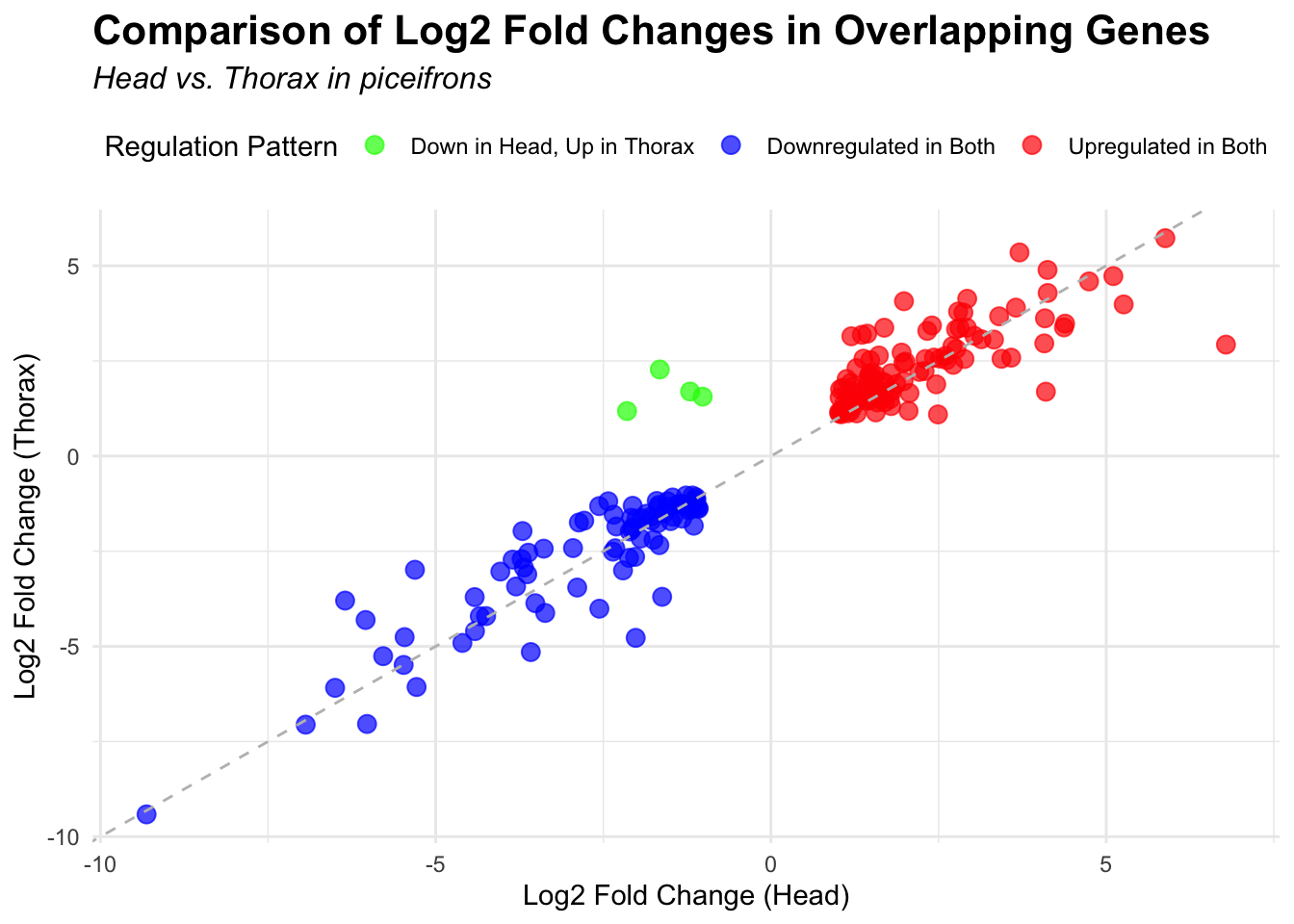
# Scatter plot for overlapping genes
# Filter significant DEGs for both head and thorax
head_sig_genes <- head_data %>%
filter(padj < 0.05 & abs(log2FoldChange) > 1) %>%
select(GeneID = X, log2FoldChange, padj)
thorax_sig_genes <- thorax_data %>%
filter(padj < 0.05 & abs(log2FoldChange) > 1) %>%
select(GeneID = X, log2FoldChange, padj)
# Find overlapping genes based on GeneID
overlapping_genes <- inner_join(head_sig_genes, thorax_sig_genes, by = "GeneID", suffix = c("_head", "_thorax"))
# Save the overlapping genes to a CSV file
output_file <- file.path(workDir, "overlap/Bulk_RNAseq", paste0("overlapping_genes_head_thorax_", species, ".csv"))
write.csv(overlapping_genes, output_file, row.names = FALSE)
# Plot overlapping genes with scatter plot
p <- ggplot(overlapping_genes, aes(x = log2FoldChange_head, y = log2FoldChange_thorax)) +
geom_point(aes(color = case_when(
log2FoldChange_head > 0 & log2FoldChange_thorax > 0 ~ "Upregulated in Both",
log2FoldChange_head < 0 & log2FoldChange_thorax < 0 ~ "Downregulated in Both",
log2FoldChange_head > 0 & log2FoldChange_thorax < 0 ~ "Up in Head, Down in Thorax",
log2FoldChange_head < 0 & log2FoldChange_thorax > 0 ~ "Down in Head, Up in Thorax"
)), size = 3, alpha = 0.7) +
geom_abline(slope = 1, intercept = 0, linetype = "dashed", color = "gray") +
labs(
x = "Log2 Fold Change (Head)",
y = "Log2 Fold Change (Thorax)",
color = "Regulation Pattern",
title = "Comparison of Log2 Fold Changes in Overlapping Genes",
subtitle = paste("Head vs. Thorax in", species)
) +
theme_minimal() +
theme(
plot.title = element_text(size = 16, face = "bold"),
plot.subtitle = element_text(size = 12, face = "italic"),
legend.position = "top"
) +
scale_color_manual(values = c(
"Upregulated in Both" = "red",
"Downregulated in Both" = "blue",
"Up in Head, Down in Thorax" = "purple",
"Down in Head, Up in Thorax" = "green"
))
# Save the scatter plot
ggsave(filename = file.path(workDir, "overlap/Bulk_RNAseq", paste0("scatter_plot_overlapping_genes_", species, ".png")), plot = p)
# Display the scatter plot
print(p)
}
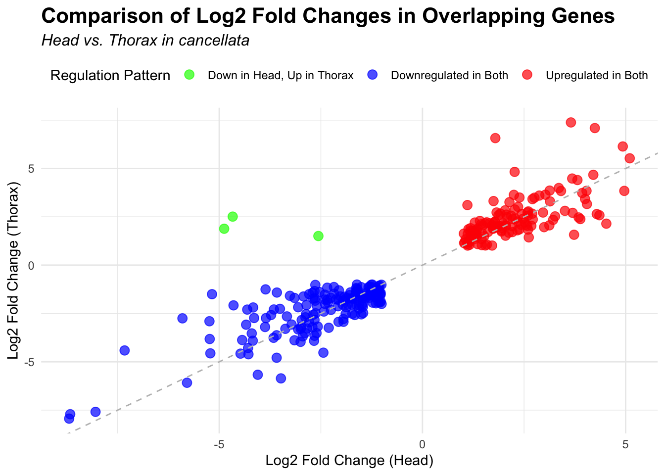
cancellata
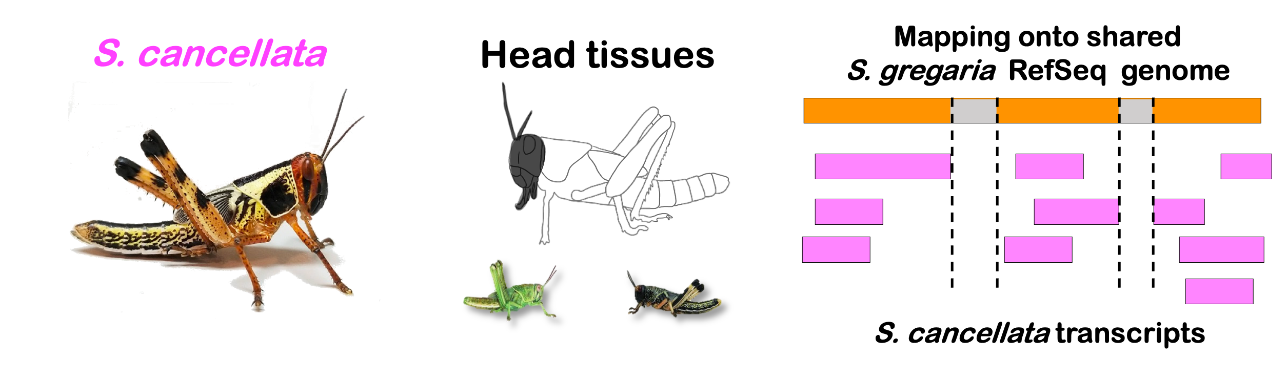
species <- "cancellata"  # Specify the species for which to generate plots

# Load DESeq2 results for head and thorax
head_file <- file.path(workDir, "DEG_results/Bulk_RNAseq/", paste0(species, "/Head/DESeq2_results_Head_", species,"_togregaria.csv"))
thorax_file <- file.path(workDir, "DEG_results/Bulk_RNAseq/", paste0(species, "/Thorax/DESeq2_results_Thorax_", species,"_togregaria.csv"))

head_data <- read.csv(head_file, stringsAsFactors = FALSE)
thorax_data <- read.csv(thorax_file, stringsAsFactors = FALSE)

# Check if data is empty and handle accordingly
if (nrow(head_data) == 0 || nrow(thorax_data) == 0) {
    message(paste("No data for species:", species))
} else {
    # Filter for significant DEGs and select upregulated and downregulated genes
    head_up <- head_data %>%
        filter(padj < 0.05 & log2FoldChange > 1) %>%
        select(GeneID = X)

    head_down <- head_data %>%
        filter(padj < 0.05 & log2FoldChange < -1) %>%
        select(GeneID = X)

    thorax_up <- thorax_data %>%
        filter(padj < 0.05 & log2FoldChange > 1) %>%
        select(GeneID = X)

    thorax_down <- thorax_data %>%
        filter(padj < 0.05 & log2FoldChange < -1) %>%
        select(GeneID = X)

    # Prepare data for Venn diagram
    venn_data <- list(
        Head_Upregulated = head_up$GeneID,
        Head_Downregulated = head_down$GeneID,
        Thorax_Upregulated = thorax_up$GeneID,
        Thorax_Downregulated = thorax_down$GeneID
    )

    # Generate the four-way Venn diagram with specified colors and legend outside
    venn_plot <- venn.diagram(
        x = venn_data,
        category.names = c("Head Upregulated", "Head Downregulated", "Thorax Upregulated", "Thorax Downregulated"),
        filename = NULL,
        output = TRUE,
        fill = c("red", "skyblue", "orange", "blue"),  # Set colors for upregulated and downregulated
        alpha = 0.5,
        cex = 2,  # Text size for numbers
        cat.cex = 0,  # Text size for category labels
        cat.pos = c(0, 0, 0, 0),  # Position to center labels
        cat.dist = c(0.1, 0.1, 0.1, 0.1),  # Distance between category labels and circles
        main = paste("Venn Diagram of DEGs for S.", species),
        main.cex = 1.2,  # Size of the main title
        cat.col = c("red", "skyblue", "orange", "blue")  # Color the category labels
    )

    # Clear the current plotting area before drawing the next Venn diagram
    grid.newpage()

    # Display the Venn diagram
    grid.draw(venn_plot)

    # Manually create a custom legend
    legend_labels <- c("Head Up", "Head Down", "Thorax Up", "Thorax Down")
    legend_colors <- c("red", "skyblue", "orange", "blue")

    # Positioning the legend lower on the right side of the plot
    legend_x <- unit(0.85, "npc")  # Adjust x position
    legend_y <- unit(0.2, "npc")    # Lower the legend vertically

    # Draw the legend
    for (i in 1:length(legend_labels)) {
        grid.rect(x = legend_x, y = legend_y - unit((i - 1) * 0.05, "npc"),
                  width = unit(0.02, "npc"), height = unit(0.02, "npc"),
                  gp = gpar(fill = legend_colors[i], col = NA))
        grid.text(label = legend_labels[i], x = legend_x + unit(0.05, "npc"),
                  y = legend_y - unit((i - 1) * 0.05, "npc"),
                  just = "left", gp = gpar(cex = 0.8))
    }

    # Scatter plot for overlapping genes
    # Filter significant DEGs for both head and thorax
    head_sig_genes <- head_data %>%
        filter(padj < 0.05 & abs(log2FoldChange) > 1) %>%
        select(GeneID = X, log2FoldChange, padj)

    thorax_sig_genes <- thorax_data %>%
        filter(padj < 0.05 & abs(log2FoldChange) > 1) %>%
        select(GeneID = X, log2FoldChange, padj)

    # Find overlapping genes based on GeneID
    overlapping_genes <- inner_join(head_sig_genes, thorax_sig_genes, by = "GeneID", suffix = c("_head", "_thorax"))

    # Save the overlapping genes to a CSV file
    output_file <- file.path(workDir, "overlap/Bulk_RNAseq", paste0("overlapping_genes_head_thorax_", species, ".csv"))
    write.csv(overlapping_genes, output_file, row.names = FALSE)

    # Plot overlapping genes with scatter plot
    p <- ggplot(overlapping_genes, aes(x = log2FoldChange_head, y = log2FoldChange_thorax)) +
        geom_point(aes(color = case_when(
            log2FoldChange_head > 0 & log2FoldChange_thorax > 0 ~ "Upregulated in Both",
            log2FoldChange_head < 0 & log2FoldChange_thorax < 0 ~ "Downregulated in Both",
            log2FoldChange_head > 0 & log2FoldChange_thorax < 0 ~ "Up in Head, Down in Thorax",
            log2FoldChange_head < 0 & log2FoldChange_thorax > 0 ~ "Down in Head, Up in Thorax"
        )), size = 3, alpha = 0.7) +
        geom_abline(slope = 1, intercept = 0, linetype = "dashed", color = "gray") +
        labs(
            x = "Log2 Fold Change (Head)",
            y = "Log2 Fold Change (Thorax)",
            color = "Regulation Pattern",
            title = "Comparison of Log2 Fold Changes in Overlapping Genes",
            subtitle = paste("Head vs. Thorax in", species)
        ) +
        theme_minimal() +
        theme(
            plot.title = element_text(size = 16, face = "bold"),
            plot.subtitle = element_text(size = 12, face = "italic"),
            legend.position = "top"
        ) +
        scale_color_manual(values = c(
            "Upregulated in Both" = "red",
            "Downregulated in Both" = "blue",
            "Up in Head, Down in Thorax" = "purple",
            "Down in Head, Up in Thorax" = "green"
        ))

    # Save the scatter plot
    ggsave(filename = file.path(workDir, "overlap/Bulk_RNAseq", paste0("scatter_plot_overlapping_genes_", species, ".png")), plot = p)

    # Display the scatter plot
    print(p)
}
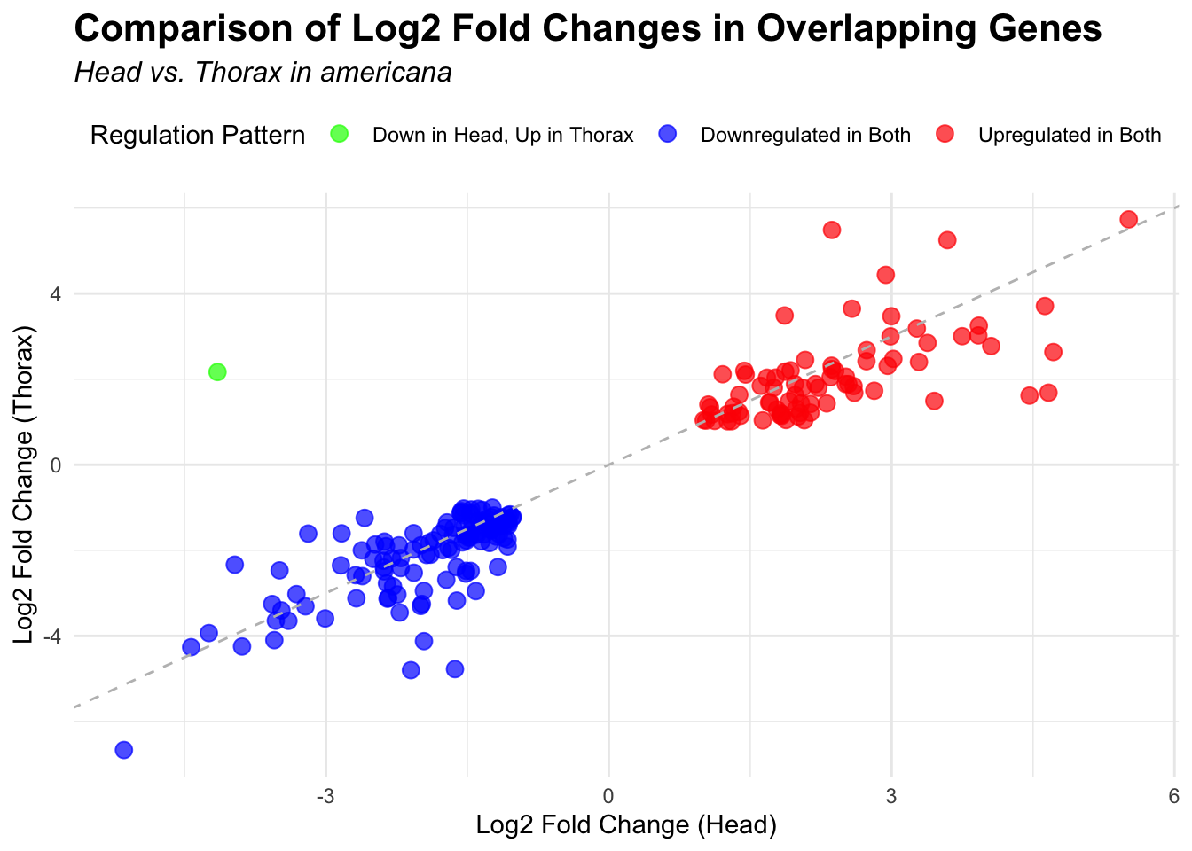
americana
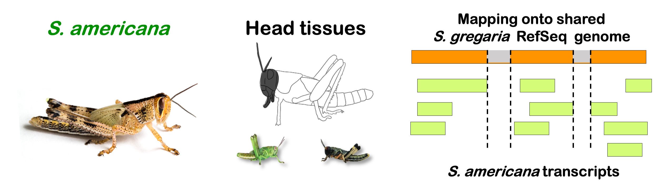
species <- "americana"  # Specify the species for which to generate plots

# Load DESeq2 results for head and thorax
head_file <- file.path(workDir, "DEG_results/Bulk_RNAseq/", paste0(species, "/Head/DESeq2_results_Head_", species,"_togregaria.csv"))
thorax_file <- file.path(workDir, "DEG_results/Bulk_RNAseq/", paste0(species, "/Thorax/DESeq2_results_Thorax_", species,"_togregaria.csv"))

head_data <- read.csv(head_file, stringsAsFactors = FALSE)
thorax_data <- read.csv(thorax_file, stringsAsFactors = FALSE)

# Check if data is empty and handle accordingly
if (nrow(head_data) == 0 || nrow(thorax_data) == 0) {
    message(paste("No data for species:", species))
} else {
    # Filter for significant DEGs and select upregulated and downregulated genes
    head_up <- head_data %>%
        filter(padj < 0.05 & log2FoldChange > 1) %>%
        select(GeneID = X)

    head_down <- head_data %>%
        filter(padj < 0.05 & log2FoldChange < -1) %>%
        select(GeneID = X)

    thorax_up <- thorax_data %>%
        filter(padj < 0.05 & log2FoldChange > 1) %>%
        select(GeneID = X)

    thorax_down <- thorax_data %>%
        filter(padj < 0.05 & log2FoldChange < -1) %>%
        select(GeneID = X)

    # Prepare data for Venn diagram
    venn_data <- list(
        Head_Upregulated = head_up$GeneID,
        Head_Downregulated = head_down$GeneID,
        Thorax_Upregulated = thorax_up$GeneID,
        Thorax_Downregulated = thorax_down$GeneID
    )

    # Generate the four-way Venn diagram with specified colors and legend outside
    venn_plot <- venn.diagram(
        x = venn_data,
        category.names = c("Head Upregulated", "Head Downregulated", "Thorax Upregulated", "Thorax Downregulated"),
        filename = NULL,
        output = TRUE,
        fill = c("red", "skyblue", "orange", "blue"),  # Set colors for upregulated and downregulated
        alpha = 0.5,
        cex = 2,  # Text size for numbers
        cat.cex = 0,  # Text size for category labels
        cat.pos = c(0, 0, 0, 0),  # Position to center labels
        cat.dist = c(0.1, 0.1, 0.1, 0.1),  # Distance between category labels and circles
        main = paste("Venn Diagram of DEGs for S.", species),
        main.cex = 1.2,  # Size of the main title
        cat.col = c("red", "skyblue", "orange", "blue")  # Color the category labels
    )

    # Clear the current plotting area before drawing the next Venn diagram
    grid.newpage()

    # Display the Venn diagram
    grid.draw(venn_plot)

    # Manually create a custom legend
    legend_labels <- c("Head Up", "Head Down", "Thorax Up", "Thorax Down")
    legend_colors <- c("red", "skyblue", "orange", "blue")

    # Positioning the legend lower on the right side of the plot
    legend_x <- unit(0.85, "npc")  # Adjust x position
    legend_y <- unit(0.2, "npc")    # Lower the legend vertically

    # Draw the legend
    for (i in 1:length(legend_labels)) {
        grid.rect(x = legend_x, y = legend_y - unit((i - 1) * 0.05, "npc"),
                  width = unit(0.02, "npc"), height = unit(0.02, "npc"),
                  gp = gpar(fill = legend_colors[i], col = NA))
        grid.text(label = legend_labels[i], x = legend_x + unit(0.05, "npc"),
                  y = legend_y - unit((i - 1) * 0.05, "npc"),
                  just = "left", gp = gpar(cex = 0.8))
    }

    # Scatter plot for overlapping genes
    # Filter significant DEGs for both head and thorax
    head_sig_genes <- head_data %>%
        filter(padj < 0.05 & abs(log2FoldChange) > 1) %>%
        select(GeneID = X, log2FoldChange, padj)

    thorax_sig_genes <- thorax_data %>%
        filter(padj < 0.05 & abs(log2FoldChange) > 1) %>%
        select(GeneID = X, log2FoldChange, padj)

    # Find overlapping genes based on GeneID
    overlapping_genes <- inner_join(head_sig_genes, thorax_sig_genes, by = "GeneID", suffix = c("_head", "_thorax"))

    # Save the overlapping genes to a CSV file
    output_file <- file.path(workDir, "overlap/Bulk_RNAseq", paste0("overlapping_genes_head_thorax_", species, ".csv"))
    write.csv(overlapping_genes, output_file, row.names = FALSE)

    # Plot overlapping genes with scatter plot
    p <- ggplot(overlapping_genes, aes(x = log2FoldChange_head, y = log2FoldChange_thorax)) +
        geom_point(aes(color = case_when(
            log2FoldChange_head > 0 & log2FoldChange_thorax > 0 ~ "Upregulated in Both",
            log2FoldChange_head < 0 & log2FoldChange_thorax < 0 ~ "Downregulated in Both",
            log2FoldChange_head > 0 & log2FoldChange_thorax < 0 ~ "Up in Head, Down in Thorax",
            log2FoldChange_head < 0 & log2FoldChange_thorax > 0 ~ "Down in Head, Up in Thorax"
        )), size = 3, alpha = 0.7) +
        geom_abline(slope = 1, intercept = 0, linetype = "dashed", color = "gray") +
        labs(
            x = "Log2 Fold Change (Head)",
            y = "Log2 Fold Change (Thorax)",
            color = "Regulation Pattern",
            title = "Comparison of Log2 Fold Changes in Overlapping Genes",
            subtitle = paste("Head vs. Thorax in", species)
        ) +
        theme_minimal() +
        theme(
            plot.title = element_text(size = 16, face = "bold"),
            plot.subtitle = element_text(size = 12, face = "italic"),
            legend.position = "top"
        ) +
        scale_color_manual(values = c(
            "Upregulated in Both" = "red",
            "Downregulated in Both" = "blue",
            "Up in Head, Down in Thorax" = "purple",
            "Down in Head, Up in Thorax" = "green"
        ))

    # Save the scatter plot
    ggsave(filename = file.path(workDir, "overlap/Bulk_RNAseq", paste0("scatter_plot_overlapping_genes_", species, ".png")), plot = p)

    # Display the scatter plot
    print(p)
}
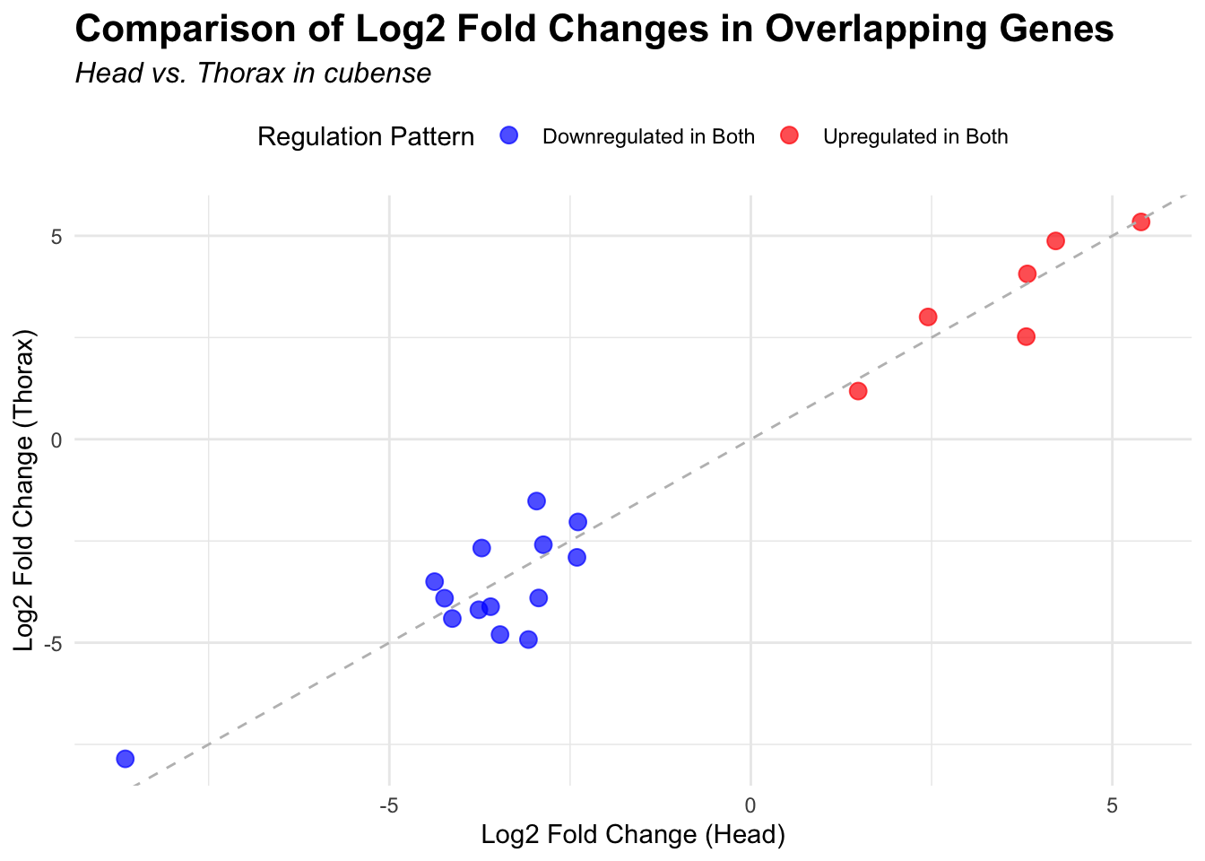
cubense
species <- "cubense"  # Specify the species for which to generate plots

# Load DESeq2 results for head and thorax
head_file <- file.path(workDir, "DEG_results/Bulk_RNAseq/", paste0(species, "/Head/DESeq2_results_Head_", species,"_togregaria.csv"))
thorax_file <- file.path(workDir, "DEG_results/Bulk_RNAseq/", paste0(species, "/Thorax/DESeq2_results_Thorax_", species,"_togregaria.csv"))

head_data <- read.csv(head_file, stringsAsFactors = FALSE)
thorax_data <- read.csv(thorax_file, stringsAsFactors = FALSE)

# Check if data is empty and handle accordingly
if (nrow(head_data) == 0 || nrow(thorax_data) == 0) {
    message(paste("No data for species:", species))
} else {
    # Filter for significant DEGs and select upregulated and downregulated genes
    head_up <- head_data %>%
        filter(padj < 0.05 & log2FoldChange > 1) %>%
        select(GeneID = X)

    head_down <- head_data %>%
        filter(padj < 0.05 & log2FoldChange < -1) %>%
        select(GeneID = X)

    thorax_up <- thorax_data %>%
        filter(padj < 0.05 & log2FoldChange > 1) %>%
        select(GeneID = X)

    thorax_down <- thorax_data %>%
        filter(padj < 0.05 & log2FoldChange < -1) %>%
        select(GeneID = X)

    # Prepare data for Venn diagram
    venn_data <- list(
        Head_Upregulated = head_up$GeneID,
        Head_Downregulated = head_down$GeneID,
        Thorax_Upregulated = thorax_up$GeneID,
        Thorax_Downregulated = thorax_down$GeneID
    )

    # Generate the four-way Venn diagram with specified colors and legend outside
    venn_plot <- venn.diagram(
        x = venn_data,
        category.names = c("Head Upregulated", "Head Downregulated", "Thorax Upregulated", "Thorax Downregulated"),
        filename = NULL,
        output = TRUE,
        fill = c("red", "skyblue", "orange", "blue"),  # Set colors for upregulated and downregulated
        alpha = 0.5,
        cex = 2,  # Text size for numbers
        cat.cex = 0,  # Text size for category labels
        cat.pos = c(0, 0, 0, 0),  # Position to center labels
        cat.dist = c(0.1, 0.1, 0.1, 0.1),  # Distance between category labels and circles
        main = paste("Venn Diagram of DEGs for S.", species),
        main.cex = 1.2,  # Size of the main title
        cat.col = c("red", "skyblue", "orange", "blue")  # Color the category labels
    )

    # Clear the current plotting area before drawing the next Venn diagram
    grid.newpage()

    # Display the Venn diagram
    grid.draw(venn_plot)

    # Manually create a custom legend
    legend_labels <- c("Head Up", "Head Down", "Thorax Up", "Thorax Down")
    legend_colors <- c("red", "skyblue", "orange", "blue")

    # Positioning the legend lower on the right side of the plot
    legend_x <- unit(0.85, "npc")  # Adjust x position
    legend_y <- unit(0.2, "npc")    # Lower the legend vertically

    # Draw the legend
    for (i in 1:length(legend_labels)) {
        grid.rect(x = legend_x, y = legend_y - unit((i - 1) * 0.05, "npc"),
                  width = unit(0.02, "npc"), height = unit(0.02, "npc"),
                  gp = gpar(fill = legend_colors[i], col = NA))
        grid.text(label = legend_labels[i], x = legend_x + unit(0.05, "npc"),
                  y = legend_y - unit((i - 1) * 0.05, "npc"),
                  just = "left", gp = gpar(cex = 0.8))
    }

    # Scatter plot for overlapping genes
    # Filter significant DEGs for both head and thorax
    head_sig_genes <- head_data %>%
        filter(padj < 0.05 & abs(log2FoldChange) > 1) %>%
        select(GeneID = X, log2FoldChange, padj)

    thorax_sig_genes <- thorax_data %>%
        filter(padj < 0.05 & abs(log2FoldChange) > 1) %>%
        select(GeneID = X, log2FoldChange, padj)

    # Find overlapping genes based on GeneID
    overlapping_genes <- inner_join(head_sig_genes, thorax_sig_genes, by = "GeneID", suffix = c("_head", "_thorax"))

    # Save the overlapping genes to a CSV file
    output_file <- file.path(workDir, "overlap/Bulk_RNAseq", paste0("overlapping_genes_head_thorax_", species, ".csv"))
    write.csv(overlapping_genes, output_file, row.names = FALSE)

    # Plot overlapping genes with scatter plot
    p <- ggplot(overlapping_genes, aes(x = log2FoldChange_head, y = log2FoldChange_thorax)) +
        geom_point(aes(color = case_when(
            log2FoldChange_head > 0 & log2FoldChange_thorax > 0 ~ "Upregulated in Both",
            log2FoldChange_head < 0 & log2FoldChange_thorax < 0 ~ "Downregulated in Both",
            log2FoldChange_head > 0 & log2FoldChange_thorax < 0 ~ "Up in Head, Down in Thorax",
            log2FoldChange_head < 0 & log2FoldChange_thorax > 0 ~ "Down in Head, Up in Thorax"
        )), size = 3, alpha = 0.7) +
        geom_abline(slope = 1, intercept = 0, linetype = "dashed", color = "gray") +
        labs(
            x = "Log2 Fold Change (Head)",
            y = "Log2 Fold Change (Thorax)",
            color = "Regulation Pattern",
            title = "Comparison of Log2 Fold Changes in Overlapping Genes",
            subtitle = paste("Head vs. Thorax in", species)
        ) +
        theme_minimal() +
        theme(
            plot.title = element_text(size = 16, face = "bold"),
            plot.subtitle = element_text(size = 12, face = "italic"),
            legend.position = "top"
        ) +
        scale_color_manual(values = c(
            "Upregulated in Both" = "red",
            "Downregulated in Both" = "blue",
            "Up in Head, Down in Thorax" = "purple",
            "Down in Head, Up in Thorax" = "green"
        ))

    # Save the scatter plot
    ggsave(filename = file.path(workDir, "overlap/Bulk_RNAseq", paste0("scatter_plot_overlapping_genes_", species, ".png")), plot = p)

    # Display the scatter plot
    print(p)
}
nitens
species <- "nitens"  # Specify the species for which to generate plots

# Load DESeq2 results for head and thorax
head_file <- file.path(workDir, "DEG_results/Bulk_RNAseq/", paste0(species, "/Head/DESeq2_results_Head_", species,"_togregaria.csv"))
thorax_file <- file.path(workDir, "DEG_results/Bulk_RNAseq/", paste0(species, "/Thorax/DESeq2_results_Thorax_", species,"_togregaria.csv"))

head_data <- read.csv(head_file, stringsAsFactors = FALSE)
thorax_data <- read.csv(thorax_file, stringsAsFactors = FALSE)

# Check if data is empty and handle accordingly
if (nrow(head_data) == 0 || nrow(thorax_data) == 0) {
    message(paste("No data for species:", species))
} else {
    # Filter for significant DEGs and select upregulated and downregulated genes
    head_up <- head_data %>%
        filter(padj < 0.05 & log2FoldChange > 1) %>%
        select(GeneID = X)

    head_down <- head_data %>%
        filter(padj < 0.05 & log2FoldChange < -1) %>%
        select(GeneID = X)

    thorax_up <- thorax_data %>%
        filter(padj < 0.05 & log2FoldChange > 1) %>%
        select(GeneID = X)

    thorax_down <- thorax_data %>%
        filter(padj < 0.05 & log2FoldChange < -1) %>%
        select(GeneID = X)

    # Prepare data for Venn diagram
    venn_data <- list(
        Head_Upregulated = head_up$GeneID,
        Head_Downregulated = head_down$GeneID,
        Thorax_Upregulated = thorax_up$GeneID,
        Thorax_Downregulated = thorax_down$GeneID
    )

    # Generate the four-way Venn diagram with specified colors and legend outside
    venn_plot <- venn.diagram(
        x = venn_data,
        category.names = c("Head Upregulated", "Head Downregulated", "Thorax Upregulated", "Thorax Downregulated"),
        filename = NULL,
        output = TRUE,
        fill = c("red", "skyblue", "orange", "blue"),  # Set colors for upregulated and downregulated
        alpha = 0.5,
        cex = 2,  # Text size for numbers
        cat.cex = 0,  # Text size for category labels
        cat.pos = c(0, 0, 0, 0),  # Position to center labels
        cat.dist = c(0.1, 0.1, 0.1, 0.1),  # Distance between category labels and circles
        main = paste("Venn Diagram of DEGs for S.", species),
        main.cex = 1.2,  # Size of the main title
        cat.col = c("red", "skyblue", "orange", "blue")  # Color the category labels
    )

    # Clear the current plotting area before drawing the next Venn diagram
    grid.newpage()

    # Display the Venn diagram
    grid.draw(venn_plot)

    # Manually create a custom legend
    legend_labels <- c("Head Up", "Head Down", "Thorax Up", "Thorax Down")
    legend_colors <- c("red", "skyblue", "orange", "blue")

    # Positioning the legend lower on the right side of the plot
    legend_x <- unit(0.85, "npc")  # Adjust x position
    legend_y <- unit(0.2, "npc")    # Lower the legend vertically

    # Draw the legend
    for (i in 1:length(legend_labels)) {
        grid.rect(x = legend_x, y = legend_y - unit((i - 1) * 0.05, "npc"),
                  width = unit(0.02, "npc"), height = unit(0.02, "npc"),
                  gp = gpar(fill = legend_colors[i], col = NA))
        grid.text(label = legend_labels[i], x = legend_x + unit(0.05, "npc"),
                  y = legend_y - unit((i - 1) * 0.05, "npc"),
                  just = "left", gp = gpar(cex = 0.8))
    }

    # Scatter plot for overlapping genes
    # Filter significant DEGs for both head and thorax
    head_sig_genes <- head_data %>%
        filter(padj < 0.05 & abs(log2FoldChange) > 1) %>%
        select(GeneID = X, log2FoldChange, padj)

    thorax_sig_genes <- thorax_data %>%
        filter(padj < 0.05 & abs(log2FoldChange) > 1) %>%
        select(GeneID = X, log2FoldChange, padj)

    # Find overlapping genes based on GeneID
    overlapping_genes <- inner_join(head_sig_genes, thorax_sig_genes, by = "GeneID", suffix = c("_head", "_thorax"))

    # Save the overlapping genes to a CSV file
    output_file <- file.path(workDir, "overlap/Bulk_RNAseq", paste0("overlapping_genes_head_thorax_", species, ".csv"))
    write.csv(overlapping_genes, output_file, row.names = FALSE)

    # Plot overlapping genes with scatter plot
    p <- ggplot(overlapping_genes, aes(x = log2FoldChange_head, y = log2FoldChange_thorax)) +
        geom_point(aes(color = case_when(
            log2FoldChange_head > 0 & log2FoldChange_thorax > 0 ~ "Upregulated in Both",
            log2FoldChange_head < 0 & log2FoldChange_thorax < 0 ~ "Downregulated in Both",
            log2FoldChange_head > 0 & log2FoldChange_thorax < 0 ~ "Up in Head, Down in Thorax",
            log2FoldChange_head < 0 & log2FoldChange_thorax > 0 ~ "Down in Head, Up in Thorax"
        )), size = 3, alpha = 0.7) +
        geom_abline(slope = 1, intercept = 0, linetype = "dashed", color = "gray") +
        labs(
            x = "Log2 Fold Change (Head)",
            y = "Log2 Fold Change (Thorax)",
            color = "Regulation Pattern",
            title = "Comparison of Log2 Fold Changes in Overlapping Genes",
            subtitle = paste("Head vs. Thorax in", species)
        ) +
        theme_minimal() +
        theme(
            plot.title = element_text(size = 16, face = "bold"),
            plot.subtitle = element_text(size = 12, face = "italic"),
            legend.position = "top"
        ) +
        scale_color_manual(values = c(
            "Upregulated in Both" = "red",
            "Downregulated in Both" = "blue",
            "Up in Head, Down in Thorax" = "purple",
            "Down in Head, Up in Thorax" = "green"
        ))

    # Save the scatter plot
    ggsave(filename = file.path(workDir, "overlap/Bulk_RNAseq", paste0("scatter_plot_overlapping_genes_", species, ".png")), plot = p)

    # Display the scatter plot
    print(p)
}
3. Overlap DEGs among species
Locusts
Head tissues
# Define the species for Group 1
locusts <- c("gregaria", "piceifrons", "cancellata")

# Initialize an empty list to store DEG data
venn_data_locusts_up <- list()
venn_data_locusts_down <- list()
venn_data_locusts_all <- list()

# Function to load DEGs for a given group of species for head
load_deg_data <- function(species_list) {
  degs_up <- list()
  degs_down <- list()
  degs_all <- list()

  for (species in locusts) {
    head_file <- file.path(workDir, "DEG_results/Bulk_RNAseq/", paste0(species, "/Head/DESeq2_results_Head_", species,"_togregaria.csv"))

    head_data <- read.csv(head_file, stringsAsFactors = FALSE)

    # Check if data is empty and handle accordingly
    if (nrow(head_data) == 0) {
      message(paste("No data for species:", species))
      next  # Skip to the next species if there's no data
    }

    # Filter for significant DEGs (both upregulated and downregulated)
    head_up <- head_data %>%
      filter(padj < 0.05 & log2FoldChange >= 1) %>%
      select(GeneID = X)

    head_down <- head_data %>%
      filter(padj < 0.05 & log2FoldChange <= -1) %>%
      select(GeneID = X)

    all_deg <- head_data %>%
      filter(padj < 0.05 & abs(log2FoldChange) >= 1) %>%
      select(GeneID = X)

    # Store the DEGs in the list
    degs_up[[species]] <- head_up$GeneID
    degs_down[[species]] <- head_down$GeneID
    degs_all[[species]] <- all_deg$GeneID
  }

  return(list(up = degs_up, down = degs_down, all = degs_all))
}

# Load DEG data for Group 1 for head
venn_data_locusts <- load_deg_data(locusts)

# Prepare the data for the Venn diagrams
venn_data_up <- list(
  gregaria = venn_data_locusts$up[["gregaria"]],
  piceifrons = venn_data_locusts$up[["piceifrons"]],
  cancellata = venn_data_locusts$up[["cancellata"]]
)

venn_data_down <- list(
  gregaria = venn_data_locusts$down[["gregaria"]],
  piceifrons = venn_data_locusts$down[["piceifrons"]],
  cancellata = venn_data_locusts$down[["cancellata"]]
)

venn_data_all <- list(
  gregaria = venn_data_locusts$all[["gregaria"]],
  piceifrons = venn_data_locusts$all[["piceifrons"]],
  cancellata = venn_data_locusts$all[["cancellata"]]
)

# Function to display Venn diagram and corresponding datatable
display_venn_with_datatable <- function(venn_data, title, allspecies_df) {
  # Calculate the overlapping genes
  overlap_genes <- Reduce(intersect, venn_data)

  # Create a data frame for the overlapping genes
  overlap_df <- data.frame(GeneID = overlap_genes)

  # Merge to get species information
  meta_brock_df <- merge(overlap_df, allspecies_df, by = "GeneID", all.x = TRUE)

  # Generate the Venn diagram
  venn_plot <- venn.diagram(
    x = venn_data,
    category.names = c("gregaria", "piceifrons", "cancellata"),
    filename = NULL,
    output = TRUE,
    fill = c("orange", "red", "orchid"),  # Set colors for the groups
    alpha = 0.5,
    cex = 2,
    cat.cex = 0,
    main = title,
    main.cex = 1.2
  )

  # Clear the current plotting area before drawing the Venn diagram
  grid.newpage()

  # Display the Venn diagram
  grid.draw(venn_plot)

    # Manually create a custom legend
    legend_labels <- c("gregaria", "piceifrons", "cancellata")
    legend_colors <- c("orange", "red", "orchid")

    # Positioning the legend lower on the right side of the plot
    legend_x <- unit(0.85, "npc")  # Adjust x position
    legend_y <- unit(0.2, "npc")    # Lower the legend vertically

    # Draw the legend
    for (i in 1:length(legend_labels)) {
        grid.rect(x = legend_x, y = legend_y - unit((i - 1) * 0.05, "npc"),
                  width = unit(0.02, "npc"), height = unit(0.02, "npc"),
                  gp = gpar(fill = legend_colors[i], col = NA))
        grid.text(label = legend_labels[i], x = legend_x + unit(0.05, "npc"),
                  y = legend_y - unit((i - 1) * 0.05, "npc"),
                  just = "left", gp = gpar(cex = 0.8))
    }
  # Display the merged overlapping genes table with datatable
  datatable(meta_brock_df, options = list(
      pageLength = 10,
      scrollX = TRUE,
      autoWidth = TRUE,
      searchHighlight = TRUE
  ),
  rownames = FALSE,
  escape = FALSE
  ) %>%
  formatStyle(
      'Species', target = 'cell',
      fontStyle = 'italic'
  ) %>%
  formatStyle(
      columns = names(meta_brock_df),
      target = 'row',
      color = styleEqual(c("red", "blue", "black"), c("red", "blue", "black")),
      fontWeight = styleEqual(c("bold", "normal"), c("bold", "normal")),
      backgroundColor = styleEqual(c("red", "blue", "black"), c("white", "white", "white"))
  )
}

# Display the Venn diagram and datatable for head upregulated DEGs
display_venn_with_datatable(venn_data_up, "Venn Diagram of Head Upregulated DEGs - Locusts", allspecies_df)
# Display the Venn diagram and datatable for head downregulated DEGs
display_venn_with_datatable(venn_data_down, "Venn Diagram of Head Downregulated DEGs - Locusts", allspecies_df)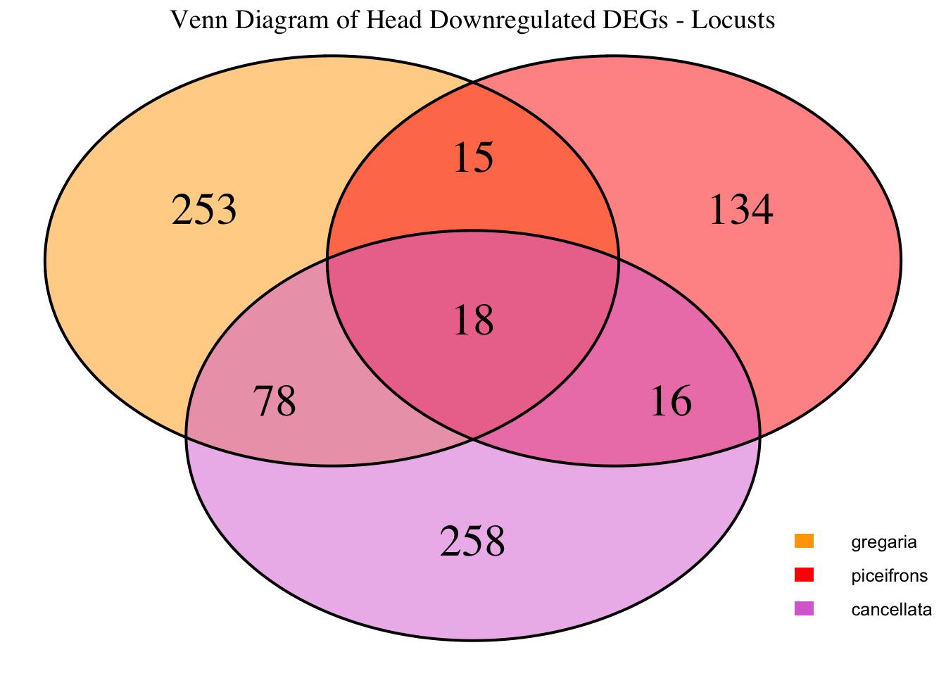
# Display the Venn diagram and datatable for all significant DEGs
display_venn_with_datatable(venn_data_all, "Venn Diagram of All Significant DEGs - Locusts", allspecies_df)
# Define the species for Group 1
locusts <- c("gregaria", "piceifrons", "cancellata")
# Initialize an empty list to store heatmap data for each species
heatmap_list <- list()
# Loop through each species to process their data
for (species in locusts) {
# Load DESeq2 results for head
head_file <- file.path(workDir, "DEG_results/Bulk_RNAseq/", paste0(species, "/Head/DESeq2_results_Head_", species,"_togregaria.csv"))
# Load the data using fread() for memory efficiency
head_data <- fread(head_file, data.table = FALSE)
# Check if data is empty and handle accordingly
if (nrow(head_data) == 0) {
message(paste("No data for species:", species))
next # Skip to the next species if there's no data
}
# Filter significant DEGs first (reduces memory use in sorting)
head_data_filtered <- head_data %>%
filter(padj < 0.05, abs(log2FoldChange) > 1) # Keep only strong up/downregulated DEGs
# Select top 500 upregulated and top 500 downregulated genes
head_up <- head_data_filtered %>%
filter(log2FoldChange > 1) %>%
arrange(desc(log2FoldChange)) %>%
slice_head(n = 500) # More memory-efficient than slice(1:500)
head_down <- head_data_filtered %>%
filter(log2FoldChange < -1) %>%
arrange(log2FoldChange) %>%
slice_head(n = 500) # More memory-efficient than slice(1:500)
# Combine data for heatmap, adding the species column
heatmap_data <- bind_rows(
head_up %>% mutate(Tissue = "Head", Regulation = "Upregulated", Species = species),
head_down %>% mutate(Tissue = "Head", Regulation = "Downregulated", Species = species)
) %>%
select(GeneID, log2FoldChange, Tissue, Regulation, Species)
# Append the heatmap data to the list
heatmap_list[[species]] <- heatmap_data
}
# Combine all species data into a single dataframe for heatmap matrix preparation
final_heatmap_data <- bind_rows(heatmap_list)
# Check if final_heatmap_data is empty before proceeding
if (nrow(final_heatmap_data) == 0) {
stop("No valid data available for heatmap generation.")
}
# **Fix duplicate GeneIDs: Aggregate log2FoldChange by taking the mean**
final_heatmap_data <- final_heatmap_data %>%
group_by(GeneID, Species) %>%
summarise(log2FoldChange = mean(log2FoldChange, na.rm = TRUE), .groups = "drop")
# **Create heatmap matrix without duplicates**
heatmap_matrix <- final_heatmap_data %>%
pivot_wider(names_from = Species, values_from = log2FoldChange, values_fill = 0) %>%
column_to_rownames("GeneID") %>%
as.matrix()
# Define color palettes
# Define a custom color gradient where 0 is black
custom_color_palette1 <- colorRampPalette(c("cyan", "cyan3", "black", "orange3", "orange"))(100)
# Define a custom color gradient where 0 is white
custom_color_palette2 <- colorRampPalette(c("blue3", "blue", "white", "red", "red3"))(100)
# Define color breaks so that black is exactly at 0
max_abs_lfc <- max(abs(heatmap_matrix), na.rm = TRUE) # Get max absolute log2FoldChange
color_breaks <- seq(-max_abs_lfc, max_abs_lfc, length.out = 100) # Symmetric scale
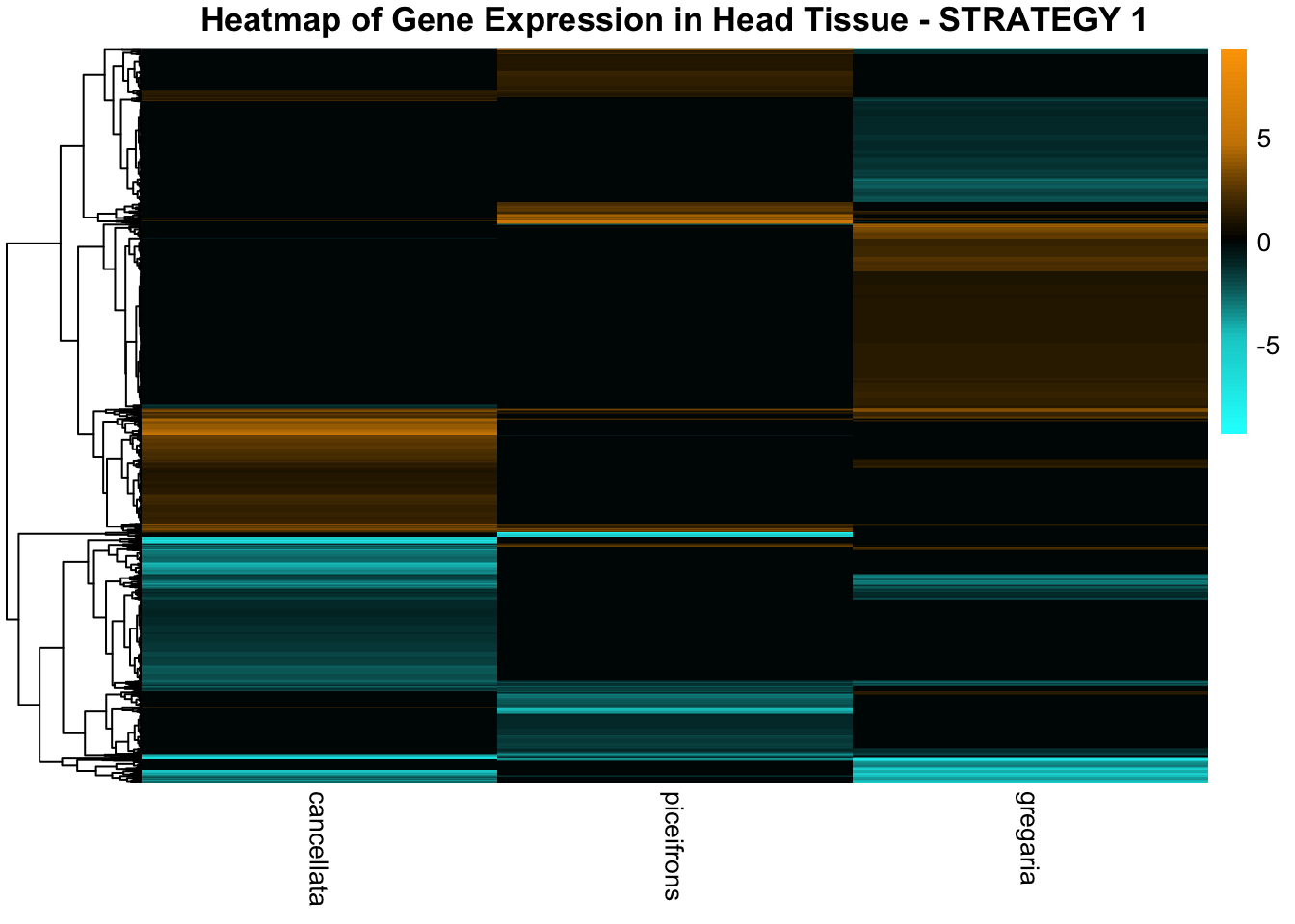
# Create heatmap with clustering
pheatmap(
heatmap_matrix,
color = custom_color_palette2,
breaks = color_breaks,
cluster_rows = TRUE, # Cluster genes
cluster_cols = FALSE, # Do not cluster species
show_rownames = FALSE,
show_colnames = TRUE,
fontsize_row = 6,
fontsize_col = 10,
main = "Heatmap of Gene Expression in Head Tissue - STRATEGY 1"
)
# Create heatmap without clustering columns
pheatmap(
  heatmap_matrix,
  color = custom_color_palette1,
  breaks = color_breaks,
  cluster_rows = TRUE,
  cluster_cols = FALSE,
  show_rownames = FALSE,
  show_colnames = TRUE,
  fontsize_row = 6,
  fontsize_col = 10,
  main = "Heatmap of Gene Expression in Head Tissue - STRATEGY 1"
)
Thorax tissues
# Define the species for Group 1
locusts <- c("gregaria", "piceifrons", "cancellata")

# Initialize an empty list to store DEG data
venn_data_locusts_up <- list()
venn_data_locusts_down <- list()
venn_data_locusts_all <- list()

# Function to load DEGs for a given group of species for thorax
load_deg_data <- function(species_list) {
  degs_up <- list()
  degs_down <- list()
  degs_all <- list()

  for (species in locusts) {
    thorax_file <- file.path(workDir, "DEG_results/Bulk_RNAseq/", paste0(species, "/Thorax/DESeq2_results_Thorax_", species,"_togregaria.csv"))

    thorax_data <- read.csv(thorax_file, stringsAsFactors = FALSE)

    # Check if data is empty and handle accordingly
    if (nrow(thorax_data) == 0) {
      message(paste("No data for species:", species))
      next  # Skip to the next species if there's no data
    }

    # Filter for significant DEGs (both upregulated and downregulated)
    thorax_up <- thorax_data %>%
      filter(padj < 0.05 & log2FoldChange >= 1) %>%
      select(GeneID = X)

    thorax_down <- thorax_data %>%
      filter(padj < 0.05 & log2FoldChange <= -1) %>%
      select(GeneID = X)

    all_deg <- thorax_data %>%
      filter(padj < 0.05 & abs(log2FoldChange) >= 1) %>%
      select(GeneID = X)

    # Store the DEGs in the list
    degs_up[[species]] <- thorax_up$GeneID
    degs_down[[species]] <- thorax_down$GeneID
    degs_all[[species]] <- all_deg$GeneID
  }

  return(list(up = degs_up, down = degs_down, all = degs_all))
}

# Load DEG data for Group 1 for thorax
venn_data_locusts <- load_deg_data(locusts)

# Prepare the data for the Venn diagrams
venn_data_up <- list(
  gregaria = venn_data_locusts$up[["gregaria"]],
  piceifrons = venn_data_locusts$up[["piceifrons"]],
  cancellata = venn_data_locusts$up[["cancellata"]]
)

venn_data_down <- list(
  gregaria = venn_data_locusts$down[["gregaria"]],
  piceifrons = venn_data_locusts$down[["piceifrons"]],
  cancellata = venn_data_locusts$down[["cancellata"]]
)

venn_data_all <- list(
  gregaria = venn_data_locusts$all[["gregaria"]],
  piceifrons = venn_data_locusts$all[["piceifrons"]],
  cancellata = venn_data_locusts$all[["cancellata"]]
)

# Function to display Venn diagram and corresponding datatable
display_venn_with_datatable <- function(venn_data, title, allspecies_df) {
  # Calculate the overlapping genes
  overlap_genes <- Reduce(intersect, venn_data)

  # Create a data frame for the overlapping genes
  overlap_df <- data.frame(GeneID = overlap_genes)

  # Merge to get species information
  meta_brock_df <- merge(overlap_df, allspecies_df, by = "GeneID", all.x = TRUE)

  # Generate the Venn diagram
  venn_plot <- venn.diagram(
    x = venn_data,
    category.names = c("gregaria", "piceifrons", "cancellata"),
    filename = NULL,
    output = TRUE,
    fill = c("orange", "red", "orchid"),  # Set colors for the groups
    alpha = 0.5,
    cex = 2,
    cat.cex = 0,
    main = title,
    main.cex = 1.2
  )

  # Clear the current plotting area before drawing the Venn diagram
  grid.newpage()

  # Display the Venn diagram
  grid.draw(venn_plot)

    # Manually create a custom legend
    legend_labels <- c("gregaria", "piceifrons", "cancellata")
    legend_colors <- c("orange", "red", "orchid")

    # Positioning the legend lower on the right side of the plot
    legend_x <- unit(0.85, "npc")  # Adjust x position
    legend_y <- unit(0.2, "npc")    # Lower the legend vertically

    # Draw the legend
    for (i in 1:length(legend_labels)) {
        grid.rect(x = legend_x, y = legend_y - unit((i - 1) * 0.05, "npc"),
                  width = unit(0.02, "npc"), height = unit(0.02, "npc"),
                  gp = gpar(fill = legend_colors[i], col = NA))
        grid.text(label = legend_labels[i], x = legend_x + unit(0.05, "npc"),
                  y = legend_y - unit((i - 1) * 0.05, "npc"),
                  just = "left", gp = gpar(cex = 0.8))
    }
  # Display the merged overlapping genes table with datatable
  datatable(meta_brock_df, options = list(
      pageLength = 10,
      scrollX = TRUE,
      autoWidth = TRUE,
      searchHighlight = TRUE
  ),
  rownames = FALSE,
  escape = FALSE
  ) %>%
  formatStyle(
      'Species', target = 'cell',
      fontStyle = 'italic'
  ) %>%
  formatStyle(
      columns = names(meta_brock_df),
      target = 'row',
      color = styleEqual(c("red", "blue", "black"), c("red", "blue", "black")),
      fontWeight = styleEqual(c("bold", "normal"), c("bold", "normal")),
      backgroundColor = styleEqual(c("red", "blue", "black"), c("white", "white", "white"))
  )
}

# Display the Venn diagram and datatable for thorax upregulated DEGs
display_venn_with_datatable(venn_data_up, "Venn Diagram of Thorax Upregulated DEGs - Locusts", allspecies_df)
# Display the Venn diagram and datatable for head downregulated DEGs
display_venn_with_datatable(venn_data_down, "Venn Diagram of Thorax Downregulated DEGs - Locusts", allspecies_df)
# Display the Venn diagram and datatable for all significant DEGs
display_venn_with_datatable(venn_data_all, "Venn Diagram of All Significant DEGs - Locusts", allspecies_df)
# Initialize an empty list to store heatmap data for each species
heatmap_list <- list()
# Loop through each species to process their data
for (species in locusts) {
# Load DESeq2 results for thorax
thorax_file <- file.path(workDir, "DEG_results/Bulk_RNAseq/", paste0(species, "/Thorax/DESeq2_results_Thorax_", species,"_togregaria.csv"))
# Load the data using fread() for memory efficiency
thorax_data <- fread(thorax_file, data.table = FALSE)
# Check if data is empty and handle accordingly
if (nrow(thorax_data) == 0) {
message(paste("No data for species:", species))
next # Skip to the next species if there's no data
}
# Filter significant DEGs first (reduces memory use in sorting)
thorax_data_filtered <- thorax_data %>%
filter(padj < 0.05, abs(log2FoldChange) > 1) # Keep only strong up/downregulated DEGs
# Select top 500 upregulated and top 500 downregulated genes
thorax_up <- thorax_data_filtered %>%
filter(log2FoldChange > 1) %>%
arrange(desc(log2FoldChange)) %>%
slice_head(n = 500) # More memory-efficient than slice(1:500)
thorax_down <- thorax_data_filtered %>%
filter(log2FoldChange < -1) %>%
arrange(log2FoldChange) %>%
slice_head(n = 500) # More memory-efficient than slice(1:500)
# Combine data for heatmap, adding the species column
heatmap_data <- bind_rows(
thorax_up %>% mutate(Tissue = "Thorax", Regulation = "Upregulated", Species = species),
thorax_down %>% mutate(Tissue = "Thorax", Regulation = "Downregulated", Species = species)
) %>%
select(GeneID, log2FoldChange, Tissue, Regulation, Species)
# Append the heatmap data to the list
heatmap_list[[species]] <- heatmap_data
}
# Combine all species data into a single dataframe for heatmap matrix preparation
final_heatmap_data <- bind_rows(heatmap_list)
# Check if final_heatmap_data is empty before proceeding
if (nrow(final_heatmap_data) == 0) {
stop("No valid data available for heatmap generation.")
}
# **Fix duplicate GeneIDs: Aggregate log2FoldChange by taking the mean**
final_heatmap_data <- final_heatmap_data %>%
group_by(GeneID, Species) %>%
summarise(log2FoldChange = mean(log2FoldChange, na.rm = TRUE), .groups = "drop")
# **Create heatmap matrix without duplicates**
heatmap_matrix <- final_heatmap_data %>%
pivot_wider(names_from = Species, values_from = log2FoldChange, values_fill = 0) %>%
column_to_rownames("GeneID") %>%
as.matrix()
# Define color palettes
# Define a custom color gradient where 0 is black
custom_color_palette1 <- colorRampPalette(c("cyan", "cyan3", "black", "orange3", "orange"))(100)
# Define a custom color gradient where 0 is white
custom_color_palette2 <- colorRampPalette(c("blue3", "blue", "white", "red", "red3"))(100)
# Define color breaks so that black is exactly at 0
max_abs_lfc <- max(abs(heatmap_matrix), na.rm = TRUE) # Get max absolute log2FoldChange
color_breaks <- seq(-max_abs_lfc, max_abs_lfc, length.out = 100) # Symmetric scale
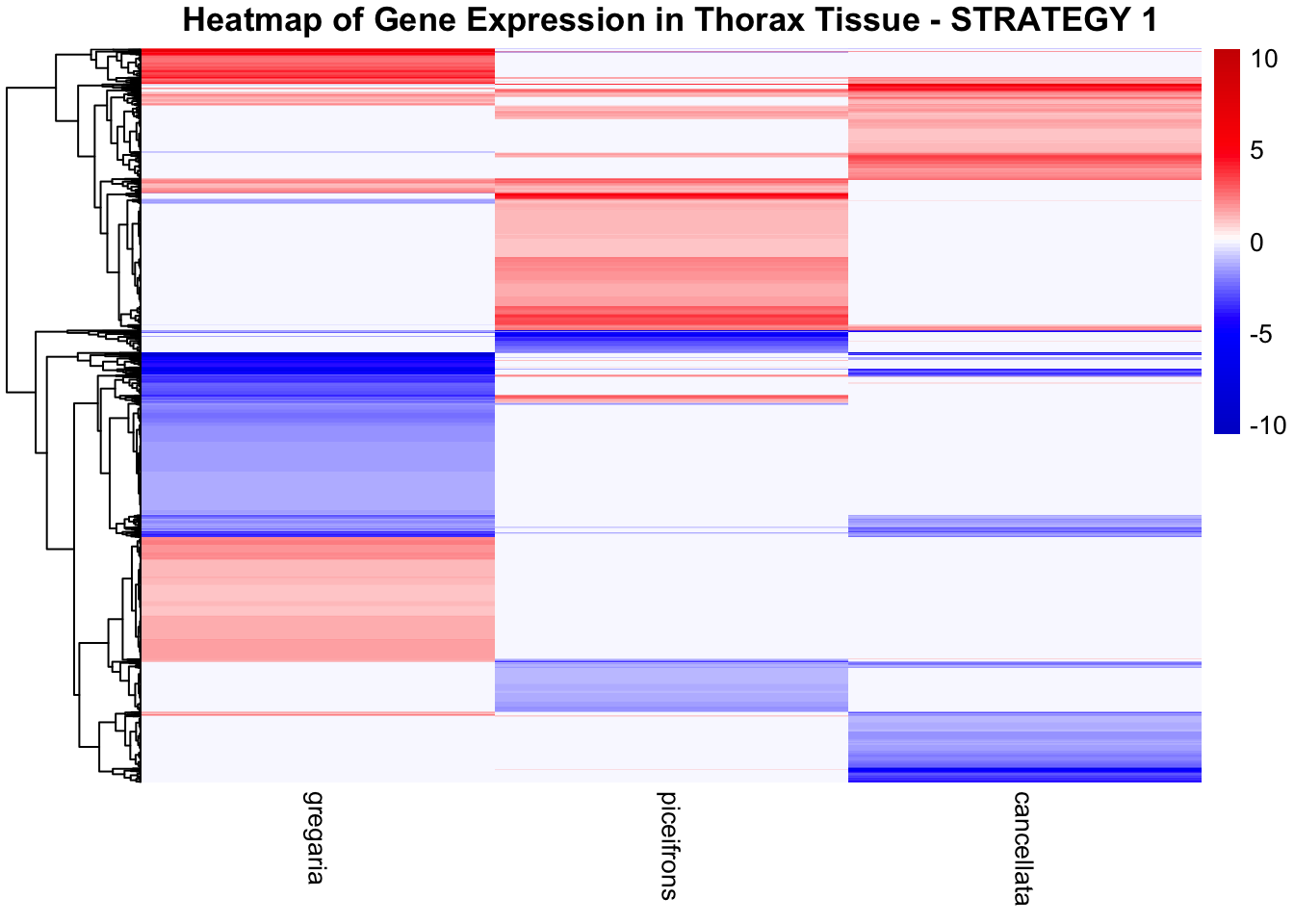
# Create heatmap with clustering
pheatmap(
heatmap_matrix,
color = custom_color_palette2,
breaks = color_breaks,
cluster_rows = TRUE, # Cluster genes
cluster_cols = FALSE, # Do not cluster species
show_rownames = FALSE,
show_colnames = TRUE,
fontsize_row = 6,
fontsize_col = 10,
main = "Heatmap of Gene Expression in Thorax Tissue - STRATEGY 1"
)
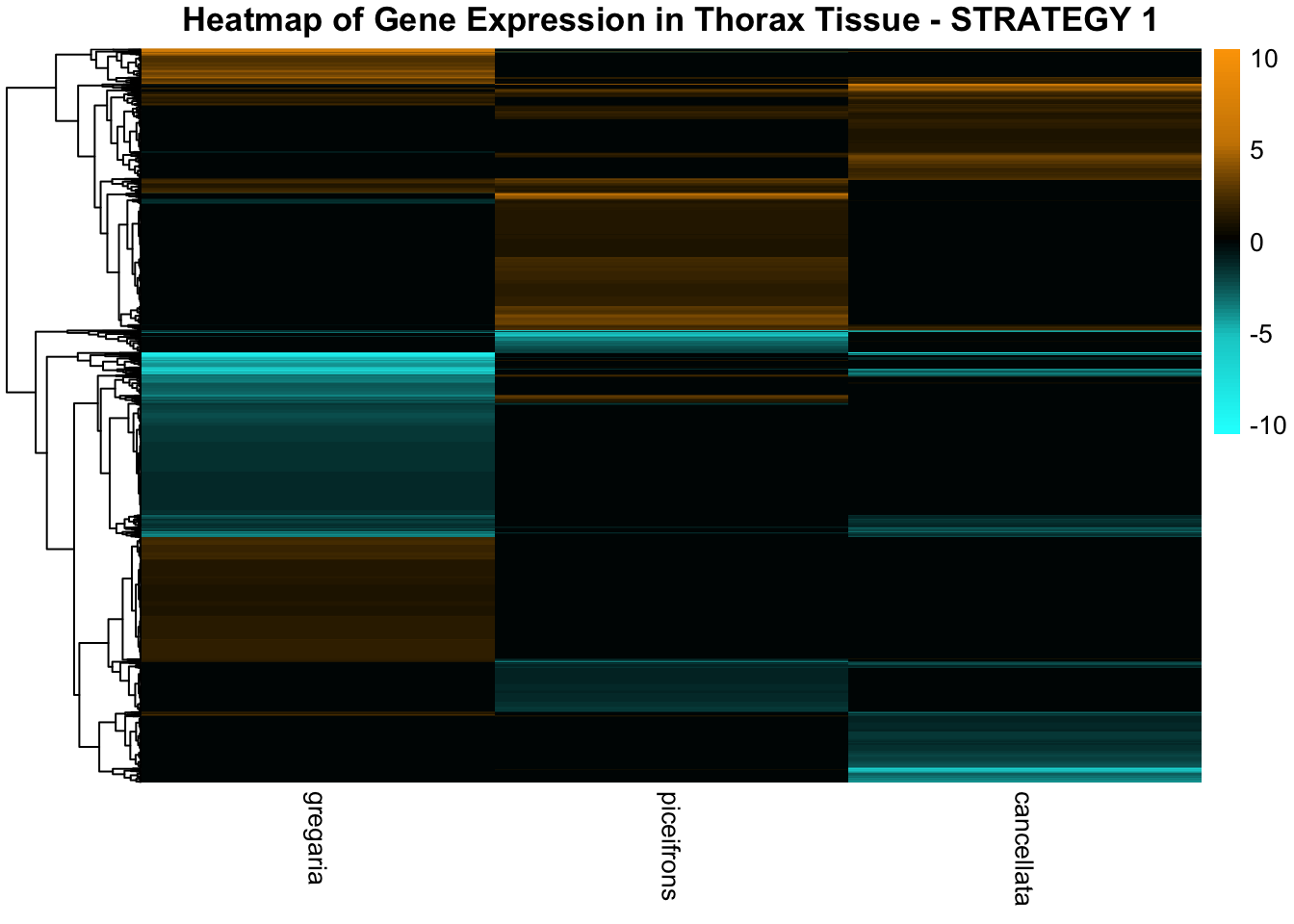
# Create heatmap without clustering columns
pheatmap(
  heatmap_matrix,
  color = custom_color_palette1,
  breaks = color_breaks,
  cluster_rows = TRUE,
  cluster_cols = FALSE,
  show_rownames = FALSE,
  show_colnames = TRUE,
  fontsize_row = 6,
  fontsize_col = 10,
  main = "Heatmap of Gene Expression in Thorax Tissue - STRATEGY 1"
)
piceifrons-americana-cubense
Head tissues
PACclade <- c("piceifrons", "americana", "cubense")

# Initialize an empty list to store DEG data
venn_data_PACclade_up <- list()
venn_data_PACclade_down <- list()
venn_data_PACclade_all <- list()

# Function to load DEGs for a given group of species for head
load_deg_data <- function(species_list) {
  degs_up <- list()
  degs_down <- list()
  degs_all <- list()

  for (species in PACclade) {
    head_file <- file.path(workDir, "DEG_results/Bulk_RNAseq/", paste0(species, "/Head/DESeq2_results_Head_", species,"_togregaria.csv"))

    head_data <- read.csv(head_file, stringsAsFactors = FALSE)

    # Check if data is empty and handle accordingly
    if (nrow(head_data) == 0) {
      message(paste("No data for species:", species))
      next  # Skip to the next species if there's no data
    }

    # Filter for significant DEGs (both upregulated and downregulated)
    head_up <- head_data %>%
      filter(padj < 0.05 & log2FoldChange >= 1) %>%
      select(GeneID = X)

    head_down <- head_data %>%
      filter(padj < 0.05 & log2FoldChange <= -1) %>%
      select(GeneID = X)

    all_deg <- head_data %>%
      filter(padj < 0.05 & abs(log2FoldChange) >= 1) %>%
      select(GeneID = X)

    # Store the DEGs in the list
    degs_up[[species]] <- head_up$GeneID
    degs_down[[species]] <- head_down$GeneID
    degs_all[[species]] <- all_deg$GeneID
  }

  return(list(up = degs_up, down = degs_down, all = degs_all))
}

# Load DEG data for Group 1 for head
venn_data_PACclade <- load_deg_data(PACclade)

# Prepare the data for the Venn diagrams
venn_data_up <- list(
  piceifrons = venn_data_PACclade$up[["piceifrons"]],
  americana = venn_data_PACclade$up[["americana"]],
  cubense = venn_data_PACclade$up[["cubense"]]
)

venn_data_down <- list(
  piceifrons = venn_data_PACclade$down[["piceifrons"]],
  americana = venn_data_PACclade$down[["americana"]],
  cubense = venn_data_PACclade$down[["cubense"]]
)

venn_data_all <- list(
  piceifrons = venn_data_PACclade$all[["piceifrons"]],
  americana = venn_data_PACclade$all[["americana"]],
  cubense = venn_data_PACclade$all[["cubense"]]
)

# Function to display Venn diagram and corresponding datatable
display_venn_with_datatable <- function(venn_data, title, allspecies_df) {
  # Calculate the overlapping genes
  overlap_genes <- Reduce(intersect, venn_data)

  # Create a data frame for the overlapping genes
  overlap_df <- data.frame(GeneID = overlap_genes)

  # Merge to get species information
  meta_brock_df <- merge(overlap_df, allspecies_df, by = "GeneID", all.x = TRUE)

  # Generate the Venn diagram
  venn_plot <- venn.diagram(
    x = venn_data,
    category.names = c("piceifrons", "americana", "cubense"),
    filename = NULL,
    output = TRUE,
    fill = c("red", "green", "yellow"),  # Set colors for the groups
    alpha = 0.5,
    cex = 2,
    cat.cex = 0,
    main = title,
    main.cex = 1.2
  )

  # Clear the current plotting area before drawing the Venn diagram
  grid.newpage()

  # Display the Venn diagram
  grid.draw(venn_plot)

    # Manually create a custom legend
    legend_labels <- c("piceifrons", "americana", "cubense")
    legend_colors <- c("red", "green", "yellow")

    # Positioning the legend lower on the right side of the plot
    legend_x <- unit(0.85, "npc")  # Adjust x position
    legend_y <- unit(0.2, "npc")    # Lower the legend vertically

    # Draw the legend
    for (i in 1:length(legend_labels)) {
        grid.rect(x = legend_x, y = legend_y - unit((i - 1) * 0.05, "npc"),
                  width = unit(0.02, "npc"), height = unit(0.02, "npc"),
                  gp = gpar(fill = legend_colors[i], col = NA))
        grid.text(label = legend_labels[i], x = legend_x + unit(0.05, "npc"),
                  y = legend_y - unit((i - 1) * 0.05, "npc"),
                  just = "left", gp = gpar(cex = 0.8))
    }
  # Display the merged overlapping genes table with datatable
  datatable(meta_brock_df, options = list(
      pageLength = 10,
      scrollX = TRUE,
      autoWidth = TRUE,
      searchHighlight = TRUE
  ),
  rownames = FALSE,
  escape = FALSE
  ) %>%
  formatStyle(
      'Species', target = 'cell',
      fontStyle = 'italic'
  ) %>%
  formatStyle(
      columns = names(meta_brock_df),
      target = 'row',
      color = styleEqual(c("red", "blue", "black"), c("red", "blue", "black")),
      fontWeight = styleEqual(c("bold", "normal"), c("bold", "normal")),
      backgroundColor = styleEqual(c("red", "blue", "black"), c("white", "white", "white"))
  )
}

# Display the Venn diagram and datatable for head upregulated DEGs
display_venn_with_datatable(venn_data_up, "Venn Diagram of Head Upregulated DEGs - PACclade", allspecies_df)
# Display the Venn diagram and datatable for head downregulated DEGs
display_venn_with_datatable(venn_data_down, "Venn Diagram of Head Downregulated DEGs - PACclade", allspecies_df)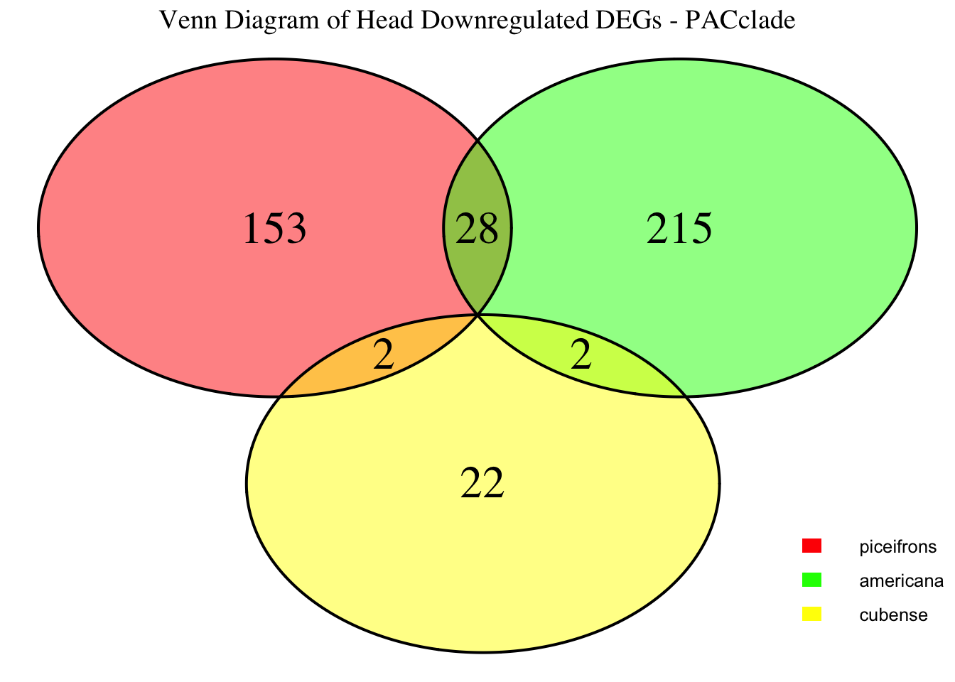
# Display the Venn diagram and datatable for all significant DEGs
display_venn_with_datatable(venn_data_all, "Venn Diagram of All Significant DEGs - PACclade", allspecies_df)
# Define the species for Group 1
PACclade <- c("piceifrons", "americana", "cubense")

# Initialize an empty list to store heatmap data for each species
heatmap_list <- list()

# Loop through each species to process their data
for (species in PACclade) {
  # Load DESeq2 results for head
  head_file <- file.path(workDir, "DEG_results/Bulk_RNAseq/", paste0(species, "/Head/DESeq2_results_Head_", species,"_togregaria.csv"))

  # Load the data using fread() for memory efficiency
  head_data <- fread(head_file, data.table = FALSE)

  # Check if data is empty and handle accordingly
  if (nrow(head_data) == 0) {
    message(paste("No data for species:", species))
    next  # Skip to the next species if there's no data
  }

  # Filter significant DEGs first (reduces memory use in sorting)
  head_data_filtered <- head_data %>%
    filter(padj < 0.05, abs(log2FoldChange) > 1)  # Keep only strong up/downregulated DEGs

  # Select top 500 upregulated and top 500 downregulated genes
  head_up <- head_data_filtered %>%
    filter(log2FoldChange > 1) %>%
    arrange(desc(log2FoldChange)) %>%
    slice_head(n = 500)   # More memory-efficient than slice(1:500)

  head_down <- head_data_filtered %>%
    filter(log2FoldChange < -1) %>%
    arrange(log2FoldChange) %>%
    slice_head(n = 500)   # More memory-efficient than slice(1:500)

  # Combine data for heatmap, adding the species column
  heatmap_data <- bind_rows(
    head_up %>% mutate(Tissue = "Head", Regulation = "Upregulated", Species = species),
    head_down %>% mutate(Tissue = "Head", Regulation = "Downregulated", Species = species)
  ) %>%
    select(GeneID, log2FoldChange, Tissue, Regulation, Species)

  # Append the heatmap data to the list
  heatmap_list[[species]] <- heatmap_data
}

# Combine all species data into a single dataframe for heatmap matrix preparation
final_heatmap_data <- bind_rows(heatmap_list)

# Check if final_heatmap_data is empty before proceeding
if (nrow(final_heatmap_data) == 0) {
  stop("No valid data available for heatmap generation.")
}

# Fix duplicate GeneIDs: Aggregate log2FoldChange by taking the mean**
final_heatmap_data <- final_heatmap_data %>%
  group_by(GeneID, Species) %>%
  summarise(log2FoldChange = mean(log2FoldChange, na.rm = TRUE), .groups = "drop")

# *Create heatmap matrix without duplicates**
heatmap_matrix <- final_heatmap_data %>%
  pivot_wider(names_from = Species, values_from = log2FoldChange, values_fill = 0) %>%
  column_to_rownames("GeneID") %>%
  as.matrix()

# Define color palettes
# Define a custom color gradient where 0 is black
custom_color_palette1 <- colorRampPalette(c("cyan", "cyan3", "black", "orange3", "orange"))(100)

# Define a custom color gradient where 0 is white
custom_color_palette2 <- colorRampPalette(c("blue3", "blue", "white", "red", "red3"))(100)

# Define color breaks so that black is exactly at 0
max_abs_lfc <- max(abs(heatmap_matrix), na.rm = TRUE)  # Get max absolute log2FoldChange
color_breaks <- seq(-max_abs_lfc, max_abs_lfc, length.out = 100)  # Symmetric scale

# Create heatmap with clustering
pheatmap(
  heatmap_matrix,
  color = custom_color_palette2,
  breaks = color_breaks,
  cluster_rows = TRUE,  # Cluster genes
  cluster_cols = FALSE,  # Do not cluster species
  show_rownames = FALSE,
  show_colnames = TRUE,
  fontsize_row = 6,
  fontsize_col = 10,
  main = "Heatmap of Gene Expression in Head Tissue - STRATEGY 1"
)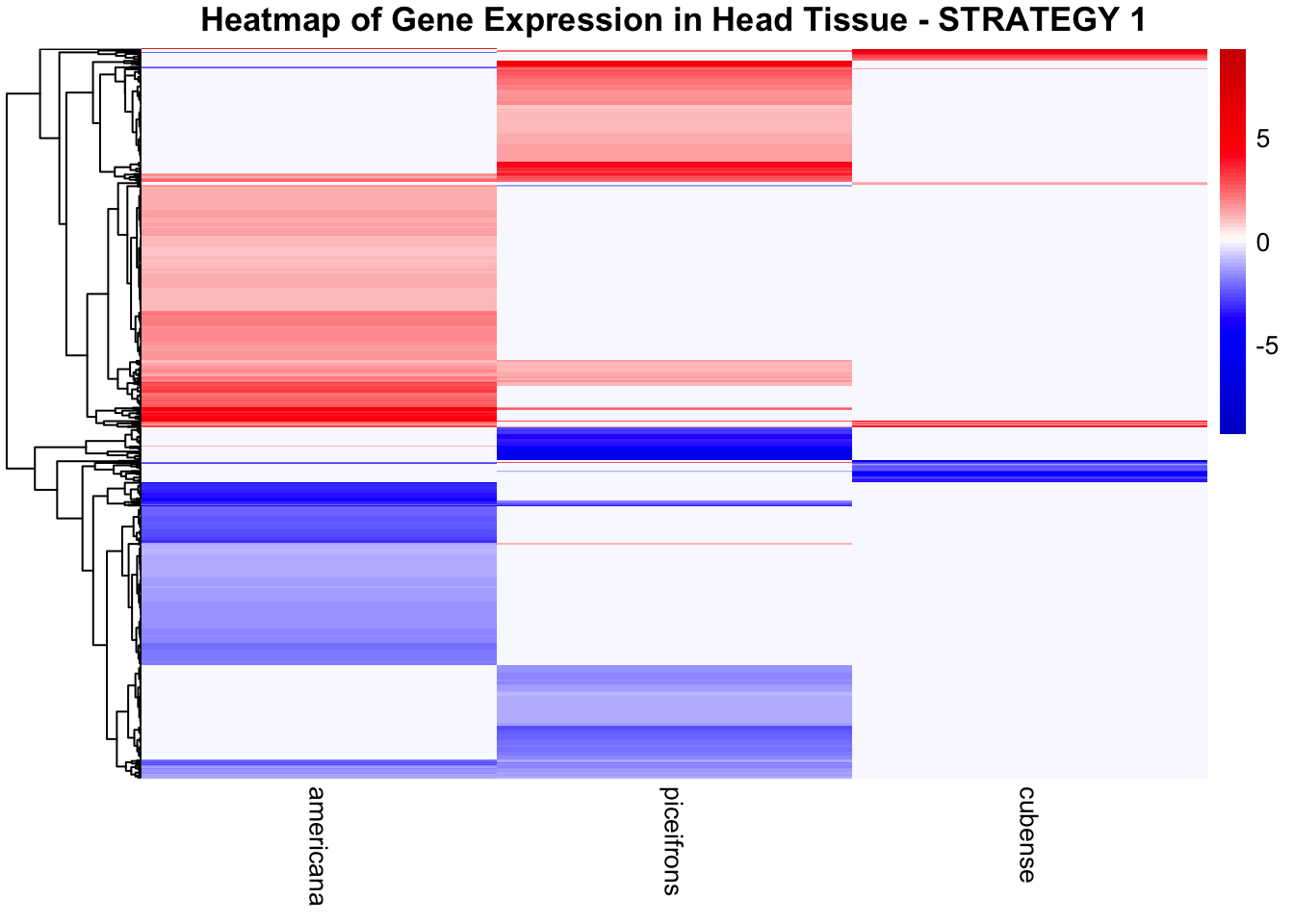
# Create heatmap without clustering columns
pheatmap(
  heatmap_matrix,
  color = custom_color_palette1,
  breaks = color_breaks,
  cluster_rows = TRUE,
  cluster_cols = FALSE,
  show_rownames = FALSE,
  show_colnames = TRUE,
  fontsize_row = 6,
  fontsize_col = 10,
  main = "Heatmap of Gene Expression in Head Tissue - STRATEGY 1"
)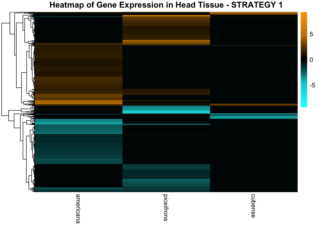
Thorax tissues
# Define the species for PACclade
PACclade <- c("piceifrons", "americana", "cubense")

# Initialize an empty list to store DEG data
venn_data_PACclade_up <- list()
venn_data_PACclade_down <- list()
venn_data_PACclade_all <- list()

# Function to load DEGs for a given group of species for thorax
load_deg_data <- function(species_list) {
  degs_up <- list()
  degs_down <- list()
  degs_all <- list()

  for (species in PACclade) {
    thorax_file <- file.path(workDir, "DEG_results/Bulk_RNAseq/", paste0(species, "/Thorax/DESeq2_results_Thorax_", species,"_togregaria.csv"))

    thorax_data <- read.csv(thorax_file, stringsAsFactors = FALSE)

    # Check if data is empty and handle accordingly
    if (nrow(thorax_data) == 0) {
      message(paste("No data for species:", species))
      next  # Skip to the next species if there's no data
    }

    # Filter for significant DEGs (both upregulated and downregulated)
    thorax_up <- thorax_data %>%
      filter(padj < 0.05 & log2FoldChange >= 1) %>%
      select(GeneID = X)

    thorax_down <- thorax_data %>%
      filter(padj < 0.05 & log2FoldChange <= -1) %>%
      select(GeneID = X)

    all_deg <- thorax_data %>%
      filter(padj < 0.05 & abs(log2FoldChange) >= 1) %>%
      select(GeneID = X)

    # Store the DEGs in the list
    degs_up[[species]] <- thorax_up$GeneID
    degs_down[[species]] <- thorax_down$GeneID
    degs_all[[species]] <- all_deg$GeneID
  }

  return(list(up = degs_up, down = degs_down, all = degs_all))
}

# Load DEG data for Group 1 for thorax
venn_data_PACclade <- load_deg_data(PACclade)

# Prepare the data for the Venn diagrams
venn_data_up <- list(
  piceifrons = venn_data_PACclade$up[["piceifrons"]],
  americana = venn_data_PACclade$up[["americana"]],
  cubense = venn_data_PACclade$up[["cubense"]]
)

venn_data_down <- list(
  piceifrons = venn_data_PACclade$down[["piceifrons"]],
  americana = venn_data_PACclade$down[["americana"]],
  cubense = venn_data_PACclade$down[["cubense"]]
)

venn_data_all <- list(
  piceifrons = venn_data_PACclade$all[["piceifrons"]],
  americana = venn_data_PACclade$all[["americana"]],
  cubense = venn_data_PACclade$all[["cubense"]]
)

# Function to display Venn diagram and corresponding datatable
display_venn_with_datatable <- function(venn_data, title, allspecies_df) {
  # Calculate the overlapping genes
  overlap_genes <- Reduce(intersect, venn_data)

  # Create a data frame for the overlapping genes
  overlap_df <- data.frame(GeneID = overlap_genes)

  # Merge to get species information
  meta_brock_df <- merge(overlap_df, allspecies_df, by = "GeneID", all.x = TRUE)

  # Generate the Venn diagram
  venn_plot <- venn.diagram(
    x = venn_data,
    category.names = c("piceifrons", "americana", "cubense"),
    filename = NULL,
    output = TRUE,
    fill = c("red", "green", "yellow"),   # Set colors for the groups
    alpha = 0.5,
    cex = 2,
    cat.cex = 0,
    main = title,
    main.cex = 1.2
  )

  # Clear the current plotting area before drawing the Venn diagram
  grid.newpage()

  # Display the Venn diagram
  grid.draw(venn_plot)

    # Manually create a custom legend
    legend_labels <- c("piceifrons", "americana", "cubense")
    legend_colors <- c("red", "green", "yellow")

    # Positioning the legend lower on the right side of the plot
    legend_x <- unit(0.85, "npc")  # Adjust x position
    legend_y <- unit(0.2, "npc")    # Lower the legend vertically

    # Draw the legend
    for (i in 1:length(legend_labels)) {
        grid.rect(x = legend_x, y = legend_y - unit((i - 1) * 0.05, "npc"),
                  width = unit(0.02, "npc"), height = unit(0.02, "npc"),
                  gp = gpar(fill = legend_colors[i], col = NA))
        grid.text(label = legend_labels[i], x = legend_x + unit(0.05, "npc"),
                  y = legend_y - unit((i - 1) * 0.05, "npc"),
                  just = "left", gp = gpar(cex = 0.8))
    }
  # Display the merged overlapping genes table with datatable
  datatable(meta_brock_df, options = list(
      pageLength = 10,
      scrollX = TRUE,
      autoWidth = TRUE,
      searchHighlight = TRUE
  ),
  rownames = FALSE,
  escape = FALSE
  ) %>%
  formatStyle(
      'Species', target = 'cell',
      fontStyle = 'italic'
  ) %>%
  formatStyle(
      columns = names(meta_brock_df),
      target = 'row',
      color = styleEqual(c("red", "blue", "black"), c("red", "blue", "black")),
      fontWeight = styleEqual(c("bold", "normal"), c("bold", "normal")),
      backgroundColor = styleEqual(c("red", "blue", "black"), c("white", "white", "white"))
  )
}

# Display the Venn diagram and datatable for thorax upregulated DEGs
display_venn_with_datatable(venn_data_up, "Venn Diagram of Thorax Upregulated DEGs - PACclade", allspecies_df)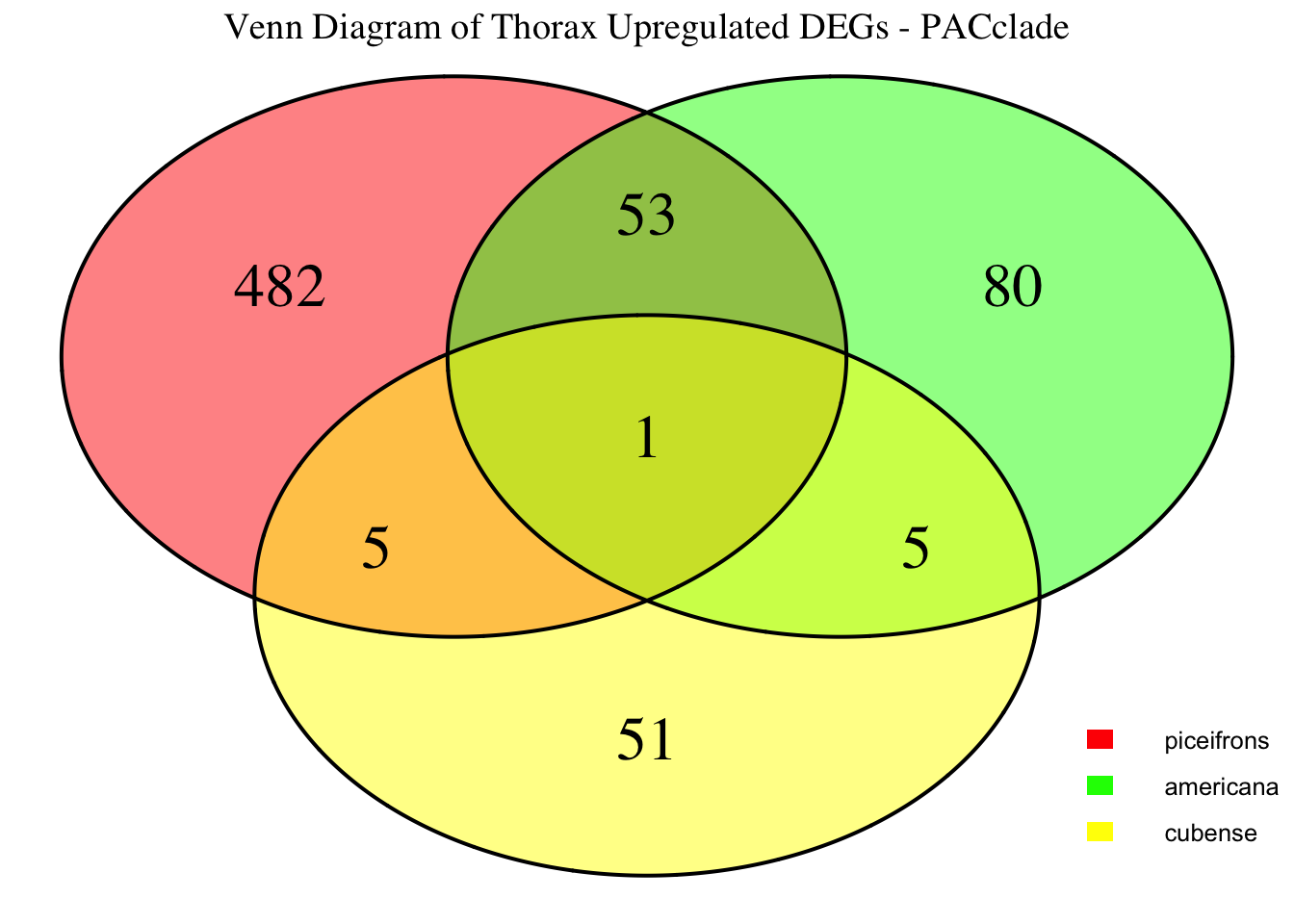
# Display the Venn diagram and datatable for head downregulated DEGs
display_venn_with_datatable(venn_data_down, "Venn Diagram of Thorax Downregulated DEGs - PACclade", allspecies_df)
# Display the Venn diagram and datatable for all significant DEGs
display_venn_with_datatable(venn_data_all, "Venn Diagram of All Significant DEGs - PACclade", allspecies_df)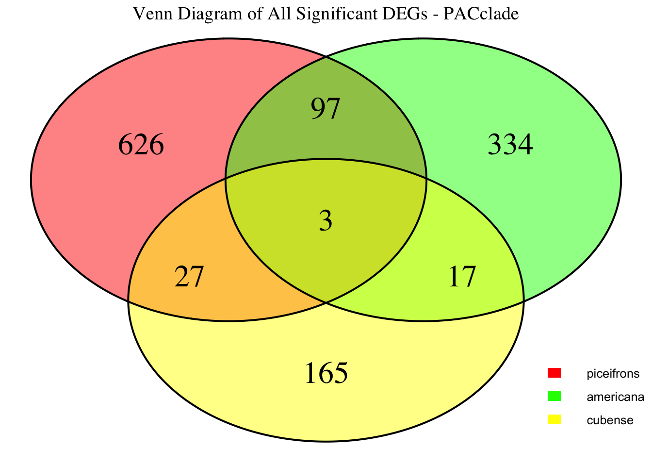
PACclade <- c("piceifrons", "americana", "cubense")

# Initialize an empty list to store heatmap data for each species
heatmap_list <- list()

# Loop through each species to process their data
for (species in PACclade) {
  # Load DESeq2 results for thorax
  thorax_file <- file.path(workDir, "DEG_results/Bulk_RNAseq/", paste0(species, "/Thorax/DESeq2_results_Thorax_", species,"_togregaria.csv"))

  # Load the data using fread() for memory efficiency
  thorax_data <- fread(thorax_file, data.table = FALSE)

  # Check if data is empty and handle accordingly
  if (nrow(thorax_data) == 0) {
    message(paste("No data for species:", species))
    next  # Skip to the next species if there's no data
  }

  # Filter significant DEGs first (reduces memory use in sorting)
  thorax_data_filtered <- thorax_data %>%
    filter(padj < 0.05, abs(log2FoldChange) > 1)  # Keep only strong up/downregulated DEGs

  # Select top 500 upregulated and top 500 downregulated genes
  thorax_up <- thorax_data_filtered %>%
    filter(log2FoldChange > 1) %>%
    arrange(desc(log2FoldChange)) %>%
    slice_head(n = 500)   # More memory-efficient than slice(1:500)

  thorax_down <- thorax_data_filtered %>%
    filter(log2FoldChange < -1) %>%
    arrange(log2FoldChange) %>%
    slice_head(n = 500)   # More memory-efficient than slice(1:500)

  # Combine data for heatmap, adding the species column
  heatmap_data <- bind_rows(
    thorax_up %>% mutate(Tissue = "Thorax", Regulation = "Upregulated", Species = species),
    thorax_down %>% mutate(Tissue = "Thorax", Regulation = "Downregulated", Species = species)
  ) %>%
    select(GeneID, log2FoldChange, Tissue, Regulation, Species)

  # Append the heatmap data to the list
  heatmap_list[[species]] <- heatmap_data
}

# Combine all species data into a single dataframe for heatmap matrix preparation
final_heatmap_data <- bind_rows(heatmap_list)

# Check if final_heatmap_data is empty before proceeding
if (nrow(final_heatmap_data) == 0) {
  stop("No valid data available for heatmap generation.")
}

# Fix duplicate GeneIDs: Aggregate log2FoldChange by taking the mean**
final_heatmap_data <- final_heatmap_data %>%
  group_by(GeneID, Species) %>%
  summarise(log2FoldChange = mean(log2FoldChange, na.rm = TRUE), .groups = "drop")

# *Create heatmap matrix without duplicates**
heatmap_matrix <- final_heatmap_data %>%
  pivot_wider(names_from = Species, values_from = log2FoldChange, values_fill = 0) %>%
  column_to_rownames("GeneID") %>%
  as.matrix()

# Define color palettes
# Define a custom color gradient where 0 is black
custom_color_palette1 <- colorRampPalette(c("cyan", "cyan3", "black", "orange3", "orange"))(100)

# Define a custom color gradient where 0 is white
custom_color_palette2 <- colorRampPalette(c("blue3", "blue", "white", "red", "red3"))(100)

# Define color breaks so that black is exactly at 0
max_abs_lfc <- max(abs(heatmap_matrix), na.rm = TRUE)  # Get max absolute log2FoldChange
color_breaks <- seq(-max_abs_lfc, max_abs_lfc, length.out = 100)  # Symmetric scale

# Create heatmap with clustering
pheatmap(
  heatmap_matrix,
  color = custom_color_palette2,
  breaks = color_breaks,
  cluster_rows = TRUE,  # Cluster genes
  cluster_cols = FALSE,  # Do not cluster species
  show_rownames = FALSE,
  show_colnames = TRUE,
  fontsize_row = 6,
  fontsize_col = 10,
  main = "Heatmap of Gene Expression in Thorax Tissue - STRATEGY 1"
)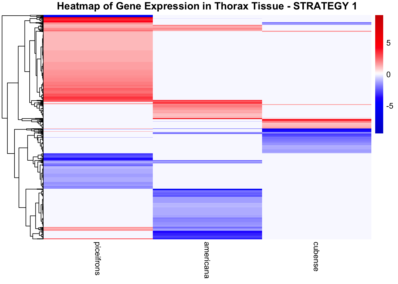
# Create heatmap without clustering columns
pheatmap(
  heatmap_matrix,
  color = custom_color_palette1,
  breaks = color_breaks,
  cluster_rows = TRUE,
  cluster_cols = FALSE,
  show_rownames = FALSE,
  show_colnames = TRUE,
  fontsize_row = 6,
  fontsize_col = 10,
  main = "Heatmap of Gene Expression in Thorax Tissue - STRATEGY 1"
)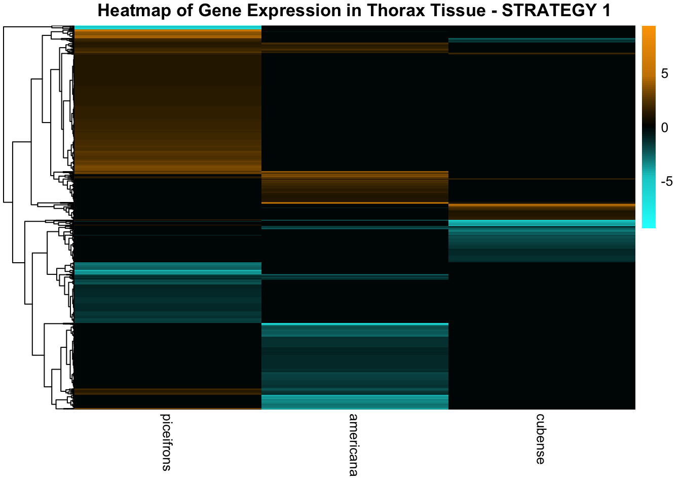
Plastic species
Head tissues
# Define the species for Group 1
plastic_species <- c("gregaria", "piceifrons", "cancellata","americana")

# Initialize an empty list to store DEG data
venn_data_plastic_species_up <- list()
venn_data_plastic_species_down <- list()
venn_data_plastic_species_all <- list()

# Function to load DEGs for a given group of species for head
load_deg_data <- function(species_list) {
  degs_up <- list()
  degs_down <- list()
  degs_all <- list()

  for (species in plastic_species) {
    head_file <- file.path(workDir, "DEG_results/Bulk_RNAseq/", paste0(species, "/Head/DESeq2_results_Head_", species,"_togregaria.csv"))

    head_data <- read.csv(head_file, stringsAsFactors = FALSE)

    # Check if data is empty and handle accordingly
    if (nrow(head_data) == 0) {
      message(paste("No data for species:", species))
      next  # Skip to the next species if there's no data
    }

    # Filter for significant DEGs (both upregulated and downregulated)
    head_up <- head_data %>%
      filter(padj < 0.05 & log2FoldChange >= 1) %>%
      select(GeneID = X)

    head_down <- head_data %>%
      filter(padj < 0.05 & log2FoldChange <= -1) %>%
      select(GeneID = X)

    all_deg <- head_data %>%
      filter(padj < 0.05 & abs(log2FoldChange) >= 1) %>%
      select(GeneID = X)

    # Store the DEGs in the list
    degs_up[[species]] <- head_up$GeneID
    degs_down[[species]] <- head_down$GeneID
    degs_all[[species]] <- all_deg$GeneID
  }

  return(list(up = degs_up, down = degs_down, all = degs_all))
}

# Load DEG data for Group 1 for head
venn_data_plastic_species <- load_deg_data(plastic_species)

# Prepare the data for the Venn diagrams
venn_data_up <- list(
  gregaria = venn_data_plastic_species$up[["gregaria"]],
  piceifrons = venn_data_plastic_species$up[["piceifrons"]],
  cancellata = venn_data_plastic_species$up[["cancellata"]],
  americana = venn_data_plastic_species$up[["americana"]]
)

venn_data_down <- list(
  gregaria = venn_data_plastic_species$down[["gregaria"]],
  piceifrons = venn_data_plastic_species$down[["piceifrons"]],
  cancellata = venn_data_plastic_species$down[["cancellata"]],
  americana = venn_data_plastic_species$down[["americana"]]
)

venn_data_all <- list(
  gregaria = venn_data_plastic_species$all[["gregaria"]],
  piceifrons = venn_data_plastic_species$all[["piceifrons"]],
  cancellata = venn_data_plastic_species$all[["cancellata"]],
  americana = venn_data_plastic_species$all[["americana"]]
)

# Function to display Venn diagram and corresponding datatable
display_venn_with_datatable <- function(venn_data, title, allspecies_df) {
  # Calculate the overlapping genes
  overlap_genes <- Reduce(intersect, venn_data)

  # Create a data frame for the overlapping genes
  overlap_df <- data.frame(GeneID = overlap_genes)

  # Merge to get species information
  meta_brock_df <- merge(overlap_df, allspecies_df, by = "GeneID", all.x = TRUE)

  # Generate the Venn diagram
  venn_plot <- venn.diagram(
    x = venn_data,
    category.names = c("gregaria", "piceifrons", "cancellata","americana"),
    filename = NULL,
    output = TRUE,
    fill = c("orange", "red", "orchid", "green"),  # Set colors for the groups
    alpha = 0.5,
    cex = 2,
    cat.cex = 0,
    main = title,
    main.cex = 1.2
  )

  # Clear the current plotting area before drawing the Venn diagram
  grid.newpage()

  # Display the Venn diagram
  grid.draw(venn_plot)

    # Manually create a custom legend
    legend_labels <- c("gregaria", "piceifrons", "cancellata","americana")
    legend_colors <- c("orange", "red", "orchid", "green")

    # Positioning the legend lower on the right side of the plot
    legend_x <- unit(0.85, "npc")  # Adjust x position
    legend_y <- unit(0.2, "npc")    # Lower the legend vertically

    # Draw the legend
    for (i in 1:length(legend_labels)) {
        grid.rect(x = legend_x, y = legend_y - unit((i - 1) * 0.05, "npc"),
                  width = unit(0.02, "npc"), height = unit(0.02, "npc"),
                  gp = gpar(fill = legend_colors[i], col = NA))
        grid.text(label = legend_labels[i], x = legend_x + unit(0.05, "npc"),
                  y = legend_y - unit((i - 1) * 0.05, "npc"),
                  just = "left", gp = gpar(cex = 0.8))
    }
  # Display the merged overlapping genes table with datatable
  datatable(meta_brock_df, options = list(
      pageLength = 10,
      scrollX = TRUE,
      autoWidth = TRUE,
      searchHighlight = TRUE
  ),
  rownames = FALSE,
  escape = FALSE
  ) %>%
  formatStyle(
      'Species', target = 'cell',
      fontStyle = 'italic'
  ) %>%
  formatStyle(
      columns = names(meta_brock_df),
      target = 'row',
      color = styleEqual(c("red", "blue", "black"), c("red", "blue", "black")),
      fontWeight = styleEqual(c("bold", "normal"), c("bold", "normal")),
      backgroundColor = styleEqual(c("red", "blue", "black"), c("white", "white", "white"))
  )
}

# Display the Venn diagram and datatable for head upregulated DEGs
display_venn_with_datatable(venn_data_up, "Venn Diagram of Head Upregulated DEGs - plastic_species", allspecies_df)
# Display the Venn diagram and datatable for head downregulated DEGs
display_venn_with_datatable(venn_data_down, "Venn Diagram of Head Downregulated DEGs - plastic_species", allspecies_df)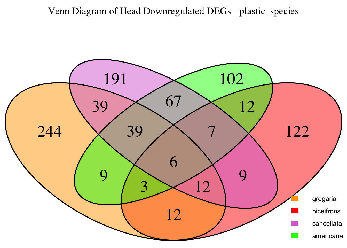
# Display the Venn diagram and datatable for all significant DEGs
display_venn_with_datatable(venn_data_all, "Venn Diagram of All Significant DEGs - plastic_species", allspecies_df)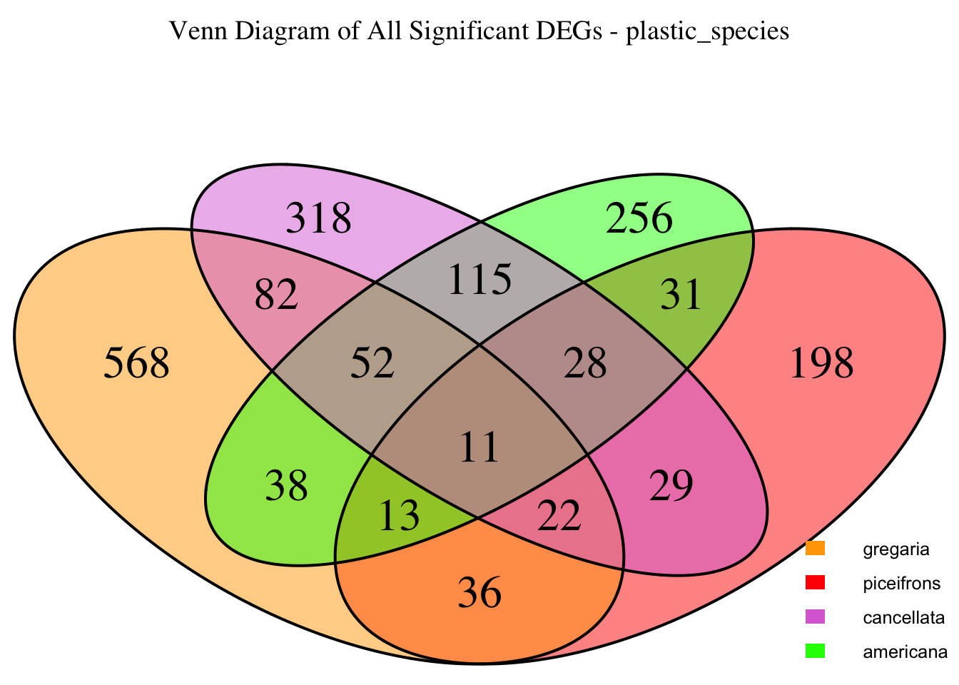
# Define the species for Group 1
plastic_species <- c("gregaria", "piceifrons", "cancellata","americana")

# Initialize an empty list to store heatmap data for each species
heatmap_list <- list()

# Loop through each species to process their data
for (species in locusts) {
  # Load DESeq2 results for head
  head_file <- file.path(workDir, "DEG_results/Bulk_RNAseq/", paste0(species, "/Head/DESeq2_results_Head_", species,"_togregaria.csv"))

  # Load the data using fread() for memory efficiency
  head_data <- fread(head_file, data.table = FALSE)

  # Check if data is empty and handle accordingly
  if (nrow(head_data) == 0) {
    message(paste("No data for species:", species))
    next  # Skip to the next species if there's no data
  }

  # Filter significant DEGs first (reduces memory use in sorting)
  head_data_filtered <- head_data %>%
    filter(padj < 0.05, abs(log2FoldChange) > 1)  # Keep only strong up/downregulated DEGs

  # Select top 500 upregulated and top 500 downregulated genes
  head_up <- head_data_filtered %>%
    filter(log2FoldChange > 1) %>%
    arrange(desc(log2FoldChange)) %>%
    slice_head(n = 500)   # More memory-efficient than slice(1:500)

  head_down <- head_data_filtered %>%
    filter(log2FoldChange < -1) %>%
    arrange(log2FoldChange) %>%
    slice_head(n = 500)   # More memory-efficient than slice(1:500)

  # Combine data for heatmap, adding the species column
  heatmap_data <- bind_rows(
    head_up %>% mutate(Tissue = "Head", Regulation = "Upregulated", Species = species),
    head_down %>% mutate(Tissue = "Head", Regulation = "Downregulated", Species = species)
  ) %>%
    select(GeneID, log2FoldChange, Tissue, Regulation, Species)

  # Append the heatmap data to the list
  heatmap_list[[species]] <- heatmap_data
}

# Combine all species data into a single dataframe for heatmap matrix preparation
final_heatmap_data <- bind_rows(heatmap_list)

# Check if final_heatmap_data is empty before proceeding
if (nrow(final_heatmap_data) == 0) {
  stop("No valid data available for heatmap generation.")
}

# **Fix duplicate GeneIDs: Aggregate log2FoldChange by taking the mean**
final_heatmap_data <- final_heatmap_data %>%
  group_by(GeneID, Species) %>%
  summarise(log2FoldChange = mean(log2FoldChange, na.rm = TRUE), .groups = "drop")

# **Create heatmap matrix without duplicates**
heatmap_matrix <- final_heatmap_data %>%
  pivot_wider(names_from = Species, values_from = log2FoldChange, values_fill = 0) %>%
  column_to_rownames("GeneID") %>%
  as.matrix()

# Define color palettes
# Define a custom color gradient where 0 is black
custom_color_palette1 <- colorRampPalette(c("cyan", "cyan3", "black", "orange3", "orange"))(100)

# Define a custom color gradient where 0 is white
custom_color_palette2 <- colorRampPalette(c("blue3", "blue", "white", "red", "red3"))(100)

# Define color breaks so that black is exactly at 0
max_abs_lfc <- max(abs(heatmap_matrix), na.rm = TRUE)  # Get max absolute log2FoldChange
color_breaks <- seq(-max_abs_lfc, max_abs_lfc, length.out = 100)  # Symmetric scale

# Create heatmap with clustering
pheatmap(
  heatmap_matrix,
  color = custom_color_palette2,
  breaks = color_breaks,
  cluster_rows = TRUE,  # Cluster genes
  cluster_cols = FALSE,  # Do not cluster species
  show_rownames = FALSE,
  show_colnames = TRUE,
  fontsize_row = 6,
  fontsize_col = 10,
  main = "Heatmap of Gene Expression in Head Tissue - STRATEGY 1"
)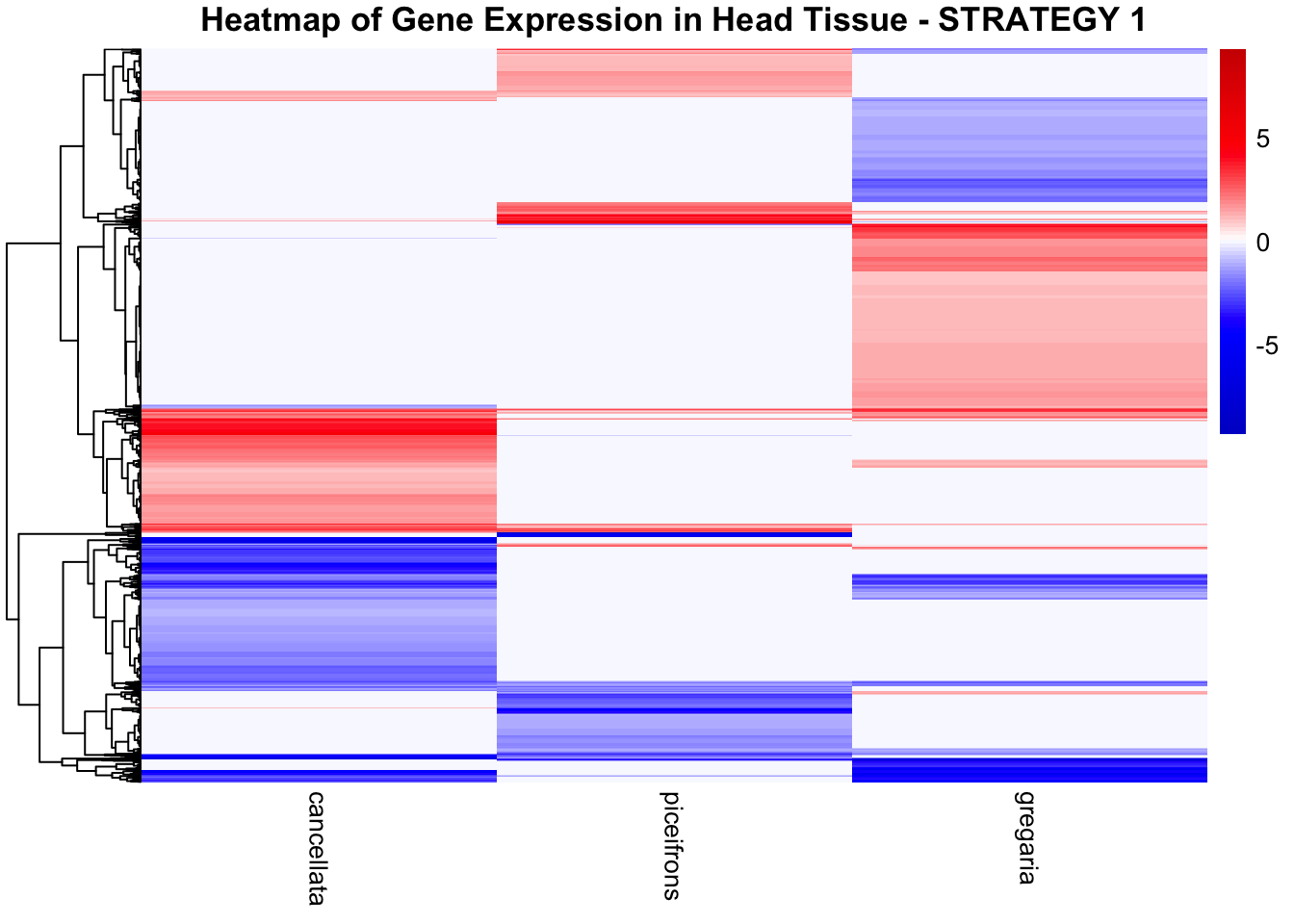
# Create heatmap without clustering columns
pheatmap(
  heatmap_matrix,
  color = custom_color_palette1,
  breaks = color_breaks,
  cluster_rows = TRUE,
  cluster_cols = FALSE,
  show_rownames = FALSE,
  show_colnames = TRUE,
  fontsize_row = 6,
  fontsize_col = 10,
  main = "Heatmap of Gene Expression in Head Tissue - STRATEGY 1"
)
Thorax tissues
plastic_species <- c("gregaria", "piceifrons", "cancellata","americana")

# Initialize an empty list to store DEG data
venn_data_plastic_species_up <- list()
venn_data_plastic_species_down <- list()
venn_data_plastic_species_all <- list()

# Function to load DEGs for a given group of species for thorax
load_deg_data <- function(species_list) {
  degs_up <- list()
  degs_down <- list()
  degs_all <- list()

  for (species in plastic_species) {
    thorax_file <- file.path(workDir, "DEG_results/Bulk_RNAseq/", paste0(species, "/Thorax/DESeq2_results_Thorax_", species,"_togregaria.csv"))

    thorax_data <- read.csv(thorax_file, stringsAsFactors = FALSE)

    # Check if data is empty and handle accordingly
    if (nrow(thorax_data) == 0) {
      message(paste("No data for species:", species))
      next  # Skip to the next species if there's no data
    }

    # Filter for significant DEGs (both upregulated and downregulated)
    thorax_up <- thorax_data %>%
      filter(padj < 0.05 & log2FoldChange >= 1) %>%
      select(GeneID = X)

    thorax_down <- thorax_data %>%
      filter(padj < 0.05 & log2FoldChange <= -1) %>%
      select(GeneID = X)

    all_deg <- thorax_data %>%
      filter(padj < 0.05 & abs(log2FoldChange) >= 1) %>%
      select(GeneID = X)

    # Store the DEGs in the list
    degs_up[[species]] <- thorax_up$GeneID
    degs_down[[species]] <- thorax_down$GeneID
    degs_all[[species]] <- all_deg$GeneID
  }

  return(list(up = degs_up, down = degs_down, all = degs_all))
}

# Load DEG data for Group 1 for thorax
venn_data_plastic_species <- load_deg_data(plastic_species)

# Prepare the data for the Venn diagrams
venn_data_up <- list(
  gregaria = venn_data_plastic_species$up[["gregaria"]],
  piceifrons = venn_data_plastic_species$up[["piceifrons"]],
  cancellata = venn_data_plastic_species$up[["cancellata"]],
  americana = venn_data_plastic_species$up[["americana"]]
)

venn_data_down <- list(
  gregaria = venn_data_plastic_species$down[["gregaria"]],
  piceifrons = venn_data_plastic_species$down[["piceifrons"]],
  cancellata = venn_data_plastic_species$down[["cancellata"]],
  americana = venn_data_plastic_species$down[["americana"]]
)

venn_data_all <- list(
  gregaria = venn_data_plastic_species$all[["gregaria"]],
  piceifrons = venn_data_plastic_species$all[["piceifrons"]],
  cancellata = venn_data_plastic_species$all[["cancellata"]],
  americana = venn_data_plastic_species$all[["americana"]]
)

# Function to display Venn diagram and corresponding datatable
display_venn_with_datatable <- function(venn_data, title, allspecies_df) {
  # Calculate the overlapping genes
  overlap_genes <- Reduce(intersect, venn_data)

  # Create a data frame for the overlapping genes
  overlap_df <- data.frame(GeneID = overlap_genes)

  # Merge to get species information
  meta_brock_df <- merge(overlap_df, allspecies_df, by = "GeneID", all.x = TRUE)

  # Generate the Venn diagram
  venn_plot <- venn.diagram(
    x = venn_data,
    category.names = c("gregaria", "piceifrons", "cancellata","americana"),
    filename = NULL,
    output = TRUE,
    fill = c("orange", "red", "orchid", "green"),  # Set colors for the groups
    alpha = 0.5,
    cex = 2,
    cat.cex = 0,
    main = title,
    main.cex = 1.2
  )

  # Clear the current plotting area before drawing the Venn diagram
  grid.newpage()

  # Display the Venn diagram
  grid.draw(venn_plot)

    # Manually create a custom legend
    legend_labels <- c("gregaria", "piceifrons", "cancellata","americana")
    legend_colors <- c("orange", "red", "orchid", "green")

    # Positioning the legend lower on the right side of the plot
    legend_x <- unit(0.85, "npc")  # Adjust x position
    legend_y <- unit(0.2, "npc")    # Lower the legend vertically

    # Draw the legend
    for (i in 1:length(legend_labels)) {
        grid.rect(x = legend_x, y = legend_y - unit((i - 1) * 0.05, "npc"),
                  width = unit(0.02, "npc"), height = unit(0.02, "npc"),
                  gp = gpar(fill = legend_colors[i], col = NA))
        grid.text(label = legend_labels[i], x = legend_x + unit(0.05, "npc"),
                  y = legend_y - unit((i - 1) * 0.05, "npc"),
                  just = "left", gp = gpar(cex = 0.8))
    }
  # Display the merged overlapping genes table with datatable
  datatable(meta_brock_df, options = list(
      pageLength = 10,
      scrollX = TRUE,
      autoWidth = TRUE,
      searchHighlight = TRUE
  ),
  rownames = FALSE,
  escape = FALSE
  ) %>%
  formatStyle(
      'Species', target = 'cell',
      fontStyle = 'italic'
  ) %>%
  formatStyle(
      columns = names(meta_brock_df),
      target = 'row',
      color = styleEqual(c("red", "blue", "black"), c("red", "blue", "black")),
      fontWeight = styleEqual(c("bold", "normal"), c("bold", "normal")),
      backgroundColor = styleEqual(c("red", "blue", "black"), c("white", "white", "white"))
  )
}

# Display the Venn diagram and datatable for thorax upregulated DEGs
display_venn_with_datatable(venn_data_up, "Venn Diagram of Thorax Upregulated DEGs - plastic_species", allspecies_df)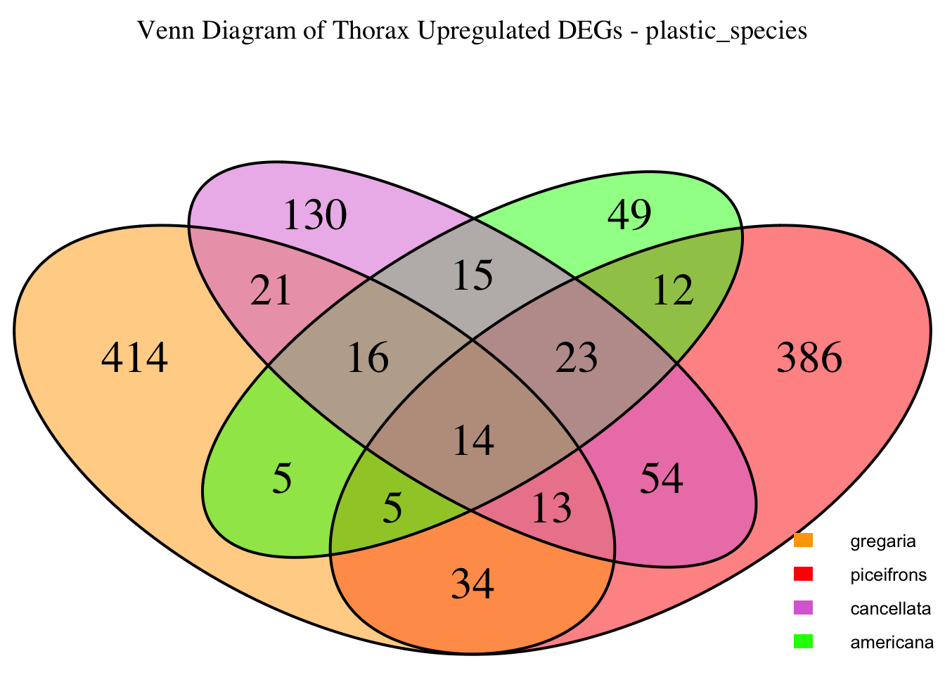
# Display the Venn diagram and datatable for thorax downregulated DEGs
display_venn_with_datatable(venn_data_down, "Venn Diagram of Thorax Downregulated DEGs - plastic_species", allspecies_df)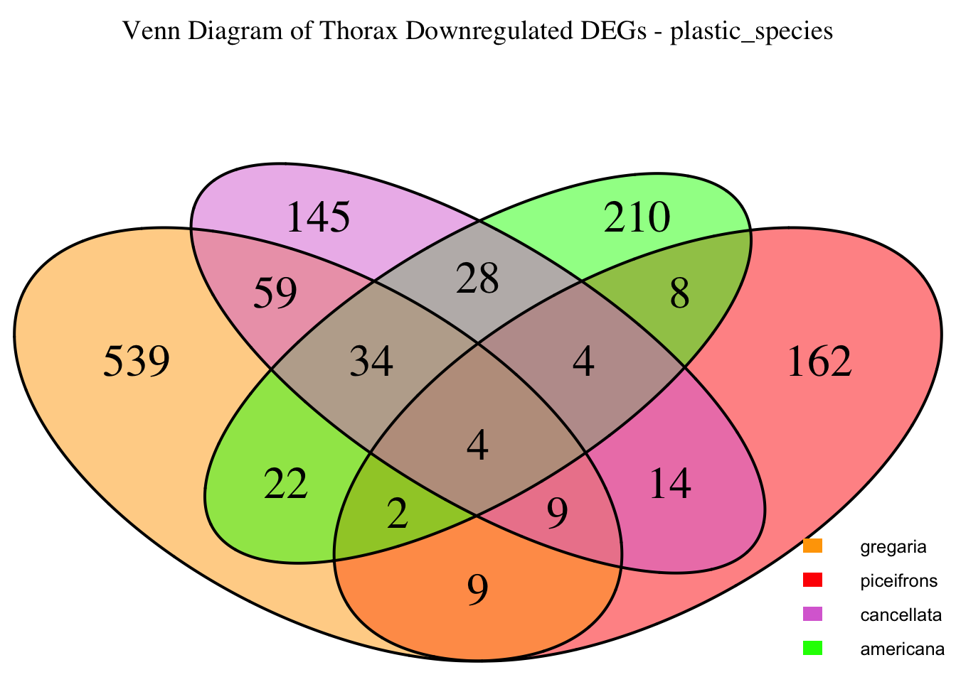
# Display the Venn diagram and datatable for all significant DEGs
display_venn_with_datatable(venn_data_all, "Venn Diagram of All Significant DEGs - plastic_species", allspecies_df)
plastic_species <- c("gregaria", "piceifrons", "cancellata","americana")

# Initialize an empty list to store heatmap data for each species
heatmap_list <- list()

# Loop through each species to process their data
for (species in plastic_species) {
  # Load DESeq2 results for thorax
  thorax_file <- file.path(workDir, "DEG_results/Bulk_RNAseq/", paste0(species, "/Thorax/DESeq2_results_Thorax_", species,"_togregaria.csv"))

  # Load the data using fread() for memory efficiency
  thorax_data <- fread(thorax_file, data.table = FALSE)

  # Check if data is empty and handle accordingly
  if (nrow(thorax_data) == 0) {
    message(paste("No data for species:", species))
    next  # Skip to the next species if there's no data
  }

  # Filter significant DEGs first (reduces memory use in sorting)
  thorax_data_filtered <- thorax_data %>%
    filter(padj < 0.05, abs(log2FoldChange) > 1)  # Keep only strong up/downregulated DEGs

  # Select top 500 upregulated and top 500 downregulated genes
  thorax_up <- thorax_data_filtered %>%
    filter(log2FoldChange > 1) %>%
    arrange(desc(log2FoldChange)) %>%
    slice_head(n = 500)   # More memory-efficient than slice(1:500)

  thorax_down <- thorax_data_filtered %>%
    filter(log2FoldChange < -1) %>%
    arrange(log2FoldChange) %>%
    slice_head(n = 500)   # More memory-efficient than slice(1:500)

  # Combine data for heatmap, adding the species column
  heatmap_data <- bind_rows(
    thorax_up %>% mutate(Tissue = "Thorax", Regulation = "Upregulated", Species = species),
    thorax_down %>% mutate(Tissue = "Thorax", Regulation = "Downregulated", Species = species)
  ) %>%
    select(GeneID, log2FoldChange, Tissue, Regulation, Species)

  # Append the heatmap data to the list
  heatmap_list[[species]] <- heatmap_data
}

# Combine all species data into a single dataframe for heatmap matrix preparation
final_heatmap_data <- bind_rows(heatmap_list)

# Check if final_heatmap_data is empty before proceeding
if (nrow(final_heatmap_data) == 0) {
  stop("No valid data available for heatmap generation.")
}

# Fix duplicate GeneIDs: Aggregate log2FoldChange by taking the mean**
final_heatmap_data <- final_heatmap_data %>%
  group_by(GeneID, Species) %>%
  summarise(log2FoldChange = mean(log2FoldChange, na.rm = TRUE), .groups = "drop")

# *Create heatmap matrix without duplicates**
heatmap_matrix <- final_heatmap_data %>%
  pivot_wider(names_from = Species, values_from = log2FoldChange, values_fill = 0) %>%
  column_to_rownames("GeneID") %>%
  as.matrix()

# Define color palettes
# Define a custom color gradient where 0 is black
custom_color_palette1 <- colorRampPalette(c("cyan", "cyan3", "black", "orange3", "orange"))(100)

# Define a custom color gradient where 0 is white
custom_color_palette2 <- colorRampPalette(c("blue3", "blue", "white", "red", "red3"))(100)

# Define color breaks so that black is exactly at 0
max_abs_lfc <- max(abs(heatmap_matrix), na.rm = TRUE)  # Get max absolute log2FoldChange
color_breaks <- seq(-max_abs_lfc, max_abs_lfc, length.out = 100)  # Symmetric scale

# Create heatmap with clustering
pheatmap(
  heatmap_matrix,
  color = custom_color_palette2,
  breaks = color_breaks,
  cluster_rows = TRUE,  # Cluster genes
  cluster_cols = FALSE,  # Do not cluster species
  show_rownames = FALSE,
  show_colnames = TRUE,
  fontsize_row = 6,
  fontsize_col = 10,
  main = "Heatmap of Gene Expression in Thorax Tissue - STRATEGY 1"
)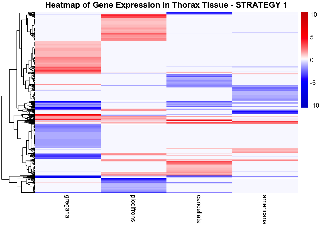
# Create heatmap without clustering columns
pheatmap(
  heatmap_matrix,
  color = custom_color_palette1,
  breaks = color_breaks,
  cluster_rows = TRUE,
  cluster_cols = FALSE,
  show_rownames = FALSE,
  show_colnames = TRUE,
  fontsize_row = 6,
  fontsize_col = 10,
  main = "Heatmap of Gene Expression in Thorax Tissue - STRATEGY 1"
)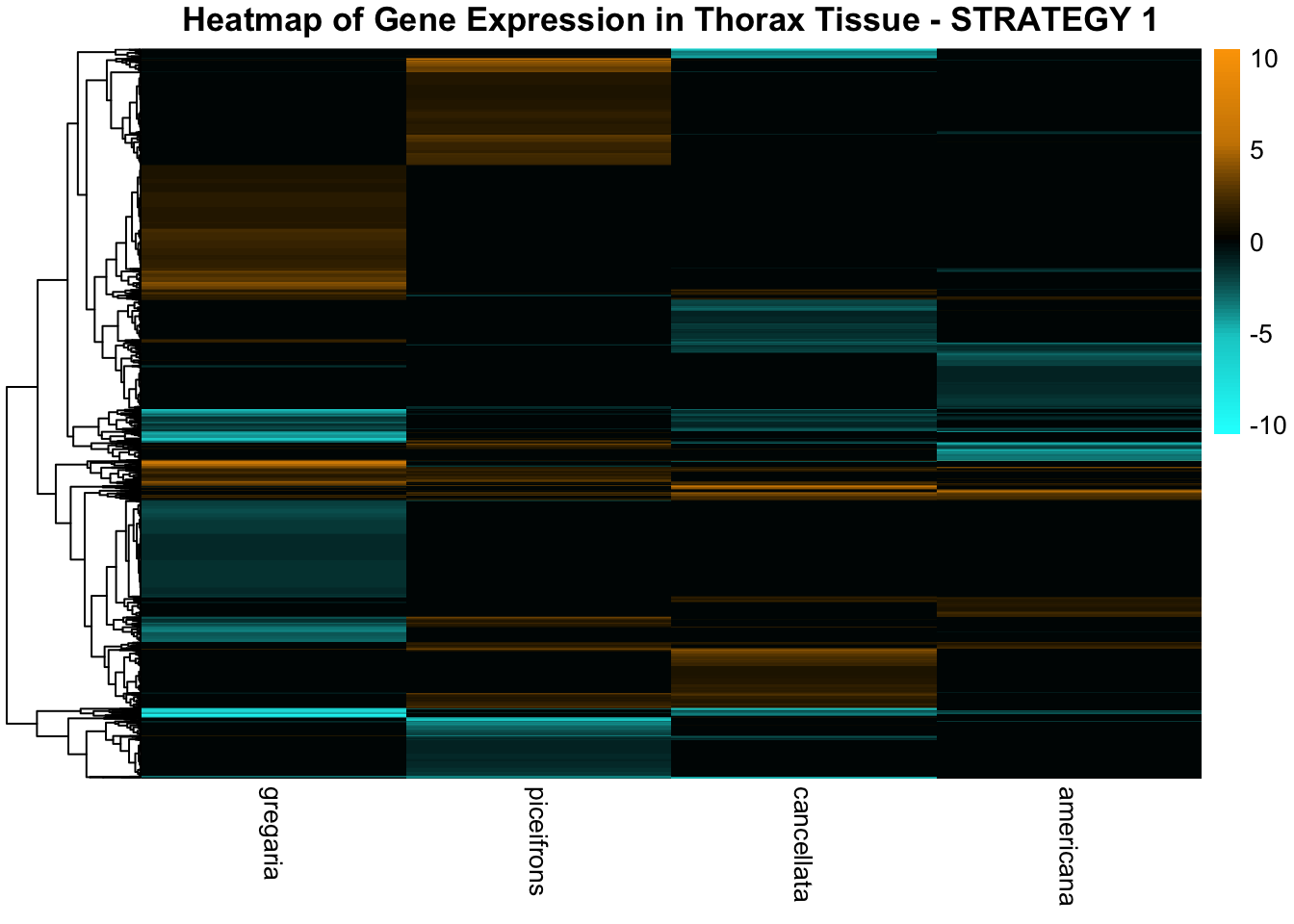
Five species
Combined tissues
# Define the species for Group 1
allspecies <- c("gregaria", "piceifrons", "cancellata","americana", "cubense")

# Initialize an empty list to store DEG data
venn_data_allspecies_up <- list()
venn_data_allspecies_down <- list()
venn_data_allspecies_all <- list()

# Function to load DEGs for a given group of species for head
load_deg_data <- function(species_list) {
  degs_up <- list()
  degs_down <- list()
  degs_all <- list()

  for (species in allspecies) {
    head_file <- file.path(workDir, "DEG_results/Bulk_RNAseq/", paste0(species, "/Head/DESeq2_results_Head_", species,"_togregaria.csv"))

    head_data <- read.csv(head_file, stringsAsFactors = FALSE)

    # Check if data is empty and handle accordingly
    if (nrow(head_data) == 0) {
      message(paste("No data for species:", species))
      next  # Skip to the next species if there's no data
    }

    # Filter for significant DEGs (both upregulated and downregulated)
    head_up <- head_data %>%
      filter(padj < 0.05 & log2FoldChange >= 1) %>%
      select(GeneID = X)

    head_down <- head_data %>%
      filter(padj < 0.05 & log2FoldChange <= -1) %>%
      select(GeneID = X)

    all_deg <- head_data %>%
      filter(padj < 0.05 & abs(log2FoldChange) >= 1) %>%
      select(GeneID = X)

    # Store the DEGs in the list
    degs_up[[species]] <- head_up$GeneID
    degs_down[[species]] <- head_down$GeneID
    degs_all[[species]] <- all_deg$GeneID
  }

  return(list(up = degs_up, down = degs_down, all = degs_all))
}

# Load DEG data for Group 1 for head
venn_data_allspecies <- load_deg_data(allspecies)

# Prepare the data for the Venn diagrams
venn_data_up <- list(
  gregaria = venn_data_allspecies$up[["gregaria"]],
  piceifrons = venn_data_allspecies$up[["piceifrons"]],
  cancellata = venn_data_allspecies$up[["cancellata"]],
  americana = venn_data_allspecies$up[["americana"]],
  cubense = venn_data_allspecies$up[["cubense"]]
)

venn_data_down <- list(
  gregaria = venn_data_allspecies$down[["gregaria"]],
  piceifrons = venn_data_allspecies$down[["piceifrons"]],
  cancellata = venn_data_allspecies$down[["cancellata"]],
  americana = venn_data_allspecies$down[["americana"]],
  cubense = venn_data_allspecies$down[["cubense"]]
)

venn_data_all <- list(
  gregaria = venn_data_allspecies$all[["gregaria"]],
  piceifrons = venn_data_allspecies$all[["piceifrons"]],
  cancellata = venn_data_allspecies$all[["cancellata"]],
  americana = venn_data_allspecies$all[["americana"]],
  cubense = venn_data_allspecies$all[["cubense"]]
)

# Function to display Venn diagram and corresponding datatable
display_venn_with_datatable <- function(venn_data, title, allspecies_df) {
  # Calculate the overlapping genes
  overlap_genes <- Reduce(intersect, venn_data)

  # Create a data frame for the overlapping genes
  overlap_df <- data.frame(GeneID = overlap_genes)

  # Merge to get species information
  meta_brock_df <- merge(overlap_df, allspecies_df, by = "GeneID", all.x = TRUE)

  # Generate the Venn diagram
  venn_plot <- venn.diagram(
    x = venn_data,
    category.names = c("gregaria", "piceifrons", "cancellata","americana", "cubense"),
    filename = NULL,
    output = TRUE,
    fill = c("orange", "red", "orchid", "green", "yellow"),  # Set colors for the groups
    alpha = 0.5,
    cex = 2,
    cat.cex = 0,
    main = title,
    main.cex = 1.2
  )

  # Clear the current plotting area before drawing the Venn diagram
  grid.newpage()

  # Display the Venn diagram
  grid.draw(venn_plot)

    # Manually create a custom legend
    legend_labels <- c("gregaria", "piceifrons", "cancellata","americana", "cubense")
    legend_colors <- c("orange", "red", "orchid", "green", "yellow")

    # Positioning the legend lower on the right side of the plot
    legend_x <- unit(0.85, "npc")  # Adjust x position
    legend_y <- unit(0.2, "npc")    # Lower the legend vertically

    # Draw the legend
    for (i in 1:length(legend_labels)) {
        grid.rect(x = legend_x, y = legend_y - unit((i - 1) * 0.05, "npc"),
                  width = unit(0.02, "npc"), height = unit(0.02, "npc"),
                  gp = gpar(fill = legend_colors[i], col = NA))
        grid.text(label = legend_labels[i], x = legend_x + unit(0.05, "npc"),
                  y = legend_y - unit((i - 1) * 0.05, "npc"),
                  just = "left", gp = gpar(cex = 0.8))
    }
  # Display the merged overlapping genes table with datatable
  datatable(meta_brock_df, options = list(
      pageLength = 10,
      scrollX = TRUE,
      autoWidth = TRUE,
      searchHighlight = TRUE
  ),
  rownames = FALSE,
  escape = FALSE
  ) %>%
  formatStyle(
      'Species', target = 'cell',
      fontStyle = 'italic'
  ) %>%
  formatStyle(
      columns = names(meta_brock_df),
      target = 'row',
      color = styleEqual(c("red", "blue", "black"), c("red", "blue", "black")),
      fontWeight = styleEqual(c("bold", "normal"), c("bold", "normal")),
      backgroundColor = styleEqual(c("red", "blue", "black"), c("white", "white", "white"))
  )
}

# Display the Venn diagram and datatable for head upregulated DEGs
display_venn_with_datatable(venn_data_up, "Venn Diagram of Head Upregulated DEGs - all species", allspecies_df)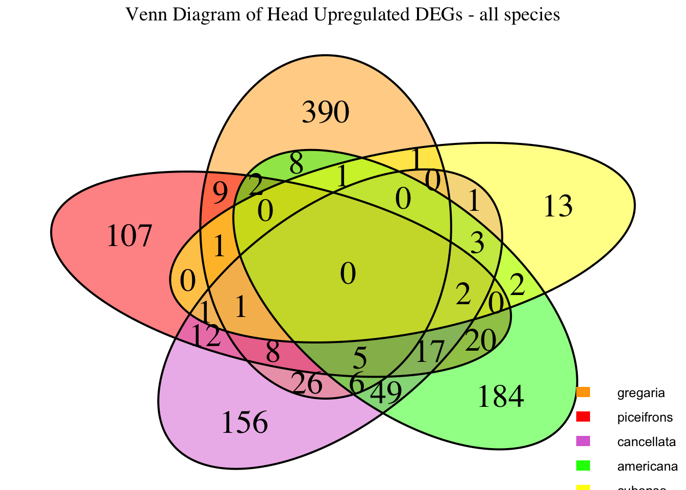
# Display the Venn diagram and datatable for head downregulated DEGs
display_venn_with_datatable(venn_data_down, "Venn Diagram of Head Downregulated DEGs - all species", allspecies_df)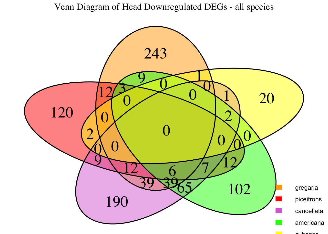
# Display the Venn diagram and datatable for all significant DEGs
display_venn_with_datatable(venn_data_all, "Venn Diagram of All Significant DEGs - all species", allspecies_df)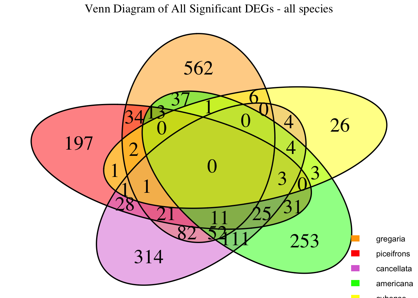
# Thorax
# Initialize an empty list to store DEG data
venn_data_allspecies_up <- list()
venn_data_allspecies_down <- list()
venn_data_allspecies_all <- list()

# Function to load DEGs for a given group of species for thorax
load_deg_data <- function(species_list) {
  degs_up <- list()
  degs_down <- list()
  degs_all <- list()

  for (species in allspecies) {
    thorax_file <- file.path(workDir, "DEG_results/Bulk_RNAseq/", paste0(species, "/Thorax/DESeq2_results_Thorax_", species,"_togregaria.csv"))

    thorax_data <- read.csv(thorax_file, stringsAsFactors = FALSE)

    # Check if data is empty and handle accordingly
    if (nrow(thorax_data) == 0) {
      message(paste("No data for species:", species))
      next  # Skip to the next species if there's no data
    }

    # Filter for significant DEGs (both upregulated and downregulated)
    thorax_up <- thorax_data %>%
      filter(padj < 0.05 & log2FoldChange >= 1) %>%
      select(GeneID = X)

    thorax_down <- thorax_data %>%
      filter(padj < 0.05 & log2FoldChange <= -1) %>%
      select(GeneID = X)

    all_deg <- thorax_data %>%
      filter(padj < 0.05 & abs(log2FoldChange) >= 1) %>%
      select(GeneID = X)

    # Store the DEGs in the list
    degs_up[[species]] <- thorax_up$GeneID
    degs_down[[species]] <- thorax_down$GeneID
    degs_all[[species]] <- all_deg$GeneID
  }

  return(list(up = degs_up, down = degs_down, all = degs_all))
}

# Load DEG data for Group 1 for thorax
venn_data_allspecies <- load_deg_data(allspecies)

# Prepare the data for the Venn diagrams
venn_data_up <- list(
  gregaria = venn_data_allspecies$up[["gregaria"]],
  piceifrons = venn_data_allspecies$up[["piceifrons"]],
  cancellata = venn_data_allspecies$up[["cancellata"]],
  americana = venn_data_allspecies$up[["americana"]],
  cubense = venn_data_allspecies$up[["cubense"]]
)

venn_data_down <- list(
  gregaria = venn_data_allspecies$down[["gregaria"]],
  piceifrons = venn_data_allspecies$down[["piceifrons"]],
  cancellata = venn_data_allspecies$down[["cancellata"]],
  americana = venn_data_allspecies$down[["americana"]],
  cubense = venn_data_allspecies$down[["cubense"]]
)

venn_data_all <- list(
  gregaria = venn_data_allspecies$all[["gregaria"]],
  piceifrons = venn_data_allspecies$all[["piceifrons"]],
  cancellata = venn_data_allspecies$all[["cancellata"]],
  americana = venn_data_allspecies$all[["americana"]],
  cubense = venn_data_allspecies$all[["cubense"]]
)

# Function to display Venn diagram and corresponding datatable
display_venn_with_datatable <- function(venn_data, title, allspecies_df) {
  # Calculate the overlapping genes
  overlap_genes <- Reduce(intersect, venn_data)

  # Create a data frame for the overlapping genes
  overlap_df <- data.frame(GeneID = overlap_genes)

  # Merge to get species information
  meta_brock_df <- merge(overlap_df, allspecies_df, by = "GeneID", all.x = TRUE)

  # Generate the Venn diagram
  venn_plot <- venn.diagram(
    x = venn_data,
    category.names = c("gregaria", "piceifrons", "cancellata","americana", "cubense"),
    filename = NULL,
    output = TRUE,
    fill = c("orange", "red", "orchid", "green", "yellow"),  # Set colors for the groups
    alpha = 0.5,
    cex = 2,
    cat.cex = 0,
    main = title,
    main.cex = 1.2
  )

  # Clear the current plotting area before drawing the Venn diagram
  grid.newpage()

  # Display the Venn diagram
  grid.draw(venn_plot)
    # Manually create a custom legend
    legend_labels <- c("gregaria", "piceifrons", "cancellata","americana", "cubense")
    legend_colors <- c("orange", "red", "orchid", "green", "yellow")

    # Positioning the legend lower on the right side of the plot
    legend_x <- unit(0.85, "npc")  # Adjust x position
    legend_y <- unit(0.2, "npc")    # Lower the legend vertically

    # Draw the legend
    for (i in 1:length(legend_labels)) {
        grid.rect(x = legend_x, y = legend_y - unit((i - 1) * 0.05, "npc"),
                  width = unit(0.02, "npc"), height = unit(0.02, "npc"),
                  gp = gpar(fill = legend_colors[i], col = NA))
        grid.text(label = legend_labels[i], x = legend_x + unit(0.05, "npc"),
                  y = legend_y - unit((i - 1) * 0.05, "npc"),
                  just = "left", gp = gpar(cex = 0.8))
    }
  # Display the merged overlapping genes table with datatable
  datatable(meta_brock_df, options = list(
      pageLength = 10,
      scrollX = TRUE,
      autoWidth = TRUE,
      searchHighlight = TRUE
  ),
  rownames = FALSE,
  escape = FALSE
  ) %>%
  formatStyle(
      'Species', target = 'cell',
      fontStyle = 'italic'
  ) %>%
  formatStyle(
      columns = names(meta_brock_df),
      target = 'row',
      color = styleEqual(c("red", "blue", "black"), c("red", "blue", "black")),
      fontWeight = styleEqual(c("bold", "normal"), c("bold", "normal")),
      backgroundColor = styleEqual(c("red", "blue", "black"), c("white", "white", "white"))
  )
}

# Display the Venn diagram and datatable for thorax upregulated DEGs
display_venn_with_datatable(venn_data_up, "Venn Diagram of Thorax Upregulated DEGs - all species", allspecies_df)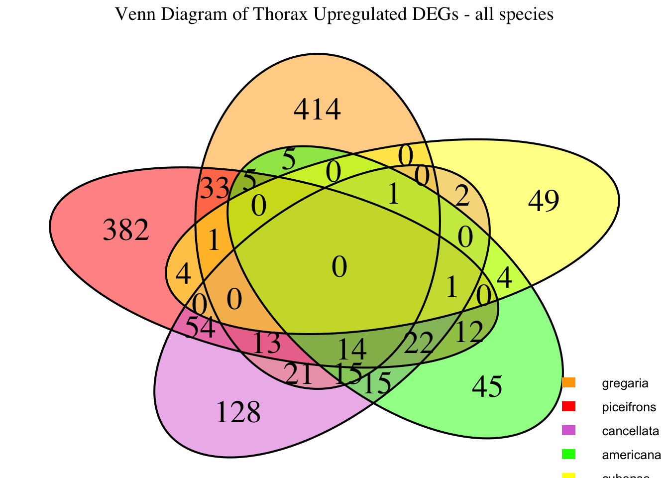
# Display the Venn diagram and datatable for head downregulated DEGs
display_venn_with_datatable(venn_data_down, "Venn Diagram of Thorax Downregulated DEGs - all species", allspecies_df)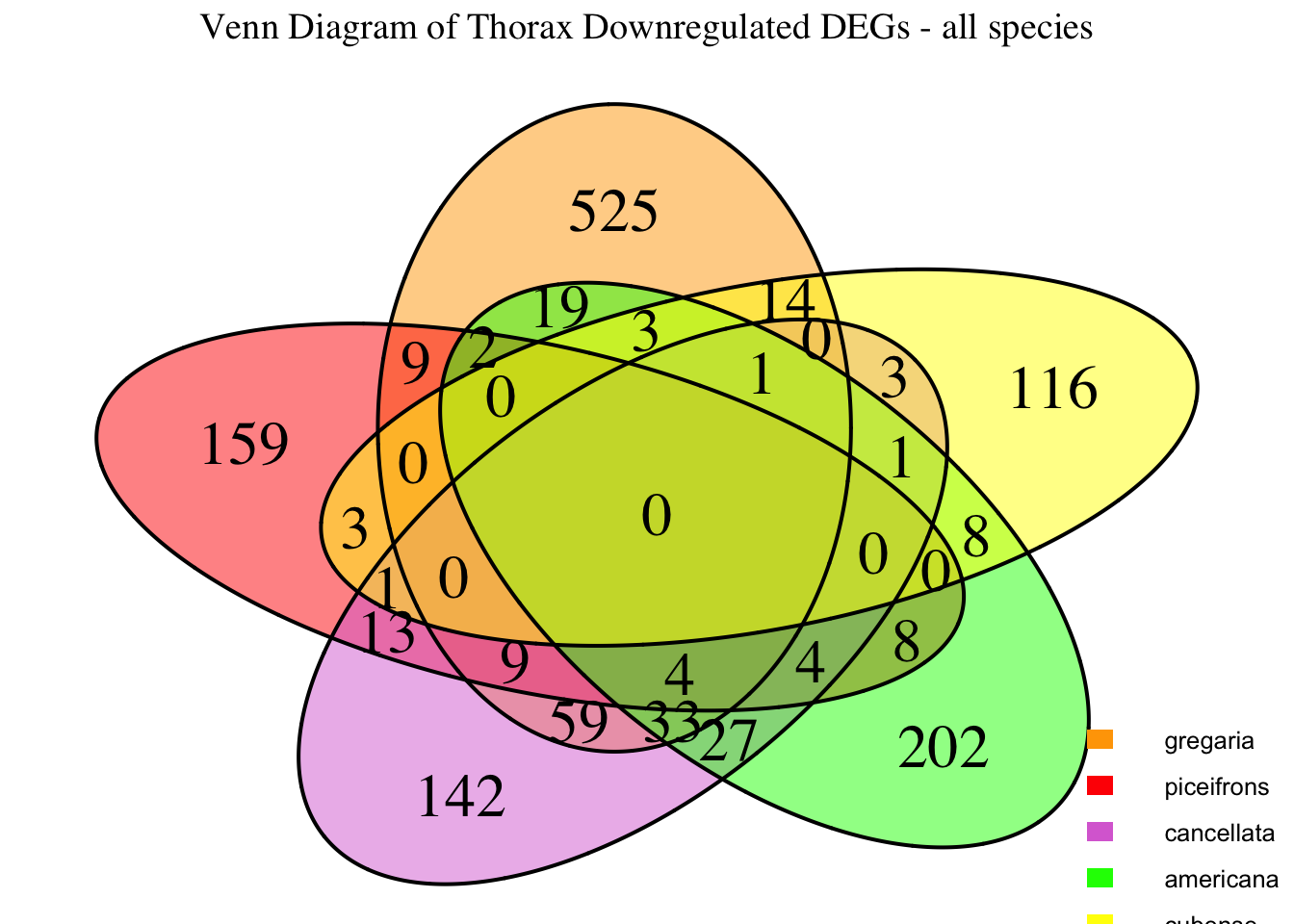
# Display the Venn diagram and datatable for all significant DEGs
display_venn_with_datatable(venn_data_all, "Venn Diagram of All Significant DEGs - all species", allspecies_df)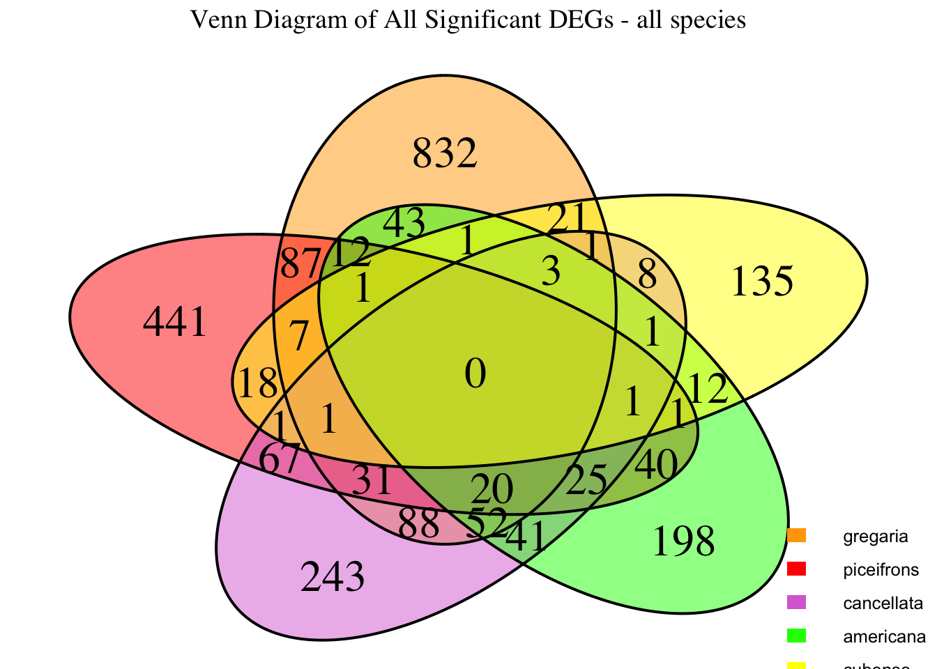
# Initialize an empty list to store heatmap data for each species
heatmap_list <- list()

# Loop through each species to process their data
for (species in species_list) {
  # Load DESeq2 results for head and thorax
  head_file <- file.path(workDir, "DEG_results/Bulk_RNAseq/", paste0(species, "/Head/DESeq2_results_Head_", species,"_togregaria.csv"))
  thorax_file <- file.path(workDir, "DEG_results/Bulk_RNAseq/", paste0(species, "/Thorax/DESeq2_results_Thorax_", species,"_togregaria.csv"))

  # Load the data
  head_data <- read.csv(head_file, stringsAsFactors = FALSE)
  thorax_data <- read.csv(thorax_file, stringsAsFactors = FALSE)

  # Check if data is empty and handle accordingly
  if (nrow(head_data) == 0 || nrow(thorax_data) == 0) {
    message(paste("No data for species:", species))
    next  # Skip to the next species if there's no data
  }

  # Filter for significant DEGs and select top 100 upregulated and downregulated genes for each tissue
  head_up <- head_data %>%
    filter(padj < 0.05 & log2FoldChange > 1) %>%
    arrange(desc(log2FoldChange)) %>%
    slice(1:500)

  head_down <- head_data %>%
    filter(padj < 0.05 & log2FoldChange < -1) %>%
    arrange(log2FoldChange) %>%
    slice(1:500)

  thorax_up <- thorax_data %>%
    filter(padj < 0.05 & log2FoldChange > 1) %>%
    arrange(desc(log2FoldChange)) %>%
    slice(1:500)

  thorax_down <- thorax_data %>%
    filter(padj < 0.05 & log2FoldChange < -1) %>%
    arrange(log2FoldChange) %>%
    slice(1:500)

  # Combine data and prepare for heatmap, adding the species column
  heatmap_data <- bind_rows(
    head_up %>% mutate(Tissue = "Head", Regulation = "Upregulated", Species = species),
    head_down %>% mutate(Tissue = "Head", Regulation = "Downregulated", Species = species),
    thorax_up %>% mutate(Tissue = "Thorax", Regulation = "Upregulated", Species = species),
    thorax_down %>% mutate(Tissue = "Thorax", Regulation = "Downregulated", Species = species)
  ) %>%
    select(GeneID, log2FoldChange, Tissue, Regulation, Species)


  # Append the heatmap data to the list
  heatmap_list[[species]] <- heatmap_data
}

# Combine all species data into a single dataframe for heatmap matrix preparation
final_heatmap_data <- bind_rows(heatmap_list)

# Check if final_heatmap_data is empty before proceeding
if (nrow(final_heatmap_data) == 0) {
  stop("No valid data available for heatmap generation.")
}

# Create heatmap matrix
# Aggregate log2FoldChange values correctly
heatmap_matrix <- final_heatmap_data %>%
  group_by(GeneID, Species, Tissue) %>%
  summarize(log2FoldChange = mean(log2FoldChange, na.rm = TRUE), .groups = "drop") %>%

  # Convert to wide format (no need for redundant grouping)
  pivot_wider(names_from = c(Species, Tissue), values_from = log2FoldChange, values_fill = 0) %>%

  # Ensure unique row names
  column_to_rownames("GeneID") %>%
  as.matrix()


custom_cyan_orange_palette <- colorRampPalette(c("cyan", "cyan2", "cyan3", "black", "orange3", "orange2", "orange"))(100)
custom_blue_red_palette <- colorRampPalette(c("blue3", "blue2", "blue1", "white", "red", "red2", "red3"))(100)

# Define color breaks to ensure **black = 0**
max_abs_lfc <- max(abs(heatmap_matrix), na.rm = TRUE)  # Get max absolute log2FoldChange
color_breaks <- seq(-max_abs_lfc, max_abs_lfc, length.out = 100)  # Symmetric scale

# Create first heatmap with blue-red gradient
pheatmap(
  heatmap_matrix,
  color = custom_blue_red_palette,
  breaks = color_breaks,
  cluster_rows = TRUE,
  cluster_cols = FALSE,
  show_rownames = FALSE,
  show_colnames = TRUE,
  fontsize_row = 6,
  fontsize_col = 10,
  main = "Heatmap of Gene Expression in Head and Thorax Tissue - STRATEGY 1"
)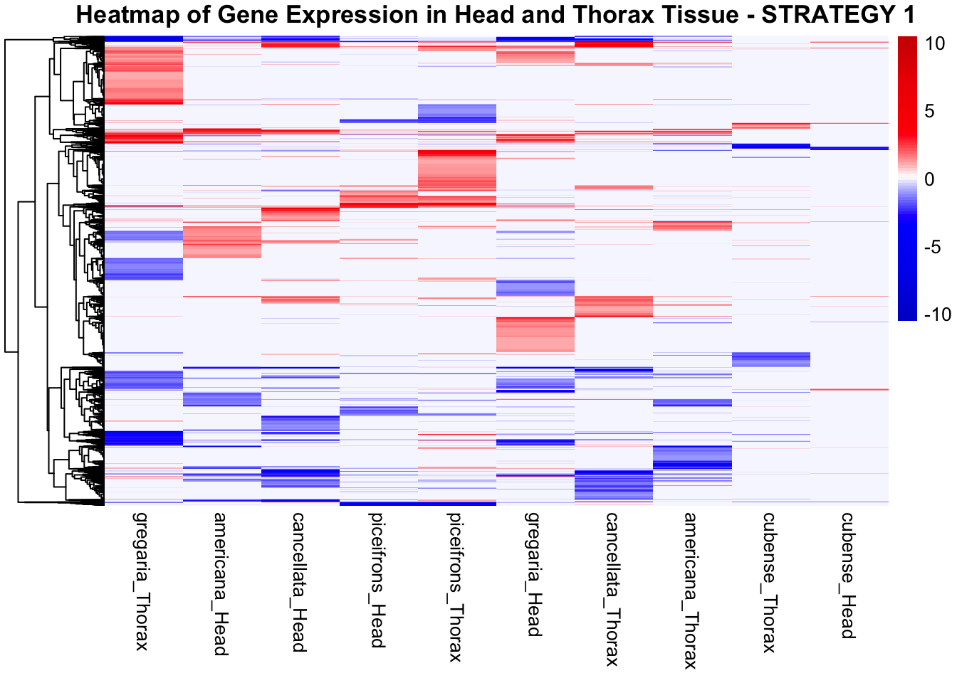
# Create second heatmap with cyan-black-orange gradient
pheatmap(
  heatmap_matrix,
  color = custom_cyan_orange_palette,
  breaks = color_breaks,
  cluster_rows = TRUE,
  cluster_cols = FALSE,
  show_rownames = FALSE,
  show_colnames = TRUE,
  fontsize_row = 6,
  fontsize_col = 10,
  main = "Heatmap of Gene Expression in Head and Thorax Tissue - STRATEGY 1"
)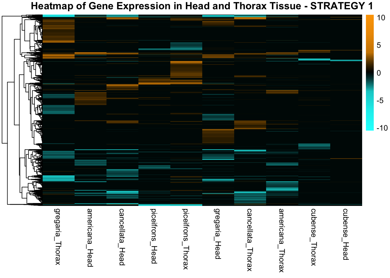
Head tissues
# Initialize an empty list to store heatmap data for each species
heatmap_list <- list()

# Loop through each species to process their data
for (species in species_list) {
  # Load DESeq2 results for head
  head_file <- file.path(workDir, "DEG_results/Bulk_RNAseq/", paste0(species, "/Head/DESeq2_results_Head_", species,"_togregaria.csv"))

  # Load the data
  head_data <- read.csv(head_file, stringsAsFactors = FALSE)

  # Check if data is empty and handle accordingly
  if (nrow(head_data) == 0) {
    message(paste("No data for species:", species))
    next  # Skip to the next species if there's no data
  }

  # Filter for significant DEGs and select top 100 upregulated and downregulated genes for each tissue
  head_up <- head_data %>%
    filter(padj < 0.05 & log2FoldChange > 1) %>%
    arrange(desc(log2FoldChange)) %>%
    slice(1:500)

  head_down <- head_data %>%
    filter(padj < 0.05 & log2FoldChange < -1) %>%
    arrange(log2FoldChange) %>%
    slice(1:500)

  # Combine data and prepare for heatmap, adding the species column
  heatmap_data <- bind_rows(
    head_up %>% mutate(Tissue = "Head", Regulation = "Upregulated", Species = species),
    head_down %>% mutate(Tissue = "Head", Regulation = "Downregulated", Species = species)
  ) %>%
    select(GeneID, log2FoldChange, Tissue, Regulation, Species)


  # Append the heatmap data to the list
  heatmap_list[[species]] <- heatmap_data
}

# Combine all species data
final_heatmap_data <- bind_rows(heatmap_list)

# Ensure all species are represented, even if they have no significant DEGs
for (species in species_order) {
    if (!species %in% unique(final_heatmap_data$Species)) {
        message(paste("Adding placeholder for missing species:", species))
        final_heatmap_data <- bind_rows(
            final_heatmap_data,
            data.frame(
                GeneID = "Unassigned",  # Placeholder GeneID
                log2FoldChange = 0,
                Tissue = "Head",
                Regulation = "None",
                Species = species
            )
        )
    }
}

# Ensure species order in the data
final_heatmap_data$Species <- factor(final_heatmap_data$Species, levels = species_order)

# Create heatmap matrix (Thorax only)
heatmap_matrix <- final_heatmap_data %>%
  group_by(GeneID, Species) %>%
  summarize(log2FoldChange = mean(log2FoldChange, na.rm = TRUE), .groups = "drop") %>%
  pivot_wider(names_from = Species, values_from = log2FoldChange, values_fill = 0) %>%
  column_to_rownames("GeneID") %>%
  as.matrix()

# Explicitly reorder the columns in heatmap_matrix
heatmap_matrix <- heatmap_matrix[, species_order, drop = FALSE]

# Define color palettes
custom_cyan_orange_palette <- colorRampPalette(c("cyan", "cyan2", "cyan3", "black", "orange3", "orange2", "orange"))(100)
custom_blue_red_palette <- colorRampPalette(c("blue3", "blue2", "blue1", "white", "red", "red2", "red3"))(100)

# Define color breaks to ensure **black = 0**
max_abs_lfc <- max(abs(heatmap_matrix), na.rm = TRUE)  # Get max absolute log2FoldChange
color_breaks <- seq(-max_abs_lfc, max_abs_lfc, length.out = 100)  # Symmetric scale

# Create first heatmap with blue-red gradient
pheatmap(
  heatmap_matrix,
  color = custom_blue_red_palette,
  breaks = color_breaks,
  cluster_rows = TRUE,
  cluster_cols = FALSE,
  show_rownames = FALSE,
  show_colnames = TRUE,
  fontsize_row = 6,
  fontsize_col = 10,
  main = "Heatmap of Gene Expression in Head Tissue - STRATEGY 1"
)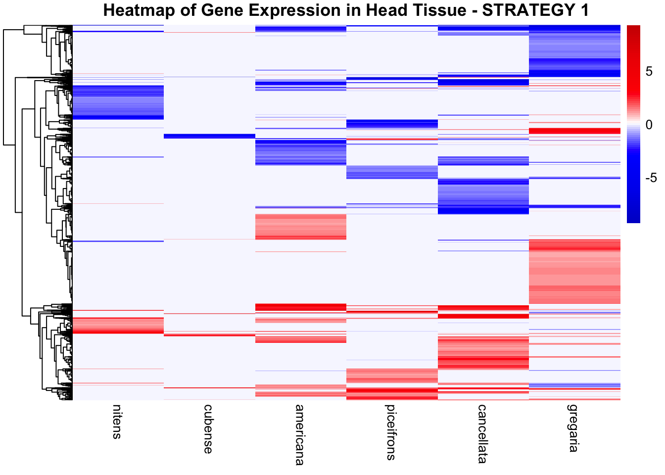
# Create second heatmap with cyan-black-orange gradient
pheatmap(
  heatmap_matrix,
  color = custom_cyan_orange_palette,
  breaks = color_breaks,
  cluster_rows = TRUE,
  cluster_cols = FALSE,
  show_rownames = FALSE,
  show_colnames = TRUE,
  fontsize_row = 6,
  fontsize_col = 10,
  main = "Heatmap of Gene Expression in Head Tissue - STRATEGY 1"
)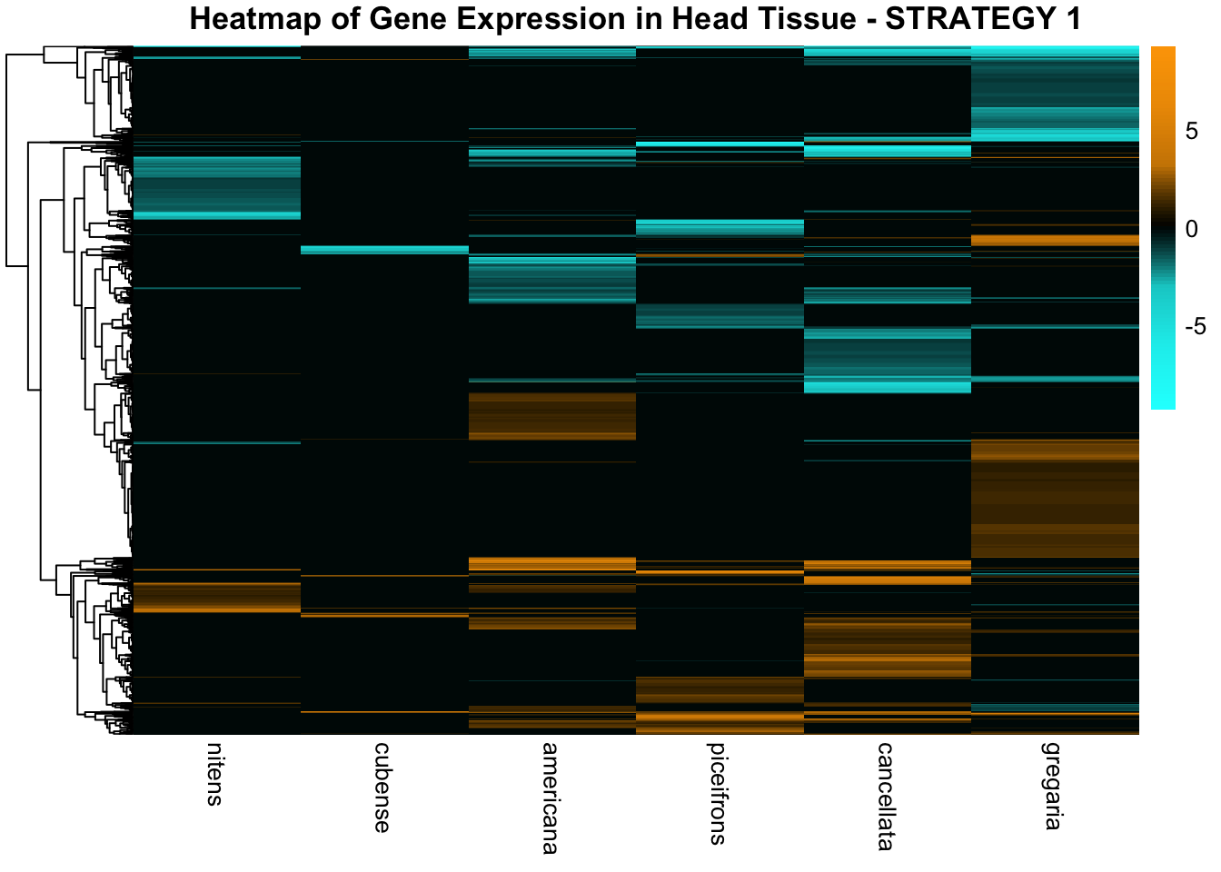
Thorax tissues
# Define species order explicitly to ensure consistency
species_order <- c("nitens", "cubense", "americana", "piceifrons", "cancellata", "gregaria")

# Initialize an empty list to store heatmap data
heatmap_list <- list()

# Loop through each species to process their Thorax data
for (species in species_order) {
  message(paste("Processing species:", species))

  # Define file path for Thorax
  thorax_file <- file.path(workDir, "DEG_results/Bulk_RNAseq/", paste0(species, "/Thorax/DESeq2_results_Thorax_", species,"_togregaria.csv"))

  # Check if file exists before loading
  if (!file.exists(thorax_file)) {
    message(paste("Missing Thorax file for:", species, "- Assigning empty dataset"))
    thorax_data <- data.frame(GeneID = character(), padj = numeric(), log2FoldChange = numeric(), stringsAsFactors = FALSE)
  } else {
    thorax_data <- tryCatch(read.csv(thorax_file, stringsAsFactors = FALSE), error = function(e) data.frame())
  }

  # Ensure GeneID column exists
  if (!"GeneID" %in% colnames(thorax_data) && "X" %in% colnames(thorax_data)) {
    colnames(thorax_data)[colnames(thorax_data) == "X"] <- "GeneID"
  }

  # Convert GeneID to character
  thorax_data$GeneID <- as.character(thorax_data$GeneID)

  # If no significant DEGs are found, ensure the structure is correct
  if (nrow(thorax_data) == 0) {
    message(paste("No significant Thorax DEGs for:", species, "- Assigning placeholder values"))
    thorax_data <- data.frame(
      GeneID = "Unassigned",
      log2FoldChange = 0,
      Tissue = "Thorax",
      Regulation = "None",
      Species = species
    )
  } else {
    # Filter for significant DEGs and select top 500 upregulated and downregulated genes
    thorax_up <- thorax_data %>%
      filter(padj < 0.05 & log2FoldChange > 1) %>%
      arrange(desc(log2FoldChange)) %>%
      slice(1:500)

    thorax_down <- thorax_data %>%
      filter(padj < 0.05 & log2FoldChange < -1) %>%
      arrange(log2FoldChange) %>%
      slice(1:500)

    # Combine data and prepare for heatmap
    thorax_data <- bind_rows(
      thorax_up %>% mutate(Tissue = "Thorax", Regulation = "Upregulated", Species = species),
      thorax_down %>% mutate(Tissue = "Thorax", Regulation = "Downregulated", Species = species)
    ) %>%
      select(GeneID, log2FoldChange, Tissue, Regulation, Species)
  }

  # Append to heatmap list, ensuring species is represented
  heatmap_list[[species]] <- thorax_data
}

# Combine all species data
final_heatmap_data <- bind_rows(heatmap_list)

# Ensure all species are represented, even if they have no significant DEGs
for (species in species_order) {
    if (!species %in% unique(final_heatmap_data$Species)) {
        message(paste("Adding placeholder for missing species:", species))
        final_heatmap_data <- bind_rows(
            final_heatmap_data,
            data.frame(
                GeneID = "Unassigned",  # Placeholder GeneID
                log2FoldChange = 0,
                Tissue = "Thorax",
                Regulation = "None",
                Species = species
            )
        )
    }
}

# Ensure species order in the data
final_heatmap_data$Species <- factor(final_heatmap_data$Species, levels = species_order)

# Create heatmap matrix (Thorax only)
heatmap_matrix <- final_heatmap_data %>%
  group_by(GeneID, Species) %>%
  summarize(log2FoldChange = mean(log2FoldChange, na.rm = TRUE), .groups = "drop") %>%
  pivot_wider(names_from = Species, values_from = log2FoldChange, values_fill = 0) %>%
  column_to_rownames("GeneID") %>%
  as.matrix()

# Explicitly reorder the columns in heatmap_matrix
heatmap_matrix <- heatmap_matrix[, species_order, drop = FALSE]

# Define color palettes
custom_cyan_orange_palette <- colorRampPalette(c("cyan", "cyan2", "cyan3", "black", "orange3", "orange2", "orange"))(100)
custom_blue_red_palette <- colorRampPalette(c("blue3", "blue2", "blue1", "white", "red", "red2", "red3"))(100)

# Define color breaks
max_abs_lfc <- max(abs(heatmap_matrix), na.rm = TRUE)
color_breaks <- seq(-max_abs_lfc, max_abs_lfc, length.out = 100)

# Generate heatmaps (Only thorax)
pheatmap(
  heatmap_matrix,
  color = custom_blue_red_palette,
  breaks = color_breaks,
  cluster_rows = TRUE,
  cluster_cols = FALSE,
  show_rownames = FALSE,
  show_colnames = TRUE,
  fontsize_row = 6,
  fontsize_col = 10,
  main = "Heatmap of GeneID Expression in Thorax Tissue - STRATEGY 1"
)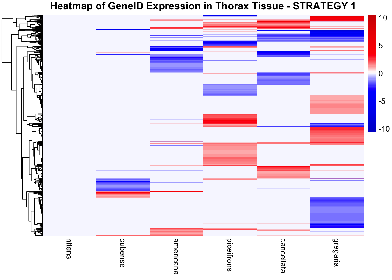
pheatmap(
  heatmap_matrix,
  color = custom_cyan_orange_palette,
  breaks = color_breaks,
  cluster_rows = TRUE,
  cluster_cols = FALSE,
  show_rownames = FALSE,
  show_colnames = TRUE,
  fontsize_row = 6,
  fontsize_col = 10,
  main = "Heatmap of GeneID Expression in Thorax Tissue - STRATEGY 1"
)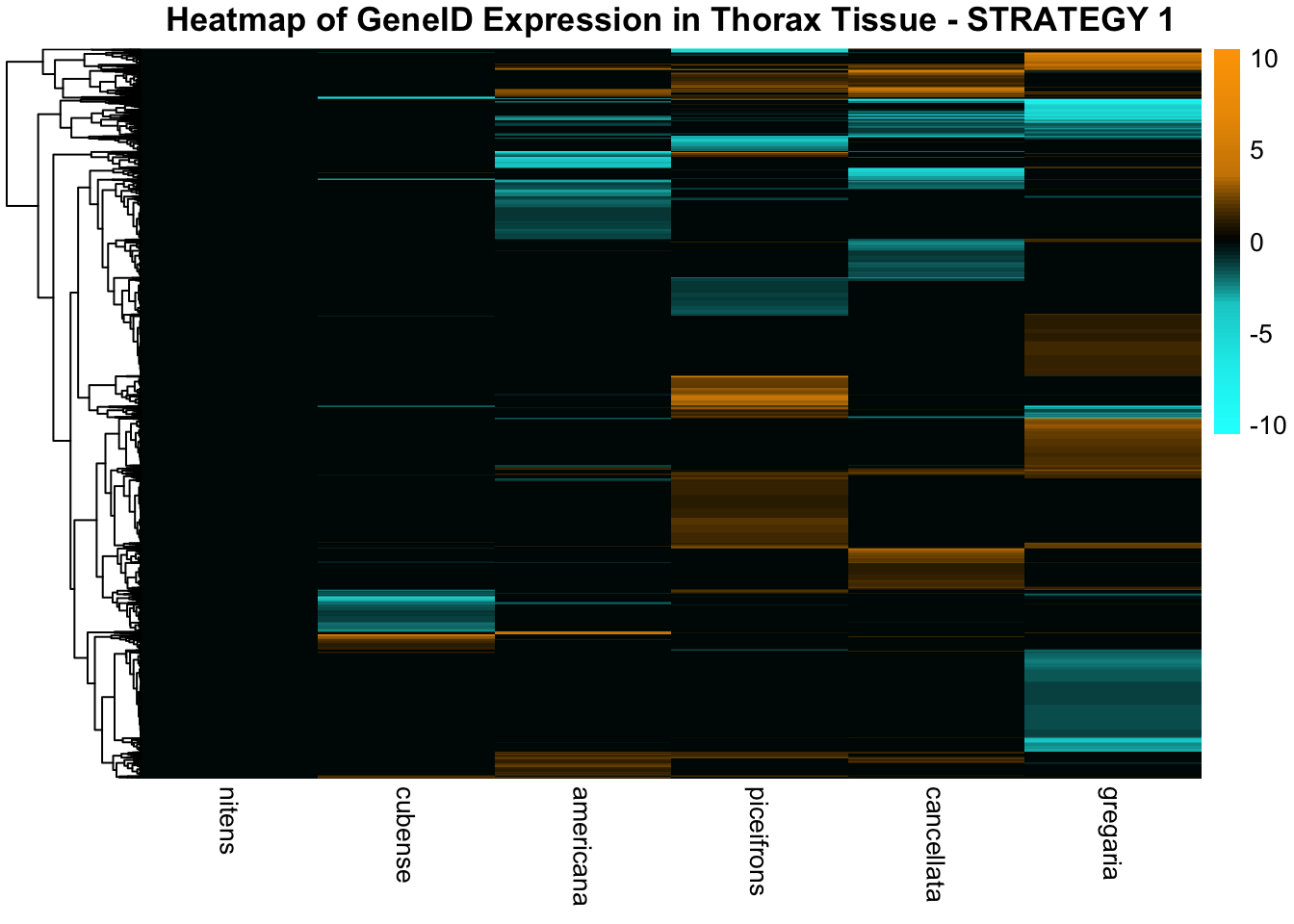
All species
Combined tissues
# Define the species list
allspecies <- c("nitens", "cubense", "americana", "piceifrons", "cancellata", "gregaria")

# Function to load DEGs for all species
load_species_deg_data <- function(tissue) {
  degs_up <- list()
  degs_down <- list()
  degs_all <- list()

  for (species in allspecies) {
    deg_file <- file.path(workDir, "DEG_results/Bulk_RNAseq", paste0(species, "/", tissue, "/DESeq2_results_", tissue, "_", species, "_togregaria.csv"))

    if (!file.exists(deg_file)) {
      message(paste("File missing for species:", species))
      next  # Skip if the file doesn't exist
    }

    deg_data <- read.csv(deg_file, stringsAsFactors = FALSE)

    # Check if data is empty
    if (nrow(deg_data) == 0) {
      message(paste("No data for species:", species))
      next
    }

    # Select significant DEGs (Up, Down, All)
    degs_up[[species]] <- deg_data %>%
      filter(padj < 0.05 & log2FoldChange >= 1) %>%
      pull(X)  # Ensure GeneID is extracted properly

    degs_down[[species]] <- deg_data %>%
      filter(padj < 0.05 & log2FoldChange <= -1) %>%
      pull(X)

    degs_all[[species]] <- deg_data %>%
      filter(padj < 0.05 & abs(log2FoldChange) >= 1) %>%
      pull(X)
  }

  return(list(up = degs_up, down = degs_down, all = degs_all))
}

# Load DEG data for head and thorax
venn_data_head <- load_species_deg_data("Head")
venn_data_thorax <- load_species_deg_data("Thorax")

# Function to visualize Venn diagram using ggVennDiagram
display_ggvenn_plot <- function(venn_data, title) {
  gg_venn <- ggVennDiagram(venn_data, label_alpha = 0, edge_lty = "dashed") +
    scale_fill_gradient(low = "lightblue", high = "darkblue") +
    labs(title = title) +
    theme_minimal(base_size = 14)

  return(gg_venn)
}

# **Generate Venn diagrams**
ggvenn_head_up <- display_ggvenn_plot(venn_data_head$up, "Venn Diagram of Head Upregulated DEGs - All Species")
ggvenn_head_down <- display_ggvenn_plot(venn_data_head$down, "Venn Diagram of Head Downregulated DEGs - All Species")
ggvenn_head_all <- display_ggvenn_plot(venn_data_head$all, "Venn Diagram of All Significant DEGs (Head) - All Species")

ggvenn_thorax_up <- display_ggvenn_plot(venn_data_thorax$up, "Venn Diagram of Thorax Upregulated DEGs - All Species")
ggvenn_thorax_down <- display_ggvenn_plot(venn_data_thorax$down, "Venn Diagram of Thorax Downregulated DEGs - All Species")
ggvenn_thorax_all <- display_ggvenn_plot(venn_data_thorax$all, "Venn Diagram of All Significant DEGs (Thorax) - All Species")


####### Upset plots

load_deseq2_upset_data <- function(tissue) {
  # Initialize an empty list to store gene sets per species
  species_deg_list <- list()

  for (species in allspecies) {
    # Construct the correct file path
    deg_file <- file.path(workDir, "DEG_results/Bulk_RNAseq", species, tissue,
                          paste0("DESeq2_results_", tissue, "_", species, "_togregaria.csv"))

    # Skip if file does not exist
    if (!file.exists(deg_file)) {
      message(paste("File missing for species:", species))
      next
    }

    # Load the DESeq2 results file
    deseq_data <- read.csv(deg_file, stringsAsFactors = FALSE)

    # Check for the correct column name
    if (!"GeneID" %in% colnames(deseq_data)) {
      if ("X" %in% colnames(deseq_data)) {
        colnames(deseq_data)[colnames(deseq_data) == "X"] <- "GeneID"
      } else {
        stop(paste("Error: No 'GeneID' or 'X' column found in", deg_file))
      }
    }

    # Filter for significant DEGs
    significant_genes <- deseq_data %>%
      filter(padj < 0.05 & abs(log2FoldChange) >= 1) %>%
      pull(GeneID)

    # Store the gene list for the species
    species_deg_list[[species]] <- significant_genes
  }

  # Create a binary matrix for UpSet plot
  all_genes <- unique(unlist(species_deg_list))  # Collect all unique DEGs
  upset_data <- data.frame(GeneID = all_genes)

  for (species in allspecies) {
    upset_data[[species]] <- as.integer(all_genes %in% species_deg_list[[species]])
  }

  return(upset_data)
}

upset_data_head <- load_deseq2_upset_data("Head")
upset_data_thorax <- load_deseq2_upset_data("Thorax")


###############

display_upset_plot <- function(upset_data, title) {
    upset_plot <- upset(
        upset_data,
        allspecies,
                queries = list(
            upset_query(
                intersect = c('gregaria', 'cancellata'),
                color = 'orange',
                fill = 'orange',
                only_components = c('intersections_matrix', 'Intersection size')
            ),
            upset_query(
                intersect = c('gregaria', 'piceifrons'),
                color = 'orange',
                fill = 'orange',
                only_components = c('intersections_matrix', 'Intersection size')
            ),
            upset_query(
                intersect = c('cancellata', 'piceifrons'),
                color = 'orange',
                fill = 'orange',
                only_components = c('intersections_matrix', 'Intersection size')
            ),
            upset_query(
                intersect = c('gregaria', 'piceifrons', 'cancellata'),
                color = 'darkred',
                fill = 'darkred',
                only_components = c('intersections_matrix', 'Intersection size')
            ),
            upset_query(
                intersect = c('gregaria', 'piceifrons', 'cancellata', 'americana'),
                color = 'purple',
                fill = 'purple',
                only_components = c('intersections_matrix', 'Intersection size')
            ),
            upset_query(set = 'gregaria', fill = 'darkred'),
            upset_query(set = 'piceifrons', fill = 'darkred'),
            upset_query(set = 'cancellata', fill = 'darkred'),
            upset_query(set = 'americana', fill = 'black'),
            upset_query(set = 'cubense', fill = 'black'),
            upset_query(set = 'nitens', fill = 'black')
        ),
        sort_sets = FALSE,
        base_annotations = list(
            'Intersection size' = intersection_size(counts = FALSE) +
                ylab('# DEGs in intersection') +
                scale_y_continuous(expand = expansion(mult = c(0, 0.05)))
        ),
        intersection_matrix(
            geom = geom_point(
                shape = 'circle',
                size = 4
            ),
            segment = geom_segment(
                linetype = 'solid',
                size = 3
            ),
            outline_color = list(
                active = 'black',
                inactive = 'grey80'
            )
        ) +
        theme(
            axis.text.x = element_text(face = "bold", size = 12, angle = 45, hjust = 1, color = "darkblue"),
            axis.text.y = element_text(face = "italic", size = 12, color = "darkred"),
            axis.ticks.length = unit(0.25, "cm")
        ),
        set_sizes = upset_set_size(
            geom = geom_bar(width = 0.8),
            position = 'right'
        ) +
        ylab('# DEGs per species') +
        theme(
            axis.line.x = element_line(colour = 'black'),
            axis.ticks.x = element_line()
        ),
        stripes = upset_stripes(
            geom = geom_segment(size = 12),
            colors = c('grey95', 'white')
        ),
    ) +
    theme_minimal() +
    theme(
        panel.grid.major = element_blank(),
        panel.grid.minor = element_blank(),
        axis.line = element_line(colour = 'black'),
        text = element_text(size = 14),
        axis.text.x = element_text(face = "italic"),
        plot.title = element_text(hjust = 0.5, face = "bold", size = 16)
    ) +
    ggtitle(title)

    return(upset_plot)
}


upset_head <- display_upset_plot(upset_data_head, "Intersection from Head")
ggvenn_head_all; print(upset_head)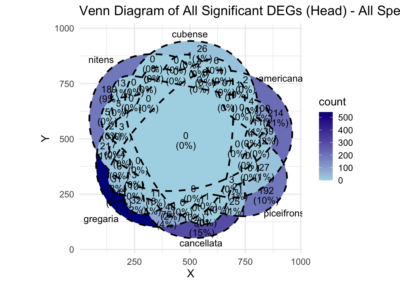
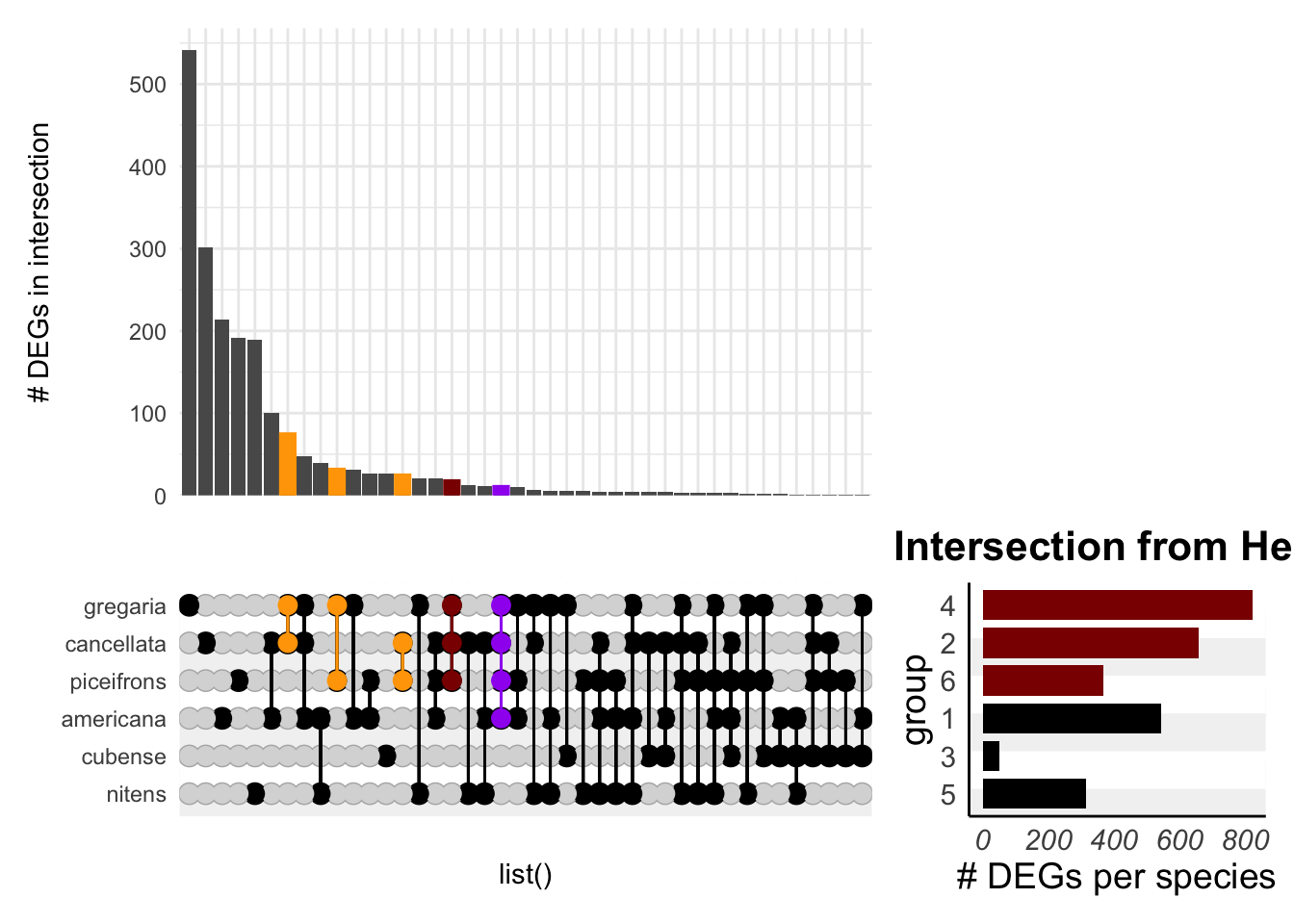
upset_thorax <- display_upset_plot(upset_data_thorax, "Intersection from Thorax")
ggvenn_thorax_all; print(upset_thorax)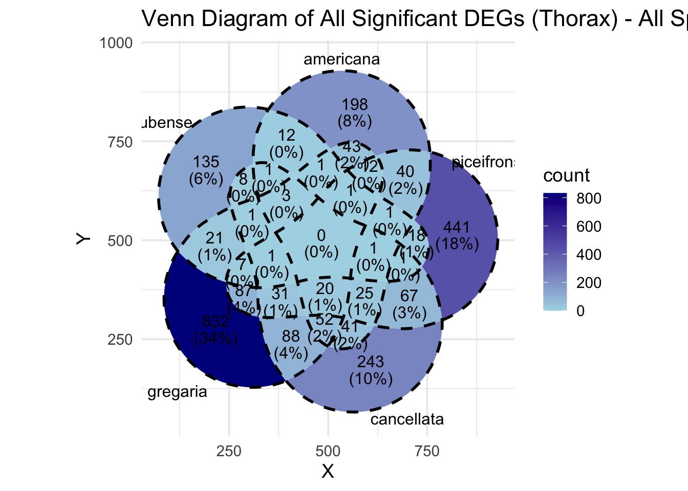
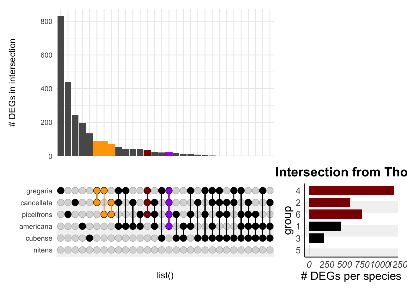
# Function to extract GeneIDs for a specific intersection
extract_geneids_from_intersection <- function(upset_data, selected_species) {
    # Ensure the input species exist in the dataset
    selected_species <- intersect(selected_species, colnames(upset_data))

    # Select rows where all selected species have '1' (present in the intersection)
    intersecting_genes <- upset_data[rowSums(upset_data[selected_species]) == length(selected_species), ]

    # Return only the GeneIDs as a DataFrame
    return(data.frame(GeneID = intersecting_genes$GeneID))
}

# **Shared GeneIDs among Gregaria, Cancellata, and Piceifrons (Head)**
shared_geneids_head <- extract_geneids_from_intersection(upset_data_head, c("gregaria", "cancellata", "piceifrons"))

kable(shared_geneids_head, col.names = c("Head: shared genes among all locusts")) %>%
kable_styling(bootstrap_options = c("striped", "hover"))| Head: shared genes among all locusts |
|---|
| LOC126334877 |
| LOC126335646 |
| LOC126282005 |
| LOC126335148 |
| LOC126353995 |
| LOC126269449 |
| LOC126268224 |
| LOC126272473 |
| LOC126271867 |
| LOC126272311 |
| LOC126282249 |
| LOC126282270 |
| LOC126284250 |
| LOC126293182 |
| LOC126298855 |
| LOC126274577 |
| LOC126336183 |
| LOC126353962 |
| LOC126354941 |
| LOC126355774 |
| LOC126266785 |
| LOC126268096 |
| LOC126273126 |
| LOC126272290 |
| LOC126272573 |
| LOC126272572 |
| LOC126272125 |
| LOC126281584 |
| LOC126281827 |
| LOC126284303 |
| LOC126284563 |
| LOC126291853 |
| LOC126292013 |
# **Shared GeneIDs among Gregaria, Cancellata, Piceifrons, and Americana (Head)**
shared_geneids_head_americana <- extract_geneids_from_intersection(upset_data_head, c("gregaria", "cancellata", "piceifrons", "americana"))

kable(shared_geneids_head_americana, col.names = c("Head: shared genes among all locusts + americana")) %>%
kable_styling(bootstrap_options = c("striped", "hover"))| Head: shared genes among all locusts + americana |
|---|
| LOC126353995 |
| LOC126269449 |
| LOC126268224 |
| LOC126272473 |
| LOC126271867 |
| LOC126272311 |
| LOC126282249 |
| LOC126282270 |
| LOC126284250 |
| LOC126293182 |
| LOC126298855 |
# **Shared GeneIDs among Gregaria, Cancellata, and Piceifrons (Thorax)**
shared_geneids_thorax <- extract_geneids_from_intersection(upset_data_thorax, c("gregaria", "cancellata", "piceifrons"))

kable(shared_geneids_thorax, col.names = c("Thorax: shared genes among all locusts")) %>%
kable_styling(bootstrap_options = c("striped", "hover"))| Thorax: shared genes among all locusts |
|---|
| LOC126284484 |
| LOC126284981 |
| LOC126334921 |
| LOC126344463 |
| LOC126345116 |
| LOC126269449 |
| LOC126336408 |
| LOC126336415 |
| LOC126336987 |
| LOC126353822 |
| LOC126355556 |
| LOC126355925 |
| LOC126267550 |
| LOC126272787 |
| LOC126272949 |
| LOC126273038 |
| LOC126282270 |
| LOC126284671 |
| LOC126284704 |
| LOC126291753 |
| LOC126298650 |
| LOC126280525 |
| LOC126334877 |
| LOC126335646 |
| LOC126335750 |
| LOC126337060 |
| LOC126334545 |
| LOC126335148 |
| LOC126335450 |
| LOC126356355 |
| LOC126353960 |
| LOC126353962 |
| LOC126355499 |
| LOC126267274 |
| LOC126273126 |
| LOC126273131 |
| LOC126273132 |
| LOC126273129 |
| LOC126271867 |
| LOC126272290 |
| LOC126272573 |
| LOC126272892 |
| LOC126277894 |
| LOC126282005 |
| LOC126281827 |
| LOC126281298 |
| LOC126284240 |
| LOC126291853 |
| LOC126291616 |
| LOC126293406 |
| LOC126293648 |
| LOC126294994 |
# **Shared GeneIDs among Gregaria, Cancellata, Piceifrons, and Americana (Thorax)**
shared_geneids_thorax_americana <- extract_geneids_from_intersection(upset_data_thorax, c("gregaria", "cancellata", "piceifrons", "americana"))

kable(shared_geneids_thorax_americana, col.names = c("Thorax: shared genes among all locusts + americana")) %>%
kable_styling(bootstrap_options = c("striped", "hover"))| Thorax: shared genes among all locusts + americana |
|---|
| LOC126284981 |
| LOC126334921 |
| LOC126344463 |
| LOC126345116 |
| LOC126269449 |
| LOC126336408 |
| LOC126336415 |
| LOC126336987 |
| LOC126353822 |
| LOC126355556 |
| LOC126355925 |
| LOC126267550 |
| LOC126272787 |
| LOC126272949 |
| LOC126273038 |
| LOC126282270 |
| LOC126284671 |
| LOC126284704 |
| LOC126291753 |
| LOC126298650 |
# **Shared GeneIDs among Gregaria and Piceifrons (Head)**
shared_geneids_head_piceifrons_gregaria <- extract_geneids_from_intersection(upset_data_head, c("gregaria", "piceifrons"))

kable(shared_geneids_head_piceifrons_gregaria, col.names = c("Head: shared genes between gregaria & piceifrons")) %>%
kable_styling(bootstrap_options = c("striped", "hover"))| Head: shared genes between gregaria & piceifrons |
|---|
| LOC126312183 |
| LOC126334877 |
| LOC126335646 |
| LOC126356328 |
| LOC126282005 |
| LOC126281697 |
| LOC126291991 |
| LOC126298049 |
| LOC126346425 |
| LOC126335605 |
| LOC126335148 |
| LOC126353995 |
| LOC126269449 |
| LOC126336415 |
| LOC126334614 |
| LOC126335450 |
| LOC126335543 |
| LOC126354368 |
| LOC126355772 |
| LOC126268224 |
| LOC126272473 |
| LOC126271867 |
| LOC126271906 |
| LOC126272311 |
| LOC126278164 |
| LOC126278162 |
| LOC126282249 |
| LOC126282250 |
| LOC126282270 |
| LOC126284250 |
| LOC126293182 |
| LOC126298855 |
| LOC126325647 |
| LOC126355923 |
| LOC126360279 |
| LOC126274561 |
| LOC126274577 |
| LOC126274545 |
| LOC126281377 |
| LOC126336183 |
| LOC126335847 |
| LOC126332220 |
| LOC126335083 |
| LOC126353961 |
| LOC126353962 |
| LOC126354707 |
| LOC126354240 |
| LOC126355817 |
| LOC126354934 |
| LOC126354935 |
| LOC126354941 |
| LOC126355774 |
| LOC126355859 |
| LOC126365802 |
| LOC126266785 |
| LOC126268096 |
| LOC126267730 |
| LOC126268046 |
| LOC126273126 |
| LOC126272290 |
| LOC126272573 |
| LOC126272572 |
| LOC126271905 |
| LOC126272598 |
| LOC126272125 |
| LOC126277896 |
| LOC126277898 |
| LOC126278583 |
| LOC126281584 |
| LOC126282247 |
| LOC126281222 |
| LOC126281273 |
| LOC126281827 |
| LOC126282035 |
| LOC126284303 |
| LOC126284563 |
| LOC126284500 |
| LOC126291853 |
| LOC126292013 |
| LOC126293425 |
| LOC126295132 |
| LOC126295147 |
# **Shared GeneIDs among Piceifrons and Cancellata (Head)**
shared_geneids_head_piceifrons_cancellata <- extract_geneids_from_intersection(upset_data_head, c("piceifrons", "cancellata"))

kable(shared_geneids_head_piceifrons_cancellata, col.names = c("Head: shared genes between piceifrons & Cancellata")) %>%
kable_styling(bootstrap_options = c("striped", "hover"))| Head: shared genes between piceifrons & Cancellata |
|---|
| LOC126334877 |
| LOC126335646 |
| LOC126335513 |
| LOC126354343 |
| LOC126267269 |
| LOC126272552 |
| LOC126272571 |
| LOC126272901 |
| LOC126282005 |
| LOC126297489 |
| LOC126336417 |
| LOC126334880 |
| LOC126336207 |
| LOC126335148 |
| LOC126272684 |
| LOC126334921 |
| LOC126349427 |
| LOC126353995 |
| LOC126269449 |
| LOC126283252 |
| LOC126323134 |
| LOC126334992 |
| LOC126354154 |
| LOC126354567 |
| LOC126355490 |
| LOC126355258 |
| LOC126355925 |
| LOC126268219 |
| LOC126268224 |
| LOC126266629 |
| LOC126267420 |
| LOC126267952 |
| LOC126272473 |
| LOC126272886 |
| LOC126273222 |
| LOC126271867 |
| LOC126272311 |
| LOC126272289 |
| LOC126282249 |
| LOC126282270 |
| LOC126285392 |
| LOC126284250 |
| LOC126284858 |
| LOC126293182 |
| LOC126293510 |
| LOC126295330 |
| LOC126298855 |
| LOC126268233 |
| LOC126274577 |
| LOC126336491 |
| LOC126323151 |
| LOC126336183 |
| LOC126354441 |
| LOC126354172 |
| LOC126353959 |
| LOC126353962 |
| LOC126354941 |
| LOC126355774 |
| LOC126267280 |
| LOC126365811 |
| LOC126266785 |
| LOC126365781 |
| LOC126268096 |
| LOC126365968 |
| LOC126271859 |
| LOC126273126 |
| LOC126272290 |
| LOC126272573 |
| LOC126272572 |
| LOC126272125 |
| LOC126278646 |
| LOC126278158 |
| LOC126282076 |
| LOC126281584 |
| LOC126281482 |
| LOC126281687 |
| LOC126281827 |
| LOC126282264 |
| LOC126284446 |
| LOC126284704 |
| LOC126284303 |
| LOC126284428 |
| LOC126284563 |
| LOC126284300 |
| LOC126291853 |
| LOC126292013 |
| LOC126294994 |
| LOC126295256 |
| LOC126299329 |
| LOC126302631 |
# **Shared GeneIDs among Cancellata and Gregaria (Head)**
shared_geneids_head_cancellata_gregaria <- extract_geneids_from_intersection(upset_data_head, c("cancellata", "gregaria"))

kable(shared_geneids_head_cancellata_gregaria, col.names = c("Head: shared genes between cancellata & gregaria")) %>%
kable_styling(bootstrap_options = c("striped", "hover"))| Head: shared genes between cancellata & gregaria |
|---|
| LOC126362949 |
| LOC126334876 |
| LOC126334878 |
| LOC126334877 |
| LOC126335646 |
| LOC126332740 |
| LOC126272892 |
| LOC126272891 |
| LOC126272825 |
| LOC126282005 |
| LOC126284695 |
| LOC126295127 |
| LOC126294990 |
| LOC126297738 |
| LOC126335148 |
| LOC126335221 |
| LOC126353995 |
| LOC126269449 |
| LOC126279173 |
| LOC126336408 |
| LOC126336445 |
| LOC126335660 |
| LOC126336602 |
| LOC126336884 |
| LOC126325085 |
| LOC126336469 |
| LOC126353822 |
| LOC126356046 |
| LOC126356355 |
| LOC126356365 |
| LOC126355429 |
| LOC126355428 |
| LOC126355446 |
| LOC126355498 |
| LOC126355523 |
| LOC126355518 |
| LOC126355524 |
| LOC126355525 |
| LOC126355499 |
| LOC126355503 |
| LOC126355507 |
| LOC126355515 |
| LOC126355693 |
| LOC126355555 |
| LOC126354675 |
| LOC126354383 |
| LOC126355587 |
| LOC126268224 |
| LOC126267553 |
| LOC126267148 |
| LOC126365815 |
| LOC126267904 |
| LOC126272473 |
| LOC126272787 |
| LOC126271867 |
| LOC126271903 |
| LOC126273012 |
| LOC126272311 |
| LOC126271954 |
| LOC126282249 |
| LOC126282270 |
| LOC126281236 |
| LOC126284276 |
| LOC126284565 |
| LOC126284785 |
| LOC126284250 |
| LOC126284312 |
| LOC126291970 |
| LOC126291614 |
| LOC126293182 |
| LOC126298817 |
| LOC126298478 |
| LOC126298855 |
| LOC126299078 |
| LOC126274577 |
| LOC126336183 |
| LOC126353962 |
| LOC126354941 |
| LOC126355774 |
| LOC126266785 |
| LOC126268096 |
| LOC126273126 |
| LOC126272290 |
| LOC126272573 |
| LOC126272572 |
| LOC126272125 |
| LOC126281584 |
| LOC126281827 |
| LOC126284303 |
| LOC126284563 |
| LOC126291853 |
| LOC126292013 |
| LOC126320407 |
| LOC126343123 |
| LOC126324532 |
| LOC126336760 |
| LOC126352291 |
| LOC126270537 |
| LOC126357728 |
| LOC126362843 |
| LOC126280573 |
| LOC126283162 |
| LOC126335599 |
| LOC126336443 |
| LOC126336492 |
| LOC126336724 |
| LOC126336739 |
| LOC126336117 |
| LOC126336874 |
| LOC126337054 |
| LOC126335892 |
| LOC126335945 |
| LOC126334845 |
| LOC126334987 |
| LOC126356330 |
| LOC126356349 |
| LOC126356348 |
| LOC126354549 |
| LOC126354486 |
| LOC126354014 |
| LOC126355134 |
| LOC126354736 |
| LOC126354973 |
| LOC126355686 |
| LOC126355447 |
| LOC126355527 |
| LOC126355700 |
| LOC126355979 |
| LOC126355841 |
| LOC126355869 |
| LOC126267971 |
| LOC126267259 |
| LOC126267274 |
| LOC126267143 |
| LOC126267358 |
| LOC126365834 |
| LOC126267838 |
| LOC126271849 |
| LOC126272860 |
| LOC126272341 |
| LOC126272541 |
| LOC126273131 |
| LOC126273129 |
| LOC126272397 |
| LOC126273166 |
| LOC126272466 |
| LOC126278589 |
| LOC126277894 |
| LOC126282251 |
| LOC126284968 |
| LOC126285109 |
| LOC126284086 |
| LOC126284087 |
| LOC126284577 |
| LOC126284694 |
| LOC126285154 |
| LOC126284936 |
| LOC126292127 |
| LOC126291806 |
| LOC126292117 |
| LOC126291956 |
| LOC126291615 |
| LOC126292016 |
| LOC126293406 |
| LOC126293175 |
| LOC126295317 |
| LOC126298645 |
# **Shared GeneIDs among Gregaria and Piceifrons (Thorax)**
shared_geneids_thorax_piceifrons_gregaria <- extract_geneids_from_intersection(upset_data_thorax, c("gregaria", "piceifrons"))

kable(shared_geneids_thorax_piceifrons_gregaria, col.names = c("Thorax: shared genes between gregaria & piceifrons")) %>%
kable_styling(bootstrap_options = c("striped", "hover"))| Thorax: shared genes between gregaria & piceifrons |
|---|
| LOC126276951 |
| LOC126334681 |
| LOC126354552 |
| LOC126284530 |
| LOC126284484 |
| LOC126284822 |
| LOC126292150 |
| LOC126298400 |
| LOC126298731 |
| LOC126284981 |
| LOC126334921 |
| LOC126344463 |
| LOC126345116 |
| LOC126267422 |
| LOC126269449 |
| LOC126281377 |
| LOC126336408 |
| LOC126336415 |
| LOC126336987 |
| LOC126334760 |
| LOC126334899 |
| LOC126335140 |
| LOC126353822 |
| LOC126355645 |
| LOC126355556 |
| LOC126355925 |
| LOC126267550 |
| LOC126272895 |
| LOC126272787 |
| LOC126272949 |
| LOC126273038 |
| LOC126272301 |
| LOC126278623 |
| LOC126282249 |
| LOC126282270 |
| LOC126284671 |
| LOC126284704 |
| LOC126291753 |
| LOC126299485 |
| LOC126298650 |
| LOC126299510 |
| LOC126325647 |
| LOC126338779 |
| LOC126339755 |
| LOC126354620 |
| LOC126356143 |
| LOC126365808 |
| LOC126362949 |
| LOC126280525 |
| LOC126280573 |
| LOC126283998 |
| LOC126334877 |
| LOC126335646 |
| LOC126336425 |
| LOC126335664 |
| LOC126336534 |
| LOC126335750 |
| LOC126337060 |
| LOC126337064 |
| LOC126330717 |
| LOC126332617 |
| LOC126334545 |
| LOC126334648 |
| LOC126334817 |
| LOC126335117 |
| LOC126335147 |
| LOC126335148 |
| LOC126335335 |
| LOC126335365 |
| LOC126335450 |
| LOC126335483 |
| LOC126355221 |
| LOC126354632 |
| LOC126354459 |
| LOC126356355 |
| LOC126354009 |
| LOC126354521 |
| LOC126354547 |
| LOC126354550 |
| LOC126353960 |
| LOC126353959 |
| LOC126353961 |
| LOC126353962 |
| LOC126355943 |
| LOC126355134 |
| LOC126354934 |
| LOC126354924 |
| LOC126354936 |
| LOC126355499 |
| LOC126354383 |
| LOC126355818 |
| LOC126267274 |
| LOC126267355 |
| LOC126268046 |
| LOC126272026 |
| LOC126272338 |
| LOC126273222 |
| LOC126272143 |
| LOC126272477 |
| LOC126273028 |
| LOC126273056 |
| LOC126273126 |
| LOC126273131 |
| LOC126273132 |
| LOC126273129 |
| LOC126273136 |
| LOC126271867 |
| LOC126272290 |
| LOC126272573 |
| LOC126272572 |
| LOC126272892 |
| LOC126273368 |
| LOC126278538 |
| LOC126277896 |
| LOC126277895 |
| LOC126277898 |
| LOC126277894 |
| LOC126277903 |
| LOC126278164 |
| LOC126278162 |
| LOC126282005 |
| LOC126282181 |
| LOC126282250 |
| LOC126281273 |
| LOC126281288 |
| LOC126281827 |
| LOC126281236 |
| LOC126282035 |
| LOC126281298 |
| LOC126284626 |
| LOC126284656 |
| LOC126284729 |
| LOC126284418 |
| LOC126284402 |
| LOC126284240 |
| LOC126284295 |
| LOC126285233 |
| LOC126284314 |
| LOC126291424 |
| LOC126292127 |
| LOC126291853 |
| LOC126291924 |
| LOC126291955 |
| LOC126291949 |
| LOC126291616 |
| LOC126292013 |
| LOC126293406 |
| LOC126293423 |
| LOC126293648 |
| LOC126295242 |
| LOC126294962 |
| LOC126295382 |
| LOC126294994 |
| LOC126295494 |
| LOC126298698 |
| LOC126298883 |
| LOC126299133 |
| LOC126299274 |
| LOC126302901 |
# **Shared GeneIDs among Piceifrons and Cancellata (Thorax)**
shared_geneids_thorax_piceifrons_cancellata <- extract_geneids_from_intersection(upset_data_thorax, c("piceifrons", "cancellata"))

kable(shared_geneids_thorax_piceifrons_cancellata, col.names = c("Thorax: shared genes between piceifrons & cancellata")) %>%
kable_styling(bootstrap_options = c("striped", "hover"))| Thorax: shared genes between piceifrons & cancellata |
|---|
| LOC126334806 |
| LOC126272147 |
| LOC126284484 |
| LOC126333298 |
| LOC126284981 |
| LOC126334921 |
| LOC126341450 |
| LOC126344463 |
| LOC126345116 |
| LOC126269449 |
| LOC126336408 |
| LOC126336415 |
| LOC126336417 |
| LOC126334873 |
| LOC126334880 |
| LOC126334879 |
| LOC126335724 |
| LOC126336938 |
| LOC126336987 |
| LOC126334985 |
| LOC126335202 |
| LOC126336094 |
| LOC126355128 |
| LOC126353822 |
| LOC126354567 |
| LOC126354935 |
| LOC126354941 |
| LOC126355556 |
| LOC126355798 |
| LOC126355925 |
| LOC126267550 |
| LOC126272787 |
| LOC126272571 |
| LOC126272949 |
| LOC126273038 |
| LOC126278310 |
| LOC126282270 |
| LOC126284671 |
| LOC126284704 |
| LOC126284585 |
| LOC126284335 |
| LOC126285253 |
| LOC126285254 |
| LOC126284105 |
| LOC126284316 |
| LOC126291753 |
| LOC126298650 |
| LOC126299195 |
| LOC126349798 |
| LOC126350814 |
| LOC126354677 |
| LOC126354626 |
| LOC126355911 |
| LOC126358175 |
| LOC126361126 |
| LOC126269384 |
| LOC126273067 |
| LOC126280525 |
| LOC126280638 |
| LOC126281350 |
| LOC126336229 |
| LOC126334877 |
| LOC126335646 |
| LOC126334874 |
| LOC126336703 |
| LOC126335750 |
| LOC126336144 |
| LOC126337060 |
| LOC126337069 |
| LOC126328190 |
| LOC126334543 |
| LOC126334545 |
| LOC126336332 |
| LOC126334951 |
| LOC126335148 |
| LOC126335450 |
| LOC126355277 |
| LOC126356064 |
| LOC126356230 |
| LOC126356046 |
| LOC126356355 |
| LOC126355835 |
| LOC126354789 |
| LOC126353960 |
| LOC126353962 |
| LOC126354818 |
| LOC126355499 |
| LOC126355880 |
| LOC126268224 |
| LOC126267280 |
| LOC126267259 |
| LOC126267274 |
| LOC126365781 |
| LOC126267269 |
| LOC126266988 |
| LOC126266725 |
| LOC126267080 |
| LOC126365969 |
| LOC126365968 |
| LOC126267486 |
| LOC126267904 |
| LOC126272831 |
| LOC126272474 |
| LOC126273126 |
| LOC126273131 |
| LOC126273132 |
| LOC126273129 |
| LOC126273152 |
| LOC126271867 |
| LOC126272290 |
| LOC126272573 |
| LOC126272892 |
| LOC126272891 |
| LOC126272901 |
| LOC126273012 |
| LOC126272884 |
| LOC126278635 |
| LOC126278644 |
| LOC126277894 |
| LOC126278026 |
| LOC126278122 |
| LOC126282005 |
| LOC126281827 |
| LOC126281298 |
| LOC126282264 |
| LOC126284428 |
| LOC126284235 |
| LOC126284240 |
| LOC126284300 |
| LOC126284552 |
| LOC126284306 |
| LOC126284858 |
| LOC126291853 |
| LOC126291888 |
| LOC126291788 |
| LOC126291616 |
| LOC126293173 |
| LOC126293406 |
| LOC126293648 |
| LOC126294994 |
| LOC126295256 |
| LOC126299011 |
| LOC126301328 |
| LOC126302695 |
| LOC126306484 |
| LOC126313207 |
# **Shared GeneIDs among Cancellata and Gregaria (Thorax)**
shared_geneids_thorax_cancellata_gregaria <- extract_geneids_from_intersection(upset_data_thorax, c("cancellata", "gregaria"))

kable(shared_geneids_thorax_cancellata_gregaria, col.names = c("Thorax: shared genes between cancellata & gregaria")) %>%
kable_styling(bootstrap_options = c("striped", "hover"))| Thorax: shared genes between cancellata & gregaria |
|---|
| LOC126335077 |
| LOC126268104 |
| LOC126324148 |
| LOC126267148 |
| LOC126284484 |
| LOC126284981 |
| LOC126334921 |
| LOC126335260 |
| LOC126344463 |
| LOC126345116 |
| LOC126349427 |
| LOC126352043 |
| LOC126353995 |
| LOC126361237 |
| LOC126269449 |
| LOC126279939 |
| LOC126336408 |
| LOC126336415 |
| LOC126336533 |
| LOC126335770 |
| LOC126336987 |
| LOC126323429 |
| LOC126325085 |
| LOC126336250 |
| LOC126334708 |
| LOC126334803 |
| LOC126334801 |
| LOC126334853 |
| LOC126335513 |
| LOC126354154 |
| LOC126353822 |
| LOC126354916 |
| LOC126356343 |
| LOC126355490 |
| LOC126354474 |
| LOC126353831 |
| LOC126354413 |
| LOC126355446 |
| LOC126355503 |
| LOC126355515 |
| LOC126355694 |
| LOC126355510 |
| LOC126355501 |
| LOC126355698 |
| LOC126355556 |
| LOC126355587 |
| LOC126355925 |
| LOC126267550 |
| LOC126272787 |
| LOC126273138 |
| LOC126272949 |
| LOC126272395 |
| LOC126273038 |
| LOC126272905 |
| LOC126282270 |
| LOC126283952 |
| LOC126283983 |
| LOC126284671 |
| LOC126284704 |
| LOC126284089 |
| LOC126284421 |
| LOC126284312 |
| LOC126291753 |
| LOC126291970 |
| LOC126291959 |
| LOC126295317 |
| LOC126295253 |
| LOC126299147 |
| LOC126299067 |
| LOC126298817 |
| LOC126298478 |
| LOC126297427 |
| LOC126298810 |
| LOC126298645 |
| LOC126298650 |
| LOC126298738 |
| LOC126297876 |
| LOC126280525 |
| LOC126334877 |
| LOC126335646 |
| LOC126335750 |
| LOC126337060 |
| LOC126334545 |
| LOC126335148 |
| LOC126335450 |
| LOC126356355 |
| LOC126353960 |
| LOC126353962 |
| LOC126355499 |
| LOC126267274 |
| LOC126273126 |
| LOC126273131 |
| LOC126273132 |
| LOC126273129 |
| LOC126271867 |
| LOC126272290 |
| LOC126272573 |
| LOC126272892 |
| LOC126277894 |
| LOC126282005 |
| LOC126281827 |
| LOC126281298 |
| LOC126284240 |
| LOC126291853 |
| LOC126291616 |
| LOC126293406 |
| LOC126293648 |
| LOC126294994 |
| LOC126335304 |
| LOC126339830 |
| LOC126350536 |
| LOC126350552 |
| LOC126356526 |
| LOC126267256 |
| LOC126309509 |
| LOC126274561 |
| LOC126274577 |
| LOC126274545 |
| LOC126278493 |
| LOC126316749 |
| LOC126284647 |
| LOC126334878 |
| LOC126336602 |
| LOC126336625 |
| LOC126335616 |
| LOC126336724 |
| LOC126336739 |
| LOC126337054 |
| LOC126320451 |
| LOC126336183 |
| LOC126334795 |
| LOC126334802 |
| LOC126334805 |
| LOC126335943 |
| LOC126335945 |
| LOC126334987 |
| LOC126334988 |
| LOC126335014 |
| LOC126335190 |
| LOC126335449 |
| LOC126356003 |
| LOC126355159 |
| LOC126355251 |
| LOC126355070 |
| LOC126354147 |
| LOC126355447 |
| LOC126355507 |
| LOC126355693 |
| LOC126355527 |
| LOC126354630 |
| LOC126355775 |
| LOC126355555 |
| LOC126355700 |
| LOC126355890 |
| LOC126267553 |
| LOC126267451 |
| LOC126266935 |
| LOC126267473 |
| LOC126365834 |
| LOC126267838 |
| LOC126365944 |
| LOC126271849 |
| LOC126271851 |
| LOC126271850 |
| LOC126272524 |
| LOC126272823 |
| LOC126273066 |
| LOC126271949 |
| LOC126278180 |
| LOC126278068 |
| LOC126277975 |
| LOC126282077 |
| LOC126282251 |
| LOC126281687 |
| LOC126281237 |
| LOC126282091 |
| LOC126281300 |
| LOC126282455 |
| LOC126284968 |
| LOC126284728 |
| LOC126284977 |
| LOC126284438 |
| LOC126284087 |
| LOC126284565 |
| LOC126285309 |
| LOC126284251 |
| LOC126291956 |
| LOC126292027 |
| LOC126291615 |
| LOC126293603 |
| LOC126293564 |
| LOC126295127 |
| LOC126294990 |
| LOC126298832 |
| LOC126299078 |
| LOC126298614 |
STRATEGY 2: Own RefSeq genome
Here the difference with STRATEGY 1 is that to look at the correspondance of genes across species for comparison, we will have to use orthologs (see section Orthofinder).
We load from our previous conversion
input_file <- file.path(ortho_dir, "Results_I2/Orthogroups_genesproteinbiotype_Schistocerca_Jan2025.csv")
filtered_final_orthotable <- read.csv(input_file, header = TRUE, stringsAsFactors = FALSE)
1. DEGs comparison among species
We summarized the number of genes differential expressed between density for each species and each tissues.
# Initialize empty lists to store results
summary_list_head <- list()
summary_list_thorax <- list()

# Loop through each species to process their data
for (species in species_list) {
    # Read the DESeq2 results
   head_results_file <- file.path(workDir, "DEG_results/Bulk_RNAseq/", paste0(species, "/Head/DESeq2_results_Head_", species ,".csv"))
  thorax_results_file <- file.path(workDir, "DEG_results/Bulk_RNAseq/", paste0(species, "/Thorax/DESeq2_results_Thorax_", species,".csv"))

    head_sigresults <- fread(head_results_file)  # fread is faster and uses less memory
    thorax_sigresults <- fread(thorax_results_file)

    # Count upregulated and downregulated genes for head
    head_upregulated <- sum(head_sigresults$log2FoldChange > 0)
    head_downregulated <- sum(head_sigresults$log2FoldChange < 0)
    head_upregulated_strict <- sum(head_sigresults$log2FoldChange > 1)
    head_downregulated_strict <- sum(head_sigresults$log2FoldChange < -1)

    # Count upregulated and downregulated genes for thorax
    thorax_upregulated <- sum(thorax_sigresults$log2FoldChange > 0)
    thorax_downregulated <- sum(thorax_sigresults$log2FoldChange < 0)
    thorax_upregulated_strict <- sum(thorax_sigresults$log2FoldChange > 1)
    thorax_downregulated_strict <- sum(thorax_sigresults$log2FoldChange < -1)

    # Store results in the list, even if there is no data
if (nrow(head_sigresults) == 0) {
    head_upregulated <- 0
    head_downregulated <- 0
    head_upregulated_strict <- 0
    head_downregulated_strict <- 0
}
if (nrow(thorax_sigresults) == 0) {
    thorax_upregulated <- 0
    thorax_downregulated <- 0
    thorax_upregulated_strict <- 0
    thorax_downregulated_strict <- 0
}

    # Store results in the list
    summary_list_head[[species]] <- data.frame(
        Species = species,
        Head_Upregulated = head_upregulated,
        Head_Downregulated = head_downregulated,
        Head_Upregulated_Strict = head_upregulated_strict,
        Head_Downregulated_Strict = head_downregulated_strict
    )

    summary_list_thorax[[species]] <- data.frame(
        Species = species,
        Thorax_Upregulated = thorax_upregulated,
        Thorax_Downregulated = thorax_downregulated,
        Thorax_Upregulated_Strict = thorax_upregulated_strict,
        Thorax_Downregulated_Strict = thorax_downregulated_strict
    )
}

# Combine lists into final data frames
summary_table_head <- bind_rows(summary_list_head)
summary_table_thorax <- bind_rows(summary_list_thorax)

# Print the summary table in a markdown-friendly format
knitr::kable(summary_table_head, format = "markdown", caption = "Summary of differentially expressed genes in head per species")| Species | Head_Upregulated | Head_Downregulated | Head_Upregulated_Strict | Head_Downregulated_Strict |
|---|---|---|---|---|
| gregaria | 2463 | 2529 | 458 | 364 |
| piceifrons | 530 | 520 | 290 | 259 |
| cancellata | 739 | 858 | 362 | 453 |
| americana | 781 | 621 | 342 | 330 |
| cubense | 40 | 54 | 40 | 53 |
| nitens | 229 | 314 | 118 | 237 |
# Convert the summary table to a long format for easier plotting
summary_long_head <- summary_table_head %>%
  pivot_longer(cols = c(Head_Upregulated_Strict, Head_Downregulated_Strict),
               names_to = "Tissue", values_to = "Count")

# Adjust the values for downregulated genes to be negative
summary_long_head <- summary_long_head %>%
  mutate(Count = ifelse(Tissue == "Head_Downregulated_Strict", -Count, Count))

summary_long_head$Species <- factor(summary_long_head$Species, levels = species_order)

# Plot barplot for head
ggplot(summary_long_head, aes(x = Species, y = Count, fill = Tissue)) +
  geom_bar(stat = "identity", position = "stack") +
  labs(title = "Upregulated and Downregulated Genes in Head (absolute lfc >1)",
       x = "Species", y = "Number of Genes") +
  scale_fill_manual(values = c("Head_Upregulated_Strict" = "red2", "Head_Downregulated_Strict" = "blue")) +
  scale_y_continuous(labels = function(x) ifelse(x < 0, -x, x), limits = c(-1200, 1200)) +
  theme_minimal(base_size = 12) +
  theme(legend.position = "top",
        plot.title = element_text(hjust = 0.5, size = 14, face = "bold"),
        axis.text.x = element_text(size = 12, angle = 45, hjust = 1)) +
  coord_flip()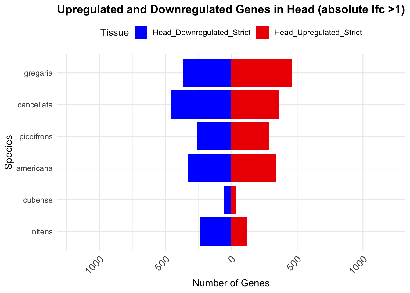
# Print the summary table for thorax
knitr::kable(summary_table_thorax, format = "markdown", caption = "Summary of differentially expressed genes in thorax per species")| Species | Thorax_Upregulated | Thorax_Downregulated | Thorax_Upregulated_Strict | Thorax_Downregulated_Strict |
|---|---|---|---|---|
| gregaria | 2194 | 2250 | 522 | 678 |
| piceifrons | 1639 | 1366 | 628 | 311 |
| cancellata | 723 | 730 | 304 | 365 |
| americana | 460 | 779 | 173 | 398 |
| cubense | 120 | 249 | 74 | 180 |
| nitens | 0 | 0 | 0 | 0 |
# Convert the summary table to a long format for thorax
summary_long_thorax <- summary_table_thorax %>%
  pivot_longer(cols = c(Thorax_Upregulated_Strict, Thorax_Downregulated_Strict),
               names_to = "Tissue", values_to = "Count")

# Adjust the values for downregulated genes to be negative
summary_long_thorax <- summary_long_thorax %>%
  mutate(Count = ifelse(Tissue == "Thorax_Downregulated_Strict", -Count, Count))

summary_long_thorax$Species <- factor(summary_long_thorax$Species, levels = species_order)

# Plot barplot for thorax
ggplot(summary_long_thorax, aes(x = Species, y = Count, fill = Tissue)) +
  geom_bar(stat = "identity", position = "stack") +
  labs(title = "Upregulated and Downregulated Genes in Thorax (absolute lfc >1)",
       x = "Species", y = "Number of Genes") +
  scale_fill_manual(values = c("Thorax_Upregulated_Strict" = "red2", "Thorax_Downregulated_Strict" = "blue")) +
  scale_y_continuous(labels = function(x) ifelse(x < 0, -x, x), limits = c(-1200, 1200)) +
  theme_minimal(base_size = 12) +
  theme(legend.position = "top",
        plot.title = element_text(hjust = 0.5, size = 14, face = "bold"),
        axis.text.x = element_text(size = 12, angle = 45, hjust = 1)) +
  coord_flip()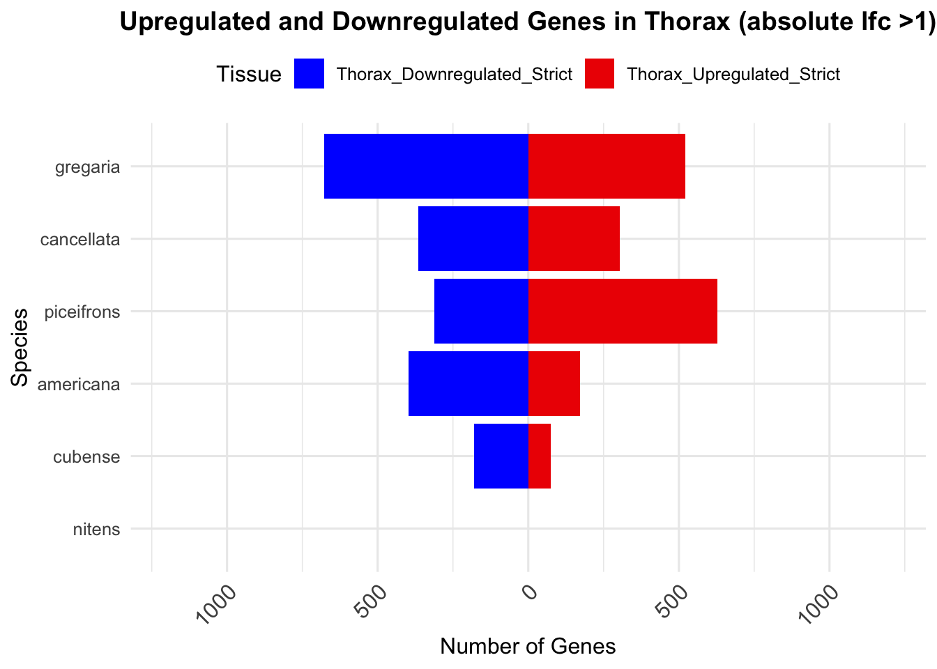
# Define custom colors for each GeneType
custom_colors <- c(
  "transcribed_pseudogene" = "#F4F1BB",  # Example color for transcribed_pseudogene
  "protein-coding" = "#9B57D3",         # Example color for protein-coding
  "lncRNA" = "#A5300F",                 # Example color for lncRNA
  "tRNA" = "#74D055FF",                   # Example color for tRNA
  "misc_RNA" = "#3B6978",               # Example color for misc_RNA
  "ncRNA" = "#29AF7FFF",                  # Example color for ncRNA
  "pseudogene" = "#81B29A",             # Example color for pseudogene
  "rRNA" = "#5982DB",                   # Example color for rRNA
  "snoRNA" = "#DCE318FF",                 # Example color for snoRNA
  "snRNA" = "#665EB8"                   # Example color for snRNA
)

# Use scale_fill_manual to map the custom colors to the GeneTypes
custom_color_scale <- scale_fill_manual(
  values = custom_colors
)
# Create an empty list to store the data for all species
all_species_data <- list()

# Loop through each species to process their data
for (species in species_list) {
  # Read the DESeq2 results for head and thorax
   head_results_file <- file.path(workDir, "DEG_results/Bulk_RNAseq/", paste0(species, "/Head/DESeq2_results_Head_", species ,".csv"))
    thorax_results_file <- file.path(workDir, "DEG_results/Bulk_RNAseq/", paste0(species, "/Thorax/DESeq2_results_Thorax_", species,".csv"))

  head_sigresults <- read.csv(head_results_file, stringsAsFactors = FALSE)
  thorax_sigresults <- read.csv(thorax_results_file, stringsAsFactors = FALSE)

  # Add GeneType and Species columns (from `allspecies_df`)
  head_results_merged <- merge(head_sigresults, allspecies_df[, c("GeneID", "GeneType", "Species")], by = "GeneID")
  thorax_results_merged <- merge(thorax_sigresults, allspecies_df[, c("GeneID", "GeneType", "Species")], by = "GeneID")

  # Count for upregulated and downregulated genes in head
  head_upregulated <- head_results_merged %>%
    filter(log2FoldChange > 1) %>%
    mutate(Regulation = "Upregulated", Tissue = "Head", Count = 1)

  head_downregulated <- head_results_merged %>%
    filter(log2FoldChange < -1) %>%
    mutate(Regulation = "Downregulated", Tissue = "Head", Count = -1)  # Mutate downregulated genes to negative

  # Combine upregulated and downregulated genes for head
  head_combined <- rbind(head_upregulated, head_downregulated)

  # Ensure all GeneTypes are represented for this species, even if they have no DEGs
  head_combined <- head_combined %>%
    complete(GeneType = unique(allspecies_df$GeneType),
             fill = list(Count = 0))  # Fill missing GeneTypes with Count = 0

  # Count for upregulated and downregulated genes in thorax
  thorax_upregulated <- thorax_results_merged %>%
    filter(log2FoldChange > 1) %>%
    mutate(Regulation = "Upregulated", Tissue = "Thorax", Count = 1)

  thorax_downregulated <- thorax_results_merged %>%
    filter(log2FoldChange < -1) %>%
    mutate(Regulation = "Downregulated", Tissue = "Thorax", Count = -1)  # Mutate downregulated genes to negative

  # Combine upregulated and downregulated genes for thorax
  thorax_combined <- rbind(thorax_upregulated, thorax_downregulated)

  # Ensure all GeneTypes are represented for this species in thorax, even if they have no DEGs
  thorax_combined <- thorax_combined %>%
    complete(GeneType = unique(allspecies_df$GeneType),
             fill = list(Count = 0))  # Fill missing GeneTypes with Count = 0

  # Combine data for head and thorax into one
  combined_data <- rbind(head_combined, thorax_combined)

  # Add species column to the data
  combined_data$Species <- species

  # Append the data to the list for all species
  all_species_data[[species]] <- combined_data
}

# Combine all species data into one data frame
final_data <- bind_rows(all_species_data)

# Reorder species according to the desired order
final_data$Species <- factor(final_data$Species, levels = species_order)

# Filter for head tissue only
final_data_head <- final_data %>% filter(Tissue == "Head")
final_data_thorax <- final_data %>% filter(Tissue == "Thorax")

# Create the barplot for all species and only head tissue
ggplot(final_data_head, aes(x = Species, y = Count, fill = GeneType)) +
  geom_bar(stat = "identity", position = "stack") +
  labs(title = "DEGs by Gene Biotype for Head (absolute lfc >1)",
       x = "Species",
       y = "Number of Genes") +
  custom_color_scale +
  scale_y_continuous(labels = function(x) ifelse(x < 0, -x, x), limits = c(-1200, 1200))+
theme_minimal(base_size = 12) +
  theme(legend.position = "top",
        plot.title = element_text(hjust = 0.5, size = 14, face = "bold"),
        axis.title.x = element_text(size = 14, face = "bold"),
        axis.title.y = element_text(size = 14, face = "bold"),
        axis.text.x = element_text(size = 12, angle = 45, hjust = 1),
        axis.text.y = element_text(size = 12),
        panel.grid.major.y = element_line(color = "grey90", linetype = "dashed"),
        panel.grid.minor = element_blank()) +
  coord_flip()  # Flip coordinates to make the plot horizontal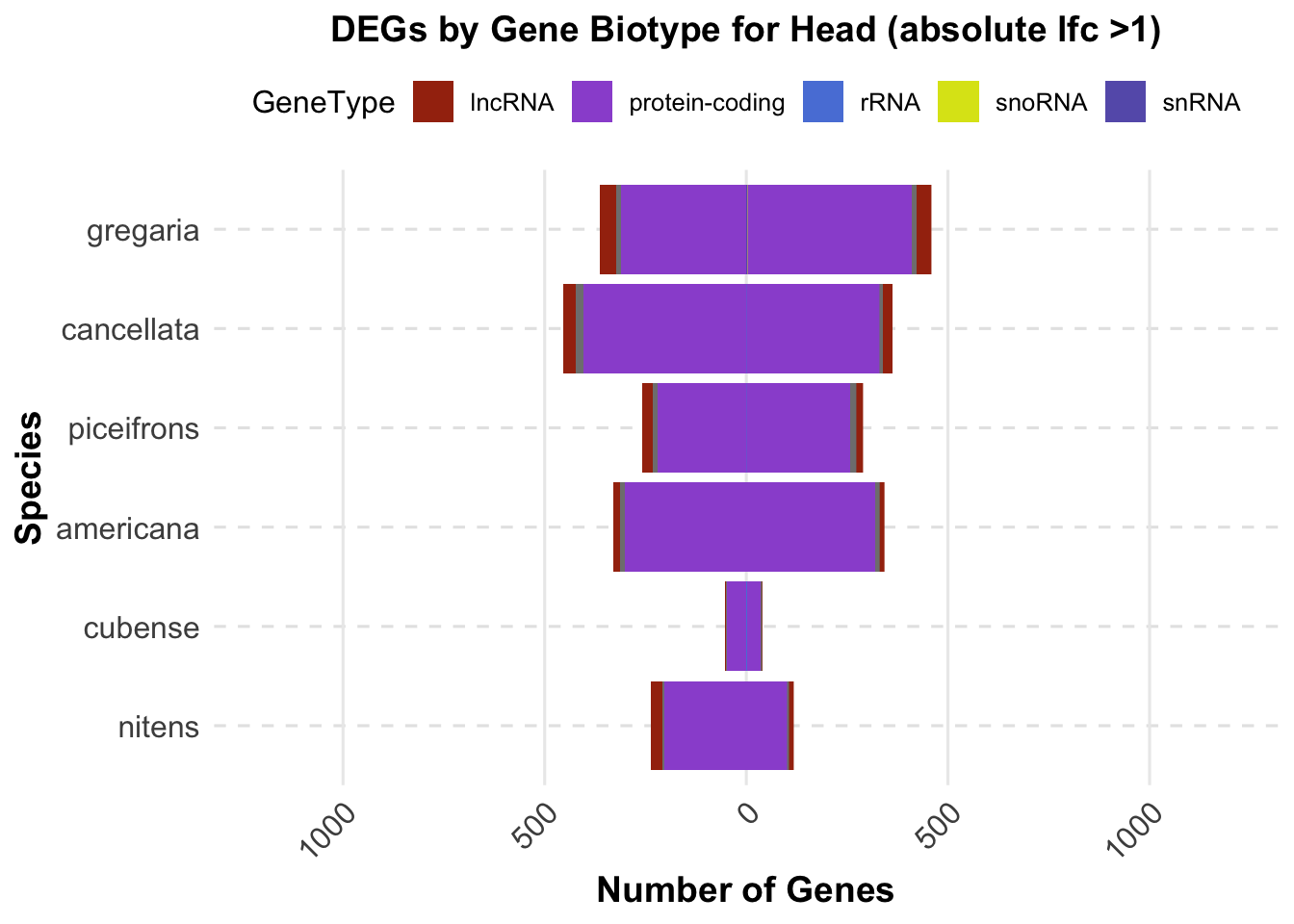
# Create the barplot for all species and only thorax tissue
ggplot(final_data_thorax, aes(x = Species, y = Count, fill = GeneType)) +
  geom_bar(stat = "identity", position = "stack") +
  labs(title = "DEGs by Gene Biotype for Thorax (absolute lfc >1)",
       x = "Species",
       y = "Number of Genes") +
  custom_color_scale +
  scale_y_continuous(labels = function(x) ifelse(x < 0, -x, x), limits = c(-1200, 1200))+
theme_minimal(base_size = 12) +
  theme(legend.position = "top",
        plot.title = element_text(hjust = 0.5, size = 14, face = "bold"),
        axis.title.x = element_text(size = 14, face = "bold"),
        axis.title.y = element_text(size = 14, face = "bold"),
        axis.text.x = element_text(size = 12, angle = 45, hjust = 1),
        axis.text.y = element_text(size = 12),
        panel.grid.major.y = element_line(color = "grey90", linetype = "dashed"),
        panel.grid.minor = element_blank()) +
  coord_flip()  # Flip coordinates to make the plot horizontal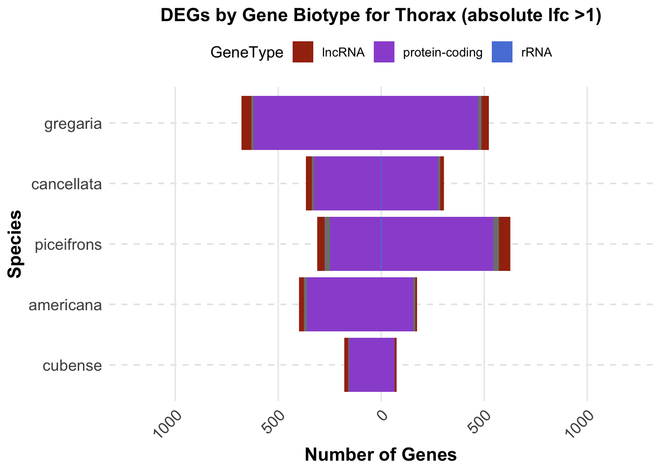
2. Overlap DEGs between tissues
gregaria
species <- "gregaria"  # Specify the species for which to generate plots

# Load DESeq2 results for head and thorax
head_file <- file.path(workDir, "DEG_results/Bulk_RNAseq/", paste0(species, "/Head/DESeq2_results_Head_", species,".csv"))
thorax_file <- file.path(workDir, "DEG_results/Bulk_RNAseq/", paste0(species, "/Thorax/DESeq2_results_Thorax_", species,".csv"))


head_data <- read.csv(head_file, stringsAsFactors = FALSE)
thorax_data <- read.csv(thorax_file, stringsAsFactors = FALSE)

# Check if data is empty and handle accordingly
if (nrow(head_data) == 0 || nrow(thorax_data) == 0) {
    message(paste("No data for species:", species))
} else {
    # Filter for significant DEGs and select upregulated and downregulated genes
    head_up <- head_data %>%
        filter(padj < 0.05 & log2FoldChange > 1) %>%
        select(GeneID = X)

    head_down <- head_data %>%
        filter(padj < 0.05 & log2FoldChange < -1) %>%
        select(GeneID = X)

    thorax_up <- thorax_data %>%
        filter(padj < 0.05 & log2FoldChange > 1) %>%
        select(GeneID = X)

    thorax_down <- thorax_data %>%
        filter(padj < 0.05 & log2FoldChange < -1) %>%
        select(GeneID = X)

    # Prepare data for Venn diagram
    venn_data <- list(
        Head_Upregulated = head_up$GeneID,
        Head_Downregulated = head_down$GeneID,
        Thorax_Upregulated = thorax_up$GeneID,
        Thorax_Downregulated = thorax_down$GeneID
    )

    # Generate the four-way Venn diagram with specified colors and legend outside
    venn_plot <- venn.diagram(
        x = venn_data,
        category.names = c("Head Upregulated", "Head Downregulated", "Thorax Upregulated", "Thorax Downregulated"),
        filename = NULL,
        output = TRUE,
        fill = c("red", "skyblue", "orange", "blue"),  # Set colors for upregulated and downregulated
        alpha = 0.5,
        cex = 2,  # Text size for numbers
        cat.cex = 0,  # Text size for category labels
        cat.pos = c(0, 0, 0, 0),  # Position to center labels
        cat.dist = c(0.1, 0.1, 0.1, 0.1),  # Distance between category labels and circles
        main = paste("Venn Diagram of DEGs for S.", species),
        main.cex = 1.2,  # Size of the main title
        cat.col = c("red", "skyblue", "orange", "blue")  # Color the category labels
    )

    # Clear the current plotting area before drawing the next Venn diagram
    grid.newpage()

    # Display the Venn diagram
    grid.draw(venn_plot)

    # Manually create a custom legend
    legend_labels <- c("Head Up", "Head Down", "Thorax Up", "Thorax Down")
    legend_colors <- c("red", "skyblue", "orange", "blue")

    # Positioning the legend lower on the right side of the plot
    legend_x <- unit(0.85, "npc")  # Adjust x position
    legend_y <- unit(0.2, "npc")    # Lower the legend vertically

    # Draw the legend
    for (i in 1:length(legend_labels)) {
        grid.rect(x = legend_x, y = legend_y - unit((i - 1) * 0.05, "npc"),
                  width = unit(0.02, "npc"), height = unit(0.02, "npc"),
                  gp = gpar(fill = legend_colors[i], col = NA))
        grid.text(label = legend_labels[i], x = legend_x + unit(0.05, "npc"),
                  y = legend_y - unit((i - 1) * 0.05, "npc"),
                  just = "left", gp = gpar(cex = 0.8))
    }

    # Scatter plot for overlapping genes
    # Filter significant DEGs for both head and thorax
    head_sig_genes <- head_data %>%
        filter(padj < 0.05 & abs(log2FoldChange) > 1) %>%
        select(GeneID = X, log2FoldChange, padj)

    thorax_sig_genes <- thorax_data %>%
        filter(padj < 0.05 & abs(log2FoldChange) > 1) %>%
        select(GeneID = X, log2FoldChange, padj)

    # Find overlapping genes based on GeneID
    overlapping_genes <- inner_join(head_sig_genes, thorax_sig_genes, by = "GeneID", suffix = c("_head", "_thorax"))

    # Save the overlapping genes to a CSV file
    output_file <- file.path(workDir, "overlap/Bulk_RNAseq", paste0("overlapping_genes_head_thorax_", species, ".csv"))
    write.csv(overlapping_genes, output_file, row.names = FALSE)

    # Plot overlapping genes with scatter plot
    p <- ggplot(overlapping_genes, aes(x = log2FoldChange_head, y = log2FoldChange_thorax)) +
        geom_point(aes(color = case_when(
            log2FoldChange_head > 0 & log2FoldChange_thorax > 0 ~ "Upregulated in Both",
            log2FoldChange_head < 0 & log2FoldChange_thorax < 0 ~ "Downregulated in Both",
            log2FoldChange_head > 0 & log2FoldChange_thorax < 0 ~ "Up in Head, Down in Thorax",
            log2FoldChange_head < 0 & log2FoldChange_thorax > 0 ~ "Down in Head, Up in Thorax"
        )), size = 3, alpha = 0.7) +
        geom_abline(slope = 1, intercept = 0, linetype = "dashed", color = "gray") +
        labs(
            x = "Log2 Fold Change (Head)",
            y = "Log2 Fold Change (Thorax)",
            color = "Regulation Pattern",
            title = "Comparison of Log2 Fold Changes in Overlapping Genes",
            subtitle = paste("Head vs. Thorax in", species)
        ) +
        theme_minimal() +
        theme(
            plot.title = element_text(size = 16, face = "bold"),
            plot.subtitle = element_text(size = 12, face = "italic"),
            legend.position = "top"
        ) +
        scale_color_manual(values = c(
            "Upregulated in Both" = "red",
            "Downregulated in Both" = "blue",
            "Up in Head, Down in Thorax" = "purple",
            "Down in Head, Up in Thorax" = "green"
        ))

    # Save the scatter plot
    ggsave(filename = file.path(workDir, "overlap/Bulk_RNAseq", paste0("scatter_plot_overlapping_genes_", species, ".png")), plot = p)

    # Display the scatter plot
    print(p)
}
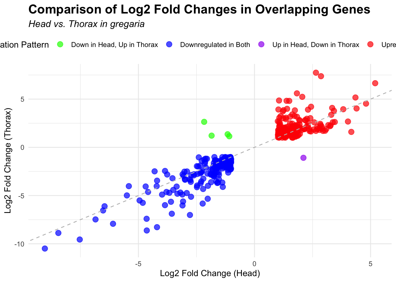
piceifrons
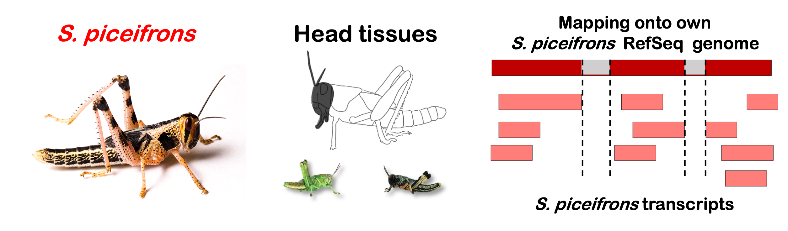
species <- "piceifrons"  # Specify the species for which to generate plots

# Load DESeq2 results for head and thorax
head_file <- file.path(workDir, "DEG_results/Bulk_RNAseq/", paste0(species, "/Head/DESeq2_results_Head_", species,".csv"))
thorax_file <- file.path(workDir, "DEG_results/Bulk_RNAseq/", paste0(species, "/Thorax/DESeq2_results_Thorax_", species,".csv"))

head_data <- read.csv(head_file, stringsAsFactors = FALSE)
thorax_data <- read.csv(thorax_file, stringsAsFactors = FALSE)

# Check if data is empty and handle accordingly
if (nrow(head_data) == 0 || nrow(thorax_data) == 0) {
    message(paste("No data for species:", species))
} else {
    # Filter for significant DEGs and select upregulated and downregulated genes
    head_up <- head_data %>%
        filter(padj < 0.05 & log2FoldChange > 1) %>%
        select(GeneID = X)

    head_down <- head_data %>%
        filter(padj < 0.05 & log2FoldChange < -1) %>%
        select(GeneID = X)

    thorax_up <- thorax_data %>%
        filter(padj < 0.05 & log2FoldChange > 1) %>%
        select(GeneID = X)

    thorax_down <- thorax_data %>%
        filter(padj < 0.05 & log2FoldChange < -1) %>%
        select(GeneID = X)

    # Prepare data for Venn diagram
    venn_data <- list(
        Head_Upregulated = head_up$GeneID,
        Head_Downregulated = head_down$GeneID,
        Thorax_Upregulated = thorax_up$GeneID,
        Thorax_Downregulated = thorax_down$GeneID
    )

    # Generate the four-way Venn diagram with specified colors and legend outside
    venn_plot <- venn.diagram(
        x = venn_data,
        category.names = c("Head Upregulated", "Head Downregulated", "Thorax Upregulated", "Thorax Downregulated"),
        filename = NULL,
        output = TRUE,
        fill = c("red", "skyblue", "orange", "blue"),  # Set colors for upregulated and downregulated
        alpha = 0.5,
        cex = 2,  # Text size for numbers
        cat.cex = 0,  # Text size for category labels
        cat.pos = c(0, 0, 0, 0),  # Position to center labels
        cat.dist = c(0.1, 0.1, 0.1, 0.1),  # Distance between category labels and circles
        main = paste("Venn Diagram of DEGs for S.", species),
        main.cex = 1.2,  # Size of the main title
        cat.col = c("red", "skyblue", "orange", "blue")  # Color the category labels
    )

    # Clear the current plotting area before drawing the next Venn diagram
    grid.newpage()

    # Display the Venn diagram
    grid.draw(venn_plot)

    # Manually create a custom legend
    legend_labels <- c("Head Up", "Head Down", "Thorax Up", "Thorax Down")
    legend_colors <- c("red", "skyblue", "orange", "blue")

    # Positioning the legend lower on the right side of the plot
    legend_x <- unit(0.85, "npc")  # Adjust x position
    legend_y <- unit(0.2, "npc")    # Lower the legend vertically

    # Draw the legend
    for (i in 1:length(legend_labels)) {
        grid.rect(x = legend_x, y = legend_y - unit((i - 1) * 0.05, "npc"),
                  width = unit(0.02, "npc"), height = unit(0.02, "npc"),
                  gp = gpar(fill = legend_colors[i], col = NA))
        grid.text(label = legend_labels[i], x = legend_x + unit(0.05, "npc"),
                  y = legend_y - unit((i - 1) * 0.05, "npc"),
                  just = "left", gp = gpar(cex = 0.8))
    }

    # Scatter plot for overlapping genes
    # Filter significant DEGs for both head and thorax
    head_sig_genes <- head_data %>%
        filter(padj < 0.05 & abs(log2FoldChange) > 1) %>%
        select(GeneID = X, log2FoldChange, padj)

    thorax_sig_genes <- thorax_data %>%
        filter(padj < 0.05 & abs(log2FoldChange) > 1) %>%
        select(GeneID = X, log2FoldChange, padj)

    # Find overlapping genes based on GeneID
    overlapping_genes <- inner_join(head_sig_genes, thorax_sig_genes, by = "GeneID", suffix = c("_head", "_thorax"))

    # Save the overlapping genes to a CSV file
    output_file <- file.path(workDir, "overlap/Bulk_RNAseq", paste0("overlapping_genes_head_thorax_", species, ".csv"))
    write.csv(overlapping_genes, output_file, row.names = FALSE)

    # Plot overlapping genes with scatter plot
    p <- ggplot(overlapping_genes, aes(x = log2FoldChange_head, y = log2FoldChange_thorax)) +
        geom_point(aes(color = case_when(
            log2FoldChange_head > 0 & log2FoldChange_thorax > 0 ~ "Upregulated in Both",
            log2FoldChange_head < 0 & log2FoldChange_thorax < 0 ~ "Downregulated in Both",
            log2FoldChange_head > 0 & log2FoldChange_thorax < 0 ~ "Up in Head, Down in Thorax",
            log2FoldChange_head < 0 & log2FoldChange_thorax > 0 ~ "Down in Head, Up in Thorax"
        )), size = 3, alpha = 0.7) +
        geom_abline(slope = 1, intercept = 0, linetype = "dashed", color = "gray") +
        labs(
            x = "Log2 Fold Change (Head)",
            y = "Log2 Fold Change (Thorax)",
            color = "Regulation Pattern",
            title = "Comparison of Log2 Fold Changes in Overlapping Genes",
            subtitle = paste("Head vs. Thorax in", species)
        ) +
        theme_minimal() +
        theme(
            plot.title = element_text(size = 16, face = "bold"),
            plot.subtitle = element_text(size = 12, face = "italic"),
            legend.position = "top"
        ) +
        scale_color_manual(values = c(
            "Upregulated in Both" = "red",
            "Downregulated in Both" = "blue",
            "Up in Head, Down in Thorax" = "purple",
            "Down in Head, Up in Thorax" = "green"
        ))

    # Save the scatter plot
    ggsave(filename = file.path(workDir, "overlap/Bulk_RNAseq", paste0("scatter_plot_overlapping_genes_", species, ".png")), plot = p)

    # Display the scatter plot
    print(p)
}
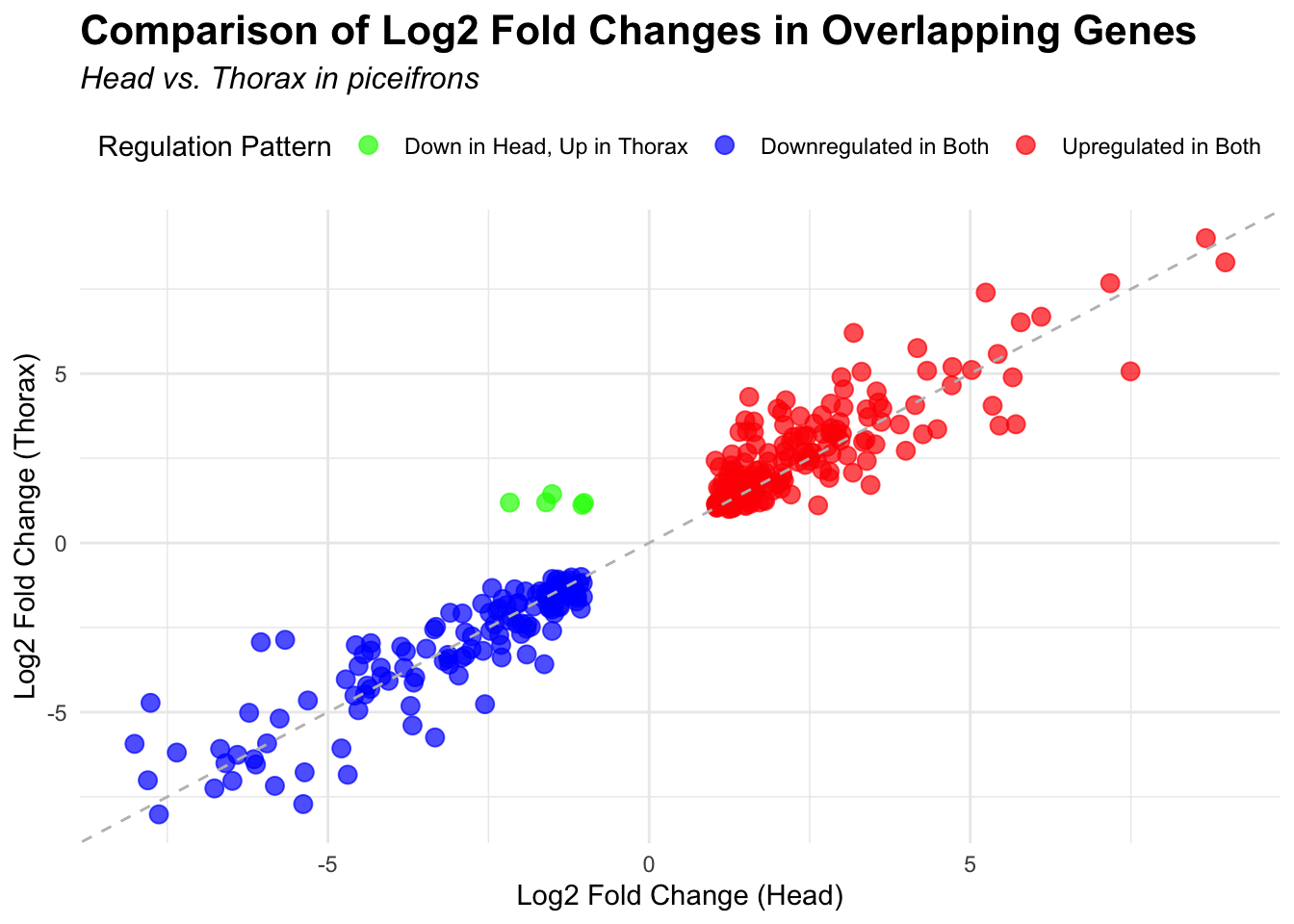
cancellata
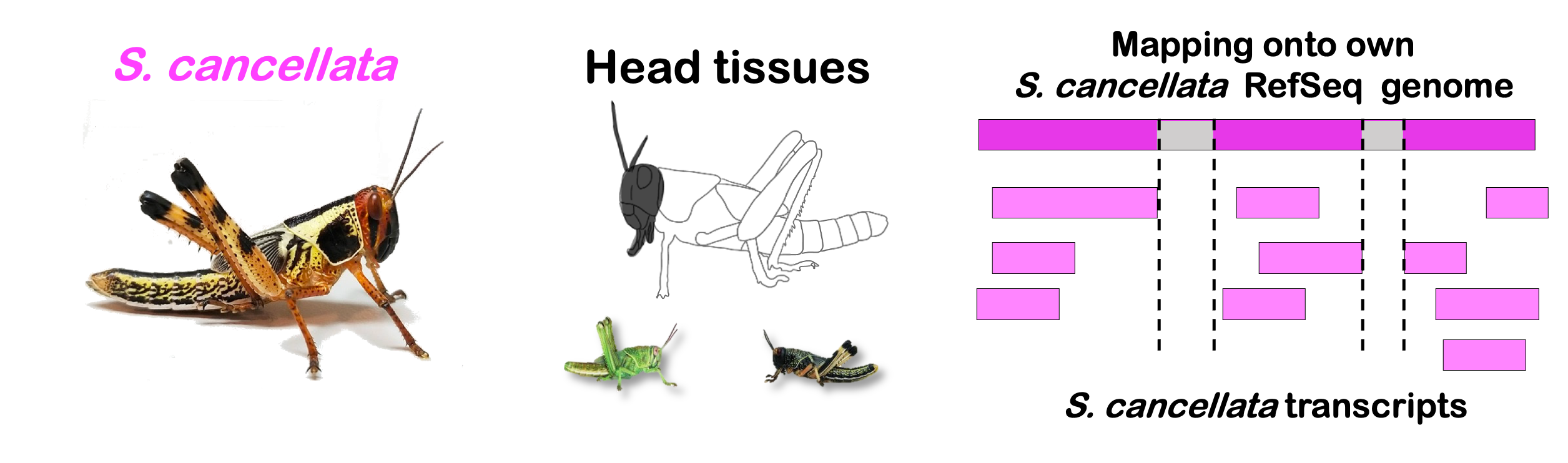
species <- "cancellata"  # Specify the species for which to generate plots

# Load DESeq2 results for head and thorax
head_file <- file.path(workDir, "DEG_results/Bulk_RNAseq/", paste0(species, "/Head/DESeq2_results_Head_", species,".csv"))
thorax_file <- file.path(workDir, "DEG_results/Bulk_RNAseq/", paste0(species, "/Thorax/DESeq2_results_Thorax_", species,".csv"))

head_data <- read.csv(head_file, stringsAsFactors = FALSE)
thorax_data <- read.csv(thorax_file, stringsAsFactors = FALSE)

# Check if data is empty and handle accordingly
if (nrow(head_data) == 0 || nrow(thorax_data) == 0) {
    message(paste("No data for species:", species))
} else {
    # Filter for significant DEGs and select upregulated and downregulated genes
    head_up <- head_data %>%
        filter(padj < 0.05 & log2FoldChange > 1) %>%
        select(GeneID = X)

    head_down <- head_data %>%
        filter(padj < 0.05 & log2FoldChange < -1) %>%
        select(GeneID = X)

    thorax_up <- thorax_data %>%
        filter(padj < 0.05 & log2FoldChange > 1) %>%
        select(GeneID = X)

    thorax_down <- thorax_data %>%
        filter(padj < 0.05 & log2FoldChange < -1) %>%
        select(GeneID = X)

    # Prepare data for Venn diagram
    venn_data <- list(
        Head_Upregulated = head_up$GeneID,
        Head_Downregulated = head_down$GeneID,
        Thorax_Upregulated = thorax_up$GeneID,
        Thorax_Downregulated = thorax_down$GeneID
    )

    # Generate the four-way Venn diagram with specified colors and legend outside
    venn_plot <- venn.diagram(
        x = venn_data,
        category.names = c("Head Upregulated", "Head Downregulated", "Thorax Upregulated", "Thorax Downregulated"),
        filename = NULL,
        output = TRUE,
        fill = c("red", "skyblue", "orange", "blue"),  # Set colors for upregulated and downregulated
        alpha = 0.5,
        cex = 2,  # Text size for numbers
        cat.cex = 0,  # Text size for category labels
        cat.pos = c(0, 0, 0, 0),  # Position to center labels
        cat.dist = c(0.1, 0.1, 0.1, 0.1),  # Distance between category labels and circles
        main = paste("Venn Diagram of DEGs for S.", species),
        main.cex = 1.2,  # Size of the main title
        cat.col = c("red", "skyblue", "orange", "blue")  # Color the category labels
    )

    # Clear the current plotting area before drawing the next Venn diagram
    grid.newpage()

    # Display the Venn diagram
    grid.draw(venn_plot)

    # Manually create a custom legend
    legend_labels <- c("Head Up", "Head Down", "Thorax Up", "Thorax Down")
    legend_colors <- c("red", "skyblue", "orange", "blue")

    # Positioning the legend lower on the right side of the plot
    legend_x <- unit(0.85, "npc")  # Adjust x position
    legend_y <- unit(0.2, "npc")    # Lower the legend vertically

    # Draw the legend
    for (i in 1:length(legend_labels)) {
        grid.rect(x = legend_x, y = legend_y - unit((i - 1) * 0.05, "npc"),
                  width = unit(0.02, "npc"), height = unit(0.02, "npc"),
                  gp = gpar(fill = legend_colors[i], col = NA))
        grid.text(label = legend_labels[i], x = legend_x + unit(0.05, "npc"),
                  y = legend_y - unit((i - 1) * 0.05, "npc"),
                  just = "left", gp = gpar(cex = 0.8))
    }

    # Scatter plot for overlapping genes
    # Filter significant DEGs for both head and thorax
    head_sig_genes <- head_data %>%
        filter(padj < 0.05 & abs(log2FoldChange) > 1) %>%
        select(GeneID = X, log2FoldChange, padj)

    thorax_sig_genes <- thorax_data %>%
        filter(padj < 0.05 & abs(log2FoldChange) > 1) %>%
        select(GeneID = X, log2FoldChange, padj)

    # Find overlapping genes based on GeneID
    overlapping_genes <- inner_join(head_sig_genes, thorax_sig_genes, by = "GeneID", suffix = c("_head", "_thorax"))

    # Save the overlapping genes to a CSV file
    output_file <- file.path(workDir, "overlap/Bulk_RNAseq", paste0("overlapping_genes_head_thorax_", species, ".csv"))
    write.csv(overlapping_genes, output_file, row.names = FALSE)

    # Plot overlapping genes with scatter plot
    p <- ggplot(overlapping_genes, aes(x = log2FoldChange_head, y = log2FoldChange_thorax)) +
        geom_point(aes(color = case_when(
            log2FoldChange_head > 0 & log2FoldChange_thorax > 0 ~ "Upregulated in Both",
            log2FoldChange_head < 0 & log2FoldChange_thorax < 0 ~ "Downregulated in Both",
            log2FoldChange_head > 0 & log2FoldChange_thorax < 0 ~ "Up in Head, Down in Thorax",
            log2FoldChange_head < 0 & log2FoldChange_thorax > 0 ~ "Down in Head, Up in Thorax"
        )), size = 3, alpha = 0.7) +
        geom_abline(slope = 1, intercept = 0, linetype = "dashed", color = "gray") +
        labs(
            x = "Log2 Fold Change (Head)",
            y = "Log2 Fold Change (Thorax)",
            color = "Regulation Pattern",
            title = "Comparison of Log2 Fold Changes in Overlapping Genes",
            subtitle = paste("Head vs. Thorax in", species)
        ) +
        theme_minimal() +
        theme(
            plot.title = element_text(size = 16, face = "bold"),
            plot.subtitle = element_text(size = 12, face = "italic"),
            legend.position = "top"
        ) +
        scale_color_manual(values = c(
            "Upregulated in Both" = "red",
            "Downregulated in Both" = "blue",
            "Up in Head, Down in Thorax" = "purple",
            "Down in Head, Up in Thorax" = "green"
        ))

    # Save the scatter plot
    ggsave(filename = file.path(workDir, "overlap/Bulk_RNAseq", paste0("scatter_plot_overlapping_genes_", species, ".png")), plot = p)

    # Display the scatter plot
    print(p)
}
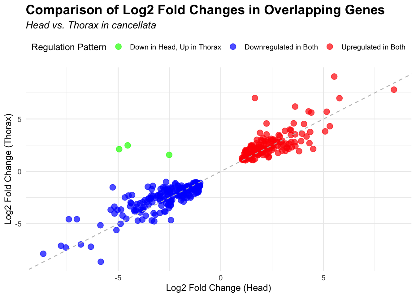
americana
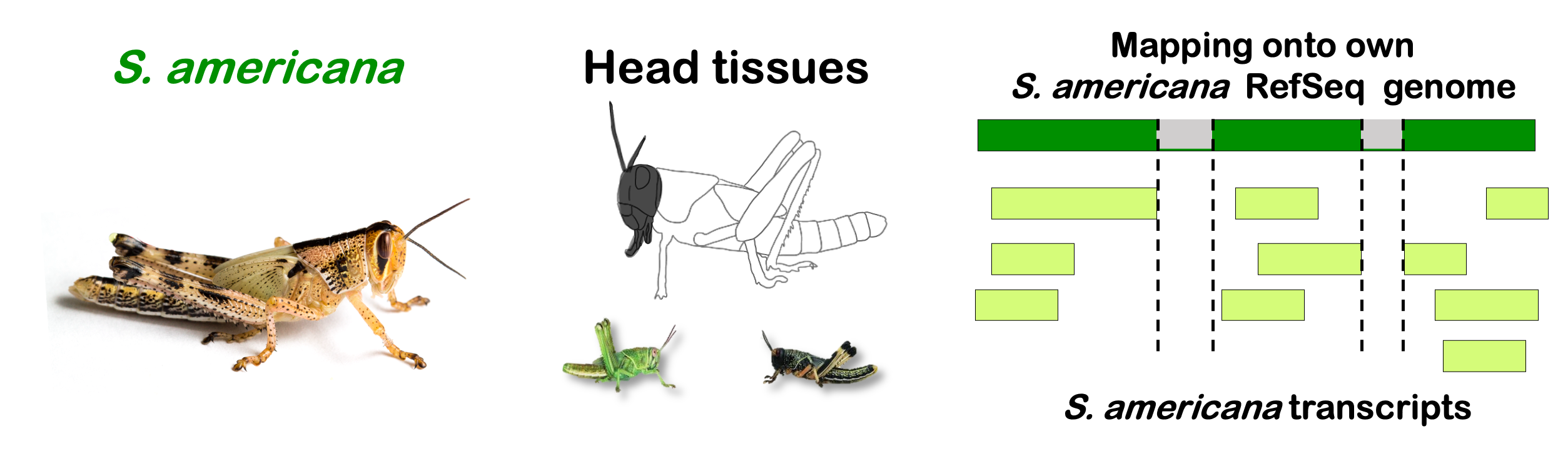
species <- "americana"  # Specify the species for which to generate plots

# Load DESeq2 results for head and thorax
head_file <- file.path(workDir, "DEG_results/Bulk_RNAseq/", paste0(species, "/Head/DESeq2_results_Head_", species,".csv"))
thorax_file <- file.path(workDir, "DEG_results/Bulk_RNAseq/", paste0(species, "/Thorax/DESeq2_results_Thorax_", species,".csv"))

head_data <- read.csv(head_file, stringsAsFactors = FALSE)
thorax_data <- read.csv(thorax_file, stringsAsFactors = FALSE)

# Check if data is empty and handle accordingly
if (nrow(head_data) == 0 || nrow(thorax_data) == 0) {
    message(paste("No data for species:", species))
} else {
    # Filter for significant DEGs and select upregulated and downregulated genes
    head_up <- head_data %>%
        filter(padj < 0.05 & log2FoldChange > 1) %>%
        select(GeneID = X)

    head_down <- head_data %>%
        filter(padj < 0.05 & log2FoldChange < -1) %>%
        select(GeneID = X)

    thorax_up <- thorax_data %>%
        filter(padj < 0.05 & log2FoldChange > 1) %>%
        select(GeneID = X)

    thorax_down <- thorax_data %>%
        filter(padj < 0.05 & log2FoldChange < -1) %>%
        select(GeneID = X)

    # Prepare data for Venn diagram
    venn_data <- list(
        Head_Upregulated = head_up$GeneID,
        Head_Downregulated = head_down$GeneID,
        Thorax_Upregulated = thorax_up$GeneID,
        Thorax_Downregulated = thorax_down$GeneID
    )

    # Generate the four-way Venn diagram with specified colors and legend outside
    venn_plot <- venn.diagram(
        x = venn_data,
        category.names = c("Head Upregulated", "Head Downregulated", "Thorax Upregulated", "Thorax Downregulated"),
        filename = NULL,
        output = TRUE,
        fill = c("red", "skyblue", "orange", "blue"),  # Set colors for upregulated and downregulated
        alpha = 0.5,
        cex = 2,  # Text size for numbers
        cat.cex = 0,  # Text size for category labels
        cat.pos = c(0, 0, 0, 0),  # Position to center labels
        cat.dist = c(0.1, 0.1, 0.1, 0.1),  # Distance between category labels and circles
        main = paste("Venn Diagram of DEGs for S.", species),
        main.cex = 1.2,  # Size of the main title
        cat.col = c("red", "skyblue", "orange", "blue")  # Color the category labels
    )

    # Clear the current plotting area before drawing the next Venn diagram
    grid.newpage()

    # Display the Venn diagram
    grid.draw(venn_plot)

    # Manually create a custom legend
    legend_labels <- c("Head Up", "Head Down", "Thorax Up", "Thorax Down")
    legend_colors <- c("red", "skyblue", "orange", "blue")

    # Positioning the legend lower on the right side of the plot
    legend_x <- unit(0.85, "npc")  # Adjust x position
    legend_y <- unit(0.2, "npc")    # Lower the legend vertically

    # Draw the legend
    for (i in 1:length(legend_labels)) {
        grid.rect(x = legend_x, y = legend_y - unit((i - 1) * 0.05, "npc"),
                  width = unit(0.02, "npc"), height = unit(0.02, "npc"),
                  gp = gpar(fill = legend_colors[i], col = NA))
        grid.text(label = legend_labels[i], x = legend_x + unit(0.05, "npc"),
                  y = legend_y - unit((i - 1) * 0.05, "npc"),
                  just = "left", gp = gpar(cex = 0.8))
    }

    # Scatter plot for overlapping genes
    # Filter significant DEGs for both head and thorax
    head_sig_genes <- head_data %>%
        filter(padj < 0.05 & abs(log2FoldChange) > 1) %>%
        select(GeneID = X, log2FoldChange, padj)

    thorax_sig_genes <- thorax_data %>%
        filter(padj < 0.05 & abs(log2FoldChange) > 1) %>%
        select(GeneID = X, log2FoldChange, padj)

    # Find overlapping genes based on GeneID
    overlapping_genes <- inner_join(head_sig_genes, thorax_sig_genes, by = "GeneID", suffix = c("_head", "_thorax"))

    # Save the overlapping genes to a CSV file
    output_file <- file.path(workDir, "overlap/Bulk_RNAseq", paste0("overlapping_genes_head_thorax_", species, ".csv"))
    write.csv(overlapping_genes, output_file, row.names = FALSE)

    # Plot overlapping genes with scatter plot
    p <- ggplot(overlapping_genes, aes(x = log2FoldChange_head, y = log2FoldChange_thorax)) +
        geom_point(aes(color = case_when(
            log2FoldChange_head > 0 & log2FoldChange_thorax > 0 ~ "Upregulated in Both",
            log2FoldChange_head < 0 & log2FoldChange_thorax < 0 ~ "Downregulated in Both",
            log2FoldChange_head > 0 & log2FoldChange_thorax < 0 ~ "Up in Head, Down in Thorax",
            log2FoldChange_head < 0 & log2FoldChange_thorax > 0 ~ "Down in Head, Up in Thorax"
        )), size = 3, alpha = 0.7) +
        geom_abline(slope = 1, intercept = 0, linetype = "dashed", color = "gray") +
        labs(
            x = "Log2 Fold Change (Head)",
            y = "Log2 Fold Change (Thorax)",
            color = "Regulation Pattern",
            title = "Comparison of Log2 Fold Changes in Overlapping Genes",
            subtitle = paste("Head vs. Thorax in", species)
        ) +
        theme_minimal() +
        theme(
            plot.title = element_text(size = 16, face = "bold"),
            plot.subtitle = element_text(size = 12, face = "italic"),
            legend.position = "top"
        ) +
        scale_color_manual(values = c(
            "Upregulated in Both" = "red",
            "Downregulated in Both" = "blue",
            "Up in Head, Down in Thorax" = "purple",
            "Down in Head, Up in Thorax" = "green"
        ))

    # Save the scatter plot
    ggsave(filename = file.path(workDir, "overlap/Bulk_RNAseq", paste0("scatter_plot_overlapping_genes_", species, ".png")), plot = p)

    # Display the scatter plot
    print(p)
}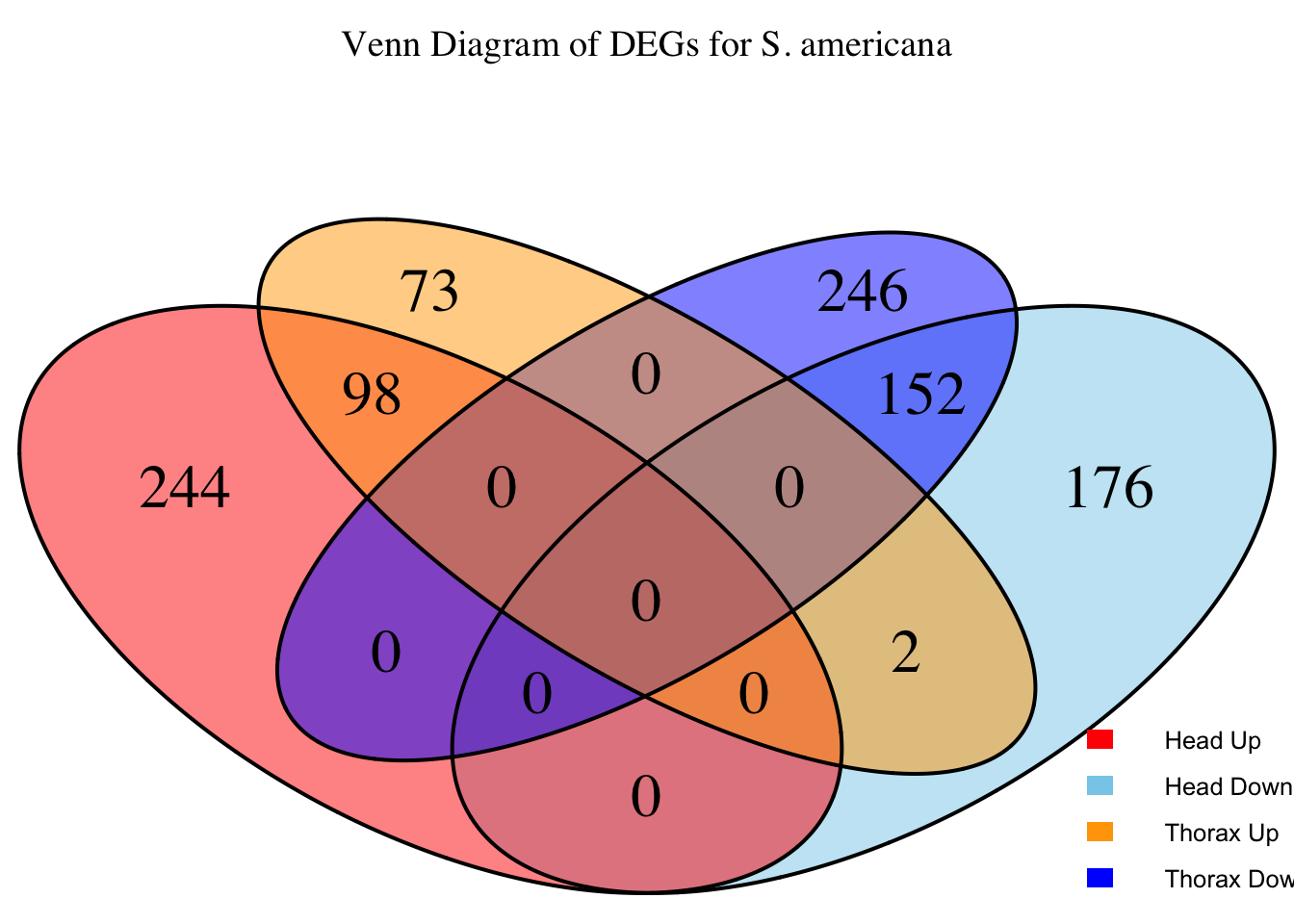
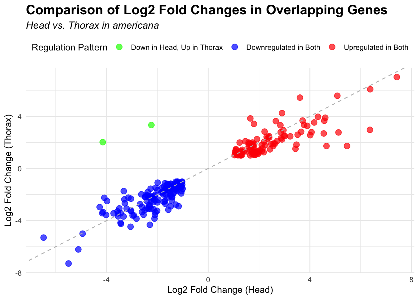
cubense
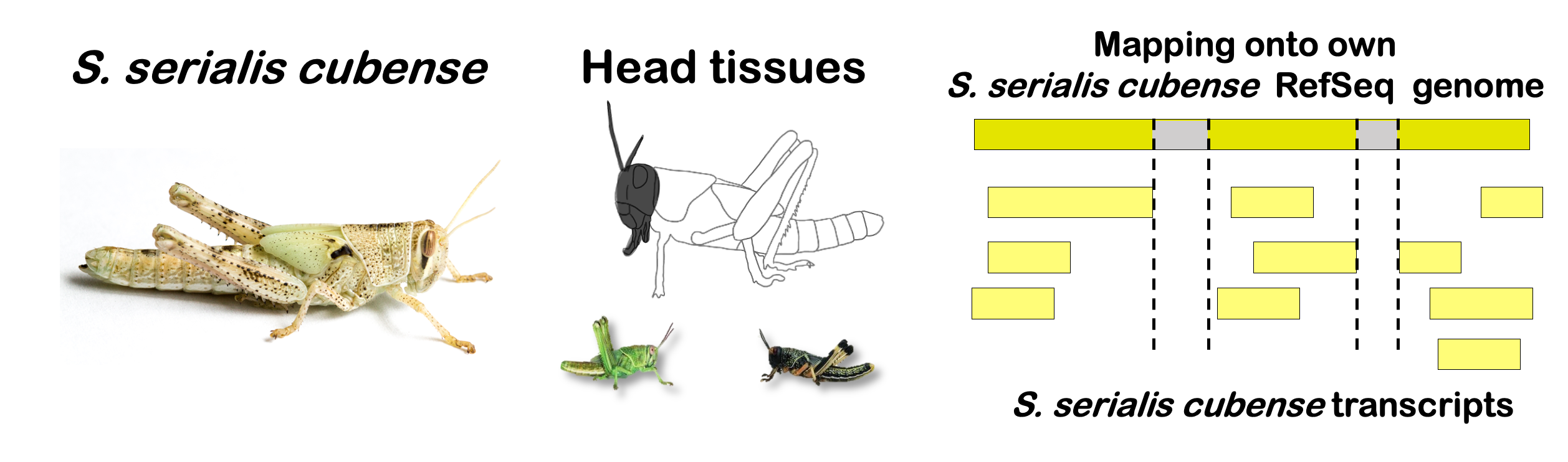
species <- "cubense"  # Specify the species for which to generate plots

# Load DESeq2 results for head and thorax
head_file <- file.path(workDir, "DEG_results/Bulk_RNAseq/", paste0(species, "/Head/DESeq2_results_Head_", species,".csv"))
thorax_file <- file.path(workDir, "DEG_results/Bulk_RNAseq/", paste0(species, "/Thorax/DESeq2_results_Thorax_", species,".csv"))

head_data <- read.csv(head_file, stringsAsFactors = FALSE)
thorax_data <- read.csv(thorax_file, stringsAsFactors = FALSE)

# Check if data is empty and handle accordingly
if (nrow(head_data) == 0 || nrow(thorax_data) == 0) {
    message(paste("No data for species:", species))
} else {
    # Filter for significant DEGs and select upregulated and downregulated genes
    head_up <- head_data %>%
        filter(padj < 0.05 & log2FoldChange > 1) %>%
        select(GeneID = X)

    head_down <- head_data %>%
        filter(padj < 0.05 & log2FoldChange < -1) %>%
        select(GeneID = X)

    thorax_up <- thorax_data %>%
        filter(padj < 0.05 & log2FoldChange > 1) %>%
        select(GeneID = X)

    thorax_down <- thorax_data %>%
        filter(padj < 0.05 & log2FoldChange < -1) %>%
        select(GeneID = X)

    # Prepare data for Venn diagram
    venn_data <- list(
        Head_Upregulated = head_up$GeneID,
        Head_Downregulated = head_down$GeneID,
        Thorax_Upregulated = thorax_up$GeneID,
        Thorax_Downregulated = thorax_down$GeneID
    )

    # Generate the four-way Venn diagram with specified colors and legend outside
    venn_plot <- venn.diagram(
        x = venn_data,
        category.names = c("Head Upregulated", "Head Downregulated", "Thorax Upregulated", "Thorax Downregulated"),
        filename = NULL,
        output = TRUE,
        fill = c("red", "skyblue", "orange", "blue"),  # Set colors for upregulated and downregulated
        alpha = 0.5,
        cex = 2,  # Text size for numbers
        cat.cex = 0,  # Text size for category labels
        cat.pos = c(0, 0, 0, 0),  # Position to center labels
        cat.dist = c(0.1, 0.1, 0.1, 0.1),  # Distance between category labels and circles
        main = paste("Venn Diagram of DEGs for S.", species),
        main.cex = 1.2,  # Size of the main title
        cat.col = c("red", "skyblue", "orange", "blue")  # Color the category labels
    )

    # Clear the current plotting area before drawing the next Venn diagram
    grid.newpage()

    # Display the Venn diagram
    grid.draw(venn_plot)

    # Manually create a custom legend
    legend_labels <- c("Head Up", "Head Down", "Thorax Up", "Thorax Down")
    legend_colors <- c("red", "skyblue", "orange", "blue")

    # Positioning the legend lower on the right side of the plot
    legend_x <- unit(0.85, "npc")  # Adjust x position
    legend_y <- unit(0.2, "npc")    # Lower the legend vertically

    # Draw the legend
    for (i in 1:length(legend_labels)) {
        grid.rect(x = legend_x, y = legend_y - unit((i - 1) * 0.05, "npc"),
                  width = unit(0.02, "npc"), height = unit(0.02, "npc"),
                  gp = gpar(fill = legend_colors[i], col = NA))
        grid.text(label = legend_labels[i], x = legend_x + unit(0.05, "npc"),
                  y = legend_y - unit((i - 1) * 0.05, "npc"),
                  just = "left", gp = gpar(cex = 0.8))
    }

    # Scatter plot for overlapping genes
    # Filter significant DEGs for both head and thorax
    head_sig_genes <- head_data %>%
        filter(padj < 0.05 & abs(log2FoldChange) > 1) %>%
        select(GeneID = X, log2FoldChange, padj)

    thorax_sig_genes <- thorax_data %>%
        filter(padj < 0.05 & abs(log2FoldChange) > 1) %>%
        select(GeneID = X, log2FoldChange, padj)

    # Find overlapping genes based on GeneID
    overlapping_genes <- inner_join(head_sig_genes, thorax_sig_genes, by = "GeneID", suffix = c("_head", "_thorax"))

    # Save the overlapping genes to a CSV file
    output_file <- file.path(workDir, "overlap/Bulk_RNAseq", paste0("overlapping_genes_head_thorax_", species, ".csv"))
    write.csv(overlapping_genes, output_file, row.names = FALSE)

    # Plot overlapping genes with scatter plot
    p <- ggplot(overlapping_genes, aes(x = log2FoldChange_head, y = log2FoldChange_thorax)) +
        geom_point(aes(color = case_when(
            log2FoldChange_head > 0 & log2FoldChange_thorax > 0 ~ "Upregulated in Both",
            log2FoldChange_head < 0 & log2FoldChange_thorax < 0 ~ "Downregulated in Both",
            log2FoldChange_head > 0 & log2FoldChange_thorax < 0 ~ "Up in Head, Down in Thorax",
            log2FoldChange_head < 0 & log2FoldChange_thorax > 0 ~ "Down in Head, Up in Thorax"
        )), size = 3, alpha = 0.7) +
        geom_abline(slope = 1, intercept = 0, linetype = "dashed", color = "gray") +
        labs(
            x = "Log2 Fold Change (Head)",
            y = "Log2 Fold Change (Thorax)",
            color = "Regulation Pattern",
            title = "Comparison of Log2 Fold Changes in Overlapping Genes",
            subtitle = paste("Head vs. Thorax in", species)
        ) +
        theme_minimal() +
        theme(
            plot.title = element_text(size = 16, face = "bold"),
            plot.subtitle = element_text(size = 12, face = "italic"),
            legend.position = "top"
        ) +
        scale_color_manual(values = c(
            "Upregulated in Both" = "red",
            "Downregulated in Both" = "blue",
            "Up in Head, Down in Thorax" = "purple",
            "Down in Head, Up in Thorax" = "green"
        ))

    # Save the scatter plot
    ggsave(filename = file.path(workDir, "overlap/Bulk_RNAseq", paste0("scatter_plot_overlapping_genes_", species, ".png")), plot = p)

    # Display the scatter plot
    print(p)
}
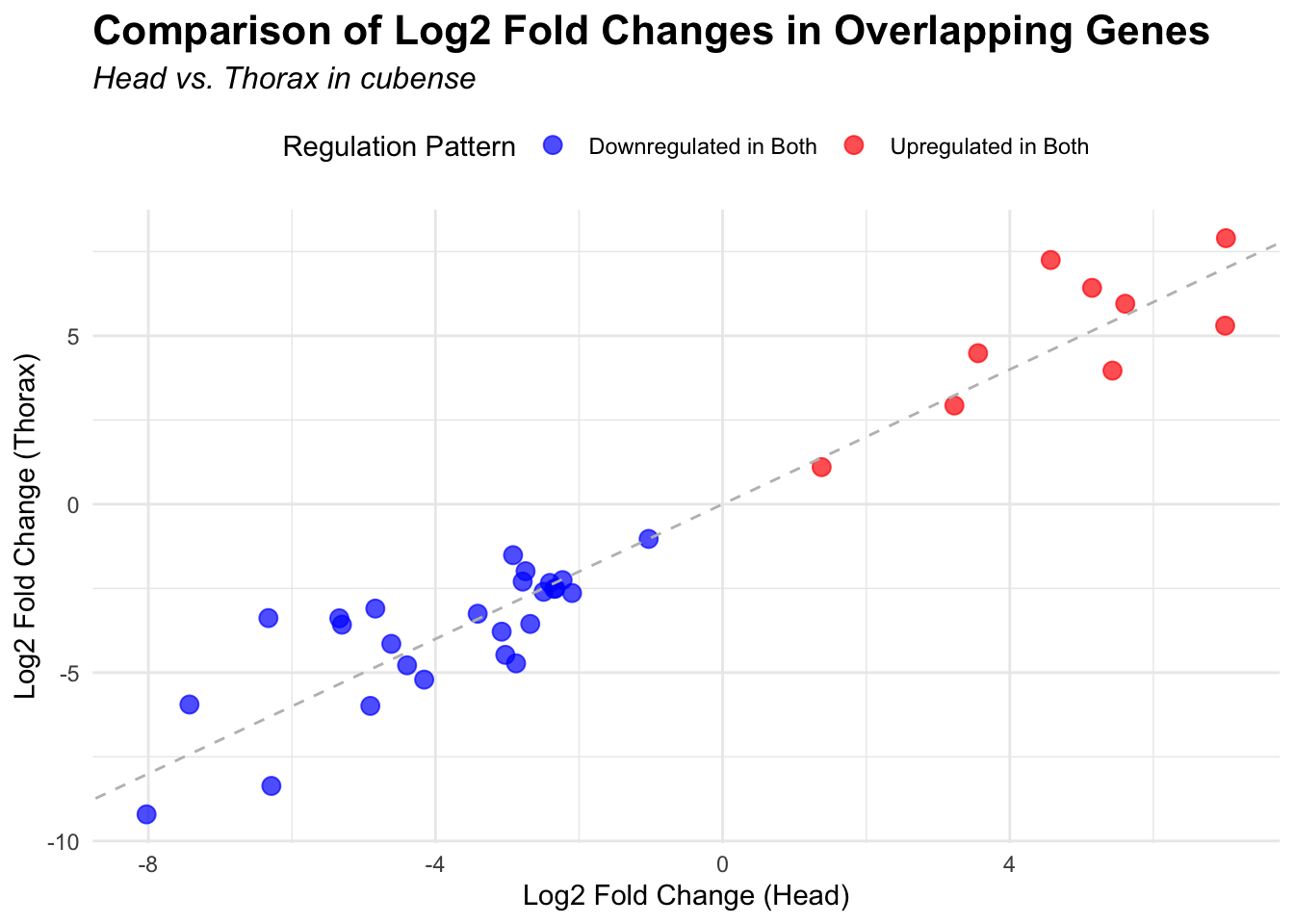
nitens
species <- "nitens"  # Specify the species for which to generate plots

# Load DESeq2 results for head and thorax
head_file <- file.path(workDir, "DEG_results/Bulk_RNAseq/", paste0(species, "/Head/DESeq2_results_Head_", species,".csv"))
thorax_file <- file.path(workDir, "DEG_results/Bulk_RNAseq/", paste0(species, "/Thorax/DESeq2_results_Thorax_", species,".csv"))

head_data <- read.csv(head_file, stringsAsFactors = FALSE)
thorax_data <- read.csv(thorax_file, stringsAsFactors = FALSE)

# Check if data is empty and handle accordingly
if (nrow(head_data) == 0 || nrow(thorax_data) == 0) {
    message(paste("No data for species:", species))
} else {
    # Filter for significant DEGs and select upregulated and downregulated genes
    head_up <- head_data %>%
        filter(padj < 0.05 & log2FoldChange > 1) %>%
        select(GeneID = X)

    head_down <- head_data %>%
        filter(padj < 0.05 & log2FoldChange < -1) %>%
        select(GeneID = X)

    thorax_up <- thorax_data %>%
        filter(padj < 0.05 & log2FoldChange > 1) %>%
        select(GeneID = X)

    thorax_down <- thorax_data %>%
        filter(padj < 0.05 & log2FoldChange < -1) %>%
        select(GeneID = X)

    # Prepare data for Venn diagram
    venn_data <- list(
        Head_Upregulated = head_up$GeneID,
        Head_Downregulated = head_down$GeneID,
        Thorax_Upregulated = thorax_up$GeneID,
        Thorax_Downregulated = thorax_down$GeneID
    )

    # Generate the four-way Venn diagram with specified colors and legend outside
    venn_plot <- venn.diagram(
        x = venn_data,
        category.names = c("Head Upregulated", "Head Downregulated", "Thorax Upregulated", "Thorax Downregulated"),
        filename = NULL,
        output = TRUE,
        fill = c("red", "skyblue", "orange", "blue"),  # Set colors for upregulated and downregulated
        alpha = 0.5,
        cex = 2,  # Text size for numbers
        cat.cex = 0,  # Text size for category labels
        cat.pos = c(0, 0, 0, 0),  # Position to center labels
        cat.dist = c(0.1, 0.1, 0.1, 0.1),  # Distance between category labels and circles
        main = paste("Venn Diagram of DEGs for S.", species),
        main.cex = 1.2,  # Size of the main title
        cat.col = c("red", "skyblue", "orange", "blue")  # Color the category labels
    )

    # Clear the current plotting area before drawing the next Venn diagram
    grid.newpage()

    # Display the Venn diagram
    grid.draw(venn_plot)

    # Manually create a custom legend
    legend_labels <- c("Head Up", "Head Down", "Thorax Up", "Thorax Down")
    legend_colors <- c("red", "skyblue", "orange", "blue")

    # Positioning the legend lower on the right side of the plot
    legend_x <- unit(0.85, "npc")  # Adjust x position
    legend_y <- unit(0.2, "npc")    # Lower the legend vertically

    # Draw the legend
    for (i in 1:length(legend_labels)) {
        grid.rect(x = legend_x, y = legend_y - unit((i - 1) * 0.05, "npc"),
                  width = unit(0.02, "npc"), height = unit(0.02, "npc"),
                  gp = gpar(fill = legend_colors[i], col = NA))
        grid.text(label = legend_labels[i], x = legend_x + unit(0.05, "npc"),
                  y = legend_y - unit((i - 1) * 0.05, "npc"),
                  just = "left", gp = gpar(cex = 0.8))
    }

    # Scatter plot for overlapping genes
    # Filter significant DEGs for both head and thorax
    head_sig_genes <- head_data %>%
        filter(padj < 0.05 & abs(log2FoldChange) > 1) %>%
        select(GeneID = X, log2FoldChange, padj)

    thorax_sig_genes <- thorax_data %>%
        filter(padj < 0.05 & abs(log2FoldChange) > 1) %>%
        select(GeneID = X, log2FoldChange, padj)

    # Find overlapping genes based on GeneID
    overlapping_genes <- inner_join(head_sig_genes, thorax_sig_genes, by = "GeneID", suffix = c("_head", "_thorax"))

    # Save the overlapping genes to a CSV file
    output_file <- file.path(workDir, "overlap/Bulk_RNAseq", paste0("overlapping_genes_head_thorax_", species, ".csv"))
    write.csv(overlapping_genes, output_file, row.names = FALSE)

    # Plot overlapping genes with scatter plot
    p <- ggplot(overlapping_genes, aes(x = log2FoldChange_head, y = log2FoldChange_thorax)) +
        geom_point(aes(color = case_when(
            log2FoldChange_head > 0 & log2FoldChange_thorax > 0 ~ "Upregulated in Both",
            log2FoldChange_head < 0 & log2FoldChange_thorax < 0 ~ "Downregulated in Both",
            log2FoldChange_head > 0 & log2FoldChange_thorax < 0 ~ "Up in Head, Down in Thorax",
            log2FoldChange_head < 0 & log2FoldChange_thorax > 0 ~ "Down in Head, Up in Thorax"
        )), size = 3, alpha = 0.7) +
        geom_abline(slope = 1, intercept = 0, linetype = "dashed", color = "gray") +
        labs(
            x = "Log2 Fold Change (Head)",
            y = "Log2 Fold Change (Thorax)",
            color = "Regulation Pattern",
            title = "Comparison of Log2 Fold Changes in Overlapping Genes",
            subtitle = paste("Head vs. Thorax in", species)
        ) +
        theme_minimal() +
        theme(
            plot.title = element_text(size = 16, face = "bold"),
            plot.subtitle = element_text(size = 12, face = "italic"),
            legend.position = "top"
        ) +
        scale_color_manual(values = c(
            "Upregulated in Both" = "red",
            "Downregulated in Both" = "blue",
            "Up in Head, Down in Thorax" = "purple",
            "Down in Head, Up in Thorax" = "green"
        ))

    # Save the scatter plot
    ggsave(filename = file.path(workDir, "overlap/Bulk_RNAseq", paste0("scatter_plot_overlapping_genes_", species, ".png")), plot = p)

    # Display the scatter plot
    print(p)
}
3. Overlap DEGs among species
Locusts
Head tissues
# Define the species for Group 1
locusts <- c("gregaria", "piceifrons", "cancellata")
input_file <- file.path(ortho_dir, "Results_I2/Orthogroups_genesproteinbiotype_Schistocerca_Jan2025.csv")
filtered_final_orthotable <- read.csv(input_file, header = TRUE, stringsAsFactors = FALSE)

# Function to load DEGs for a given group of species
load_deg_data <- function(locusts, allspecies_df, filtered_final_orthotable) {
    degs_up <- list()
    degs_down <- list()
    degs_all <- list()

    # Rename the "gene_id" column in filtered_final_orthotable for consistency
    #colnames(filtered_final_orthotable)[colnames(filtered_final_orthotable) == "gene_id"] <- "GeneID"

    for (species in locusts) {
        head_file <- file.path(workDir, "DEG_results/Bulk_RNAseq/", paste0(species, "/Head/DESeq2_results_Head_", species,".csv"))

        # Check if the file exists
        if (!file.exists(head_file)) {
            message(paste("File not found for species:", species))
            next  # Skip this iteration if the file is missing
        }

        # Read the data
        head_data <- read.csv(head_file, stringsAsFactors = FALSE)

        # Rename the "X" column to "GeneID"
        #colnames(head_data)[colnames(head_data) == "X"] <- "GeneID"

        # Merge DEG data with GeneType and Orthogroup information
        head_data_merged <- merge(head_data, allspecies_df[, c("GeneID", "GeneType", "Species")], by = "GeneID")
        head_data_merged <- merge(head_data_merged, filtered_final_orthotable[, c("GeneID", "Orthogroup")], by = "GeneID")

        # Handle missing Orthogroups
        head_data_merged$Orthogroup[is.na(head_data_merged$Orthogroup)] <- "Unknown"

        # Filter for significant DEGs (both upregulated and downregulated)
        head_up <- head_data_merged %>%
            filter(padj < 0.05 & log2FoldChange >= 1) %>%
            select(Orthogroup) %>%
            distinct()

        head_down <- head_data_merged %>%
            filter(padj < 0.05 & log2FoldChange <= -1) %>%
            select(Orthogroup) %>%
            distinct()

        all_deg <- head_data_merged %>%
            filter(padj < 0.05 & abs(log2FoldChange) >= 1) %>%
            select(Orthogroup) %>%
            distinct()

        # Store the DEGs in the list
        degs_up[[species]] <- head_up$Orthogroup
        degs_down[[species]] <- head_down$Orthogroup
        degs_all[[species]] <- all_deg$Orthogroup
    }

    return(list(up = degs_up, down = degs_down, all = degs_all))
}

# Function to display Venn diagram and corresponding datatable based on Orthogroups
display_venn_with_datatable <- function(venn_data, title, allspecies_df, filtered_final_orthotable) {

    # Calculate overlapping Orthogroups
    overlap_orthogroups <- Reduce(intersect, venn_data)

    # Print overlap info
    cat("Overlapping Orthogroups: \n")
    print(overlap_orthogroups)

    # If no overlaps exist, display a message and an empty plot
    if (length(overlap_orthogroups) == 0) {
        message("⚠️ No overlapping Orthogroups found. Displaying an empty Venn diagram.")

        # Create an empty Venn diagram placeholder
        plot.new()
        text(0.5, 0.5, "No overlapping Orthogroups found", cex = 1.5, col = "red")

        return(NULL)  # Exit the function gracefully
    }

    # Create a data frame for the overlapping Orthogroups
    overlap_df <- data.frame(Orthogroup = overlap_orthogroups)

    # Merge to get species and other information from filtered_final_orthotable
    meta_brock_df <- merge(overlap_df, filtered_final_orthotable, by = "Orthogroup", all.x = TRUE)

    # Ensure merged data exists
    if (nrow(meta_brock_df) == 0) {
        message("⚠️ Merge failed: No matching rows after merging Orthogroups.")
        return(NULL)
    }

    # Generate the Venn diagram
    venn_plot <- venn.diagram(
        x = venn_data,
        category.names = c("gregaria", "piceifrons", "cancellata"),
        filename = NULL,
        output = TRUE,
        fill = c("orange", "red", "orchid"),
        alpha = 0.5,
        cex = 2,
        cat.cex = 0,
        main = title,
        main.cex = 1.2
    )

    # Clear the current plotting area before drawing the Venn diagram
    grid.newpage()

    # Display the Venn diagram
    grid.draw(venn_plot)

    # Display the datatable for overlapping Orthogroups
    datatable(meta_brock_df, options = list(
        pageLength = 10,
        scrollX = TRUE,
        autoWidth = TRUE,
        searchHighlight = TRUE
    ),
    rownames = FALSE,
    escape = FALSE
    ) %>%
        formatStyle(
            'Species', target = 'cell',
            fontStyle = 'italic'
        )
}

# Load DEGs for locusts
venn_data_locusts <- load_deg_data(locusts, allspecies_df, filtered_final_orthotable)

# Prepare the data for Venn diagrams
venn_data_up <- list(
  gregaria = venn_data_locusts$up[["gregaria"]],
  piceifrons = venn_data_locusts$up[["piceifrons"]],
  cancellata = venn_data_locusts$up[["cancellata"]]
)

venn_data_down <- list(
  gregaria = venn_data_locusts$down[["gregaria"]],
  piceifrons = venn_data_locusts$down[["piceifrons"]],
  cancellata = venn_data_locusts$down[["cancellata"]]
)

venn_data_all <- list(
  gregaria = venn_data_locusts$all[["gregaria"]],
  piceifrons = venn_data_locusts$all[["piceifrons"]],
  cancellata = venn_data_locusts$all[["cancellata"]]
)

# Display the Venn diagrams with fallback for missing overlaps
message("Processing Venn diagram for head upregulated DEGs...")
display_venn_with_datatable(venn_data_up, "Venn Diagram of Head Upregulated DEGs - Locusts", allspecies_df, filtered_final_orthotable)
Overlapping Orthogroups:
[1] "Unknown" "OG0013490" "OG0007485" "OG0004381" "OG0000630" "OG0008668"
[7] "OG0000522" "OG0000307" "OG0000354" "OG0009529" "OG0000197" "OG0010634"
[13] "OG0000447" "OG0010928" "OG0005151" "OG0001019" "OG0000272"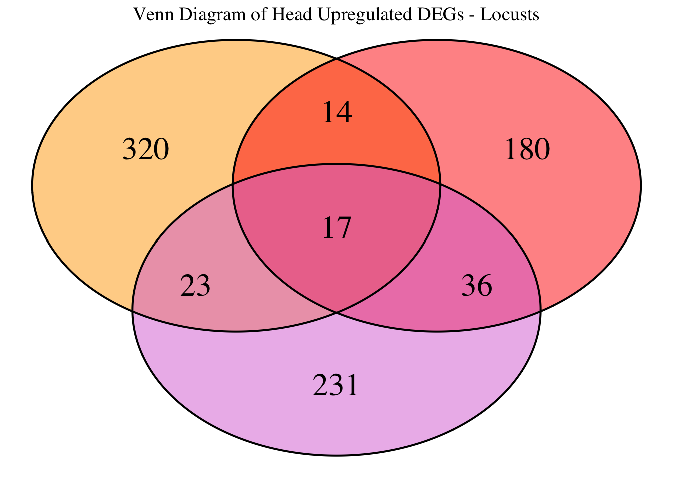
message("Processing Venn diagram for head downregulated DEGs...")
display_venn_with_datatable(venn_data_down, "Venn Diagram of Head Downregulated DEGs - Locusts", allspecies_df, filtered_final_orthotable)
Overlapping Orthogroups:
[1] "Unknown" "OG0012948" "OG0008546" "OG0014256" "OG0004570" "OG0009787"
[7] "OG0013175" "OG0010889" "OG0011171" "OG0000270" "OG0002151" "OG0003935"
[13] "OG0000505" "OG0000273" "OG0000149"
message("Processing Venn diagram for all significant DEGs...")
display_venn_with_datatable(venn_data_all, "Venn Diagram of All Head DEGs - Locusts", allspecies_df, filtered_final_orthotable)
Overlapping Orthogroups:
[1] "Unknown" "OG0013490" "OG0007485" "OG0004381" "OG0000630" "OG0012948"
[7] "OG0008668" "OG0008546" "OG0000522" "OG0008322" "OG0000307" "OG0014256"
[13] "OG0000354" "OG0004570" "OG0009537" "OG0009529" "OG0000197" "OG0009787"
[19] "OG0010634" "OG0013175" "OG0010889" "OG0000447" "OG0010928" "OG0011171"
[25] "OG0005490" "OG0000270" "OG0005151" "OG0001019" "OG0002151" "OG0003935"
[31] "OG0000272" "OG0000505" "OG0000273" "OG0000149"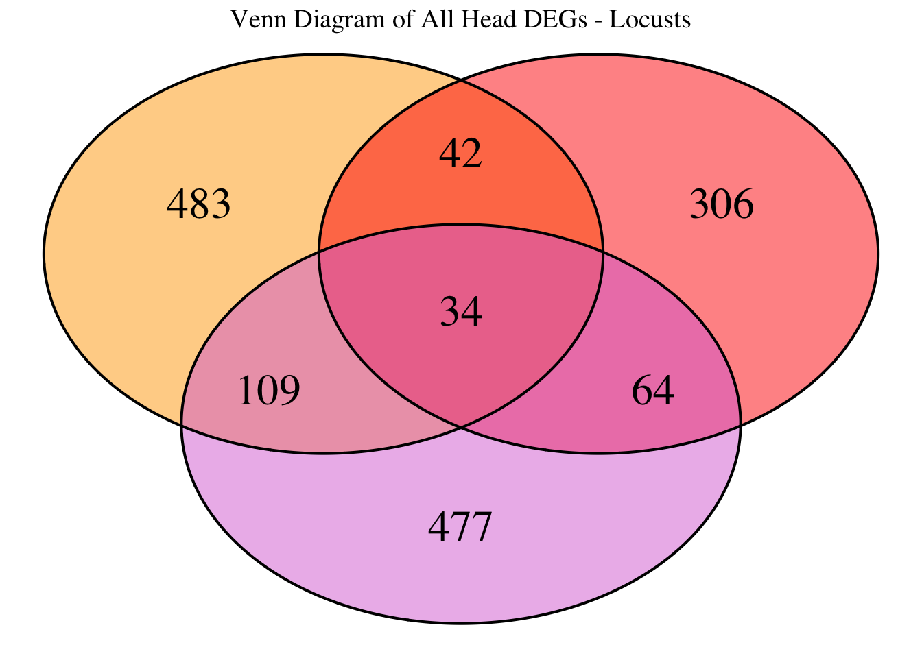
# Define the species for Group 1
locusts <- c("gregaria", "piceifrons", "cancellata")
input_file <- file.path(ortho_dir, "Results_I2/Orthogroups_genesproteinbiotype_Schistocerca_Jan2025.csv")
filtered_final_orthotable <- read.csv(input_file, header = TRUE, stringsAsFactors = FALSE)
# Initialize an empty list to store heatmap data for each species
heatmap_list <- list()

# Loop through each species to process their data
for (species in locusts) {
  # Load DESeq2 results for head
  head_file <- file.path(workDir, "DEG_results/Bulk_RNAseq/", paste0(species, "/Head/DESeq2_results_Head_", species,".csv"))

  # Load the DESeq2 results
  head_data <- read.csv(head_file, stringsAsFactors = FALSE)

  # Check if data is empty and handle accordingly
  if (nrow(head_data) == 0) {
    message(paste("No data for species:", species))
    next  # Skip to the next species if there's no data
  }

  # Rename the "gene_id" column in filtered_final_orthotable for consistency
  #colnames(filtered_final_orthotable)[colnames(filtered_final_orthotable) == "gene_id"] <- "GeneID"

  # Merge with filtered_final_orthotable to include Orthogroup
  merged_data <- merge(head_data, filtered_final_orthotable, by = "GeneID", all.x = TRUE)

  # Check if merge was successful
  if (nrow(merged_data) == 0) {
    message(paste("No matching data for species:", species))
    next  # Skip if no matching data after merging
  }

  # Filter for significant DEGs and select top 500 upregulated and downregulated genes for each tissue
  head_up <- merged_data %>%
    filter(padj < 0.05 & log2FoldChange > 1) %>%
    arrange(desc(log2FoldChange)) %>%
    slice(1:500)

  head_down <- merged_data %>%
    filter(padj < 0.05 & log2FoldChange < -1) %>%
    arrange(log2FoldChange) %>%
    slice(1:500)

  # Combine data and prepare for heatmap, adding the species column
  heatmap_data <- bind_rows(
    head_up %>% mutate(Tissue = "Head", Regulation = "Upregulated", Species = species),
    head_down %>% mutate(Tissue = "Head", Regulation = "Downregulated", Species = species)
  ) %>%
    select(Orthogroup, log2FoldChange, Tissue, Regulation, Species)

  # Append the heatmap data to the list
  heatmap_list[[species]] <- heatmap_data
}

# Combine all species data into a single dataframe for heatmap matrix preparation
final_heatmap_data <- bind_rows(heatmap_list)

# Check if final_heatmap_data is empty before proceeding
if (nrow(final_heatmap_data) == 0) {
    stop("No valid data available for heatmap generation.")
}

# Filter out rows with missing Orthogroup values
final_heatmap_data <- final_heatmap_data %>%
    filter(!is.na(Orthogroup))

# Check if there are any missing values in log2FoldChange (optional, just in case)
final_heatmap_data <- final_heatmap_data %>%
    filter(!is.na(log2FoldChange))

# Create heatmap matrix using Orthogroup instead of GeneID
heatmap_matrix <- final_heatmap_data %>%
    group_by(Orthogroup, Species) %>%
    summarize(
        Head_Combined = sum(log2FoldChange[Tissue == "Head"], na.rm = TRUE),
        .groups = 'drop'
    ) %>%
    pivot_wider(names_from = Species,
                values_from = Head_Combined,
                values_fill = list(Head_Combined = 0)) %>%
    column_to_rownames("Orthogroup") %>%
    as.matrix()

# Check if heatmap_matrix is empty
if (nrow(heatmap_matrix) == 0) {
    stop("No valid data available for heatmap matrix.")
}

# Define color palettes
# Define a custom color gradient where 0 is black
custom_color_palette1 <- colorRampPalette(c("cyan", "cyan3", "black", "orange3", "orange"))(100)

# Define a custom color gradient where 0 is white
custom_color_palette2 <- colorRampPalette(c("blue3", "blue", "white", "red", "red3"))(100)

# Define color breaks so that black is exactly at 0
max_abs_lfc <- max(abs(heatmap_matrix), na.rm = TRUE)  # Get max absolute log2FoldChange
color_breaks <- seq(-max_abs_lfc, max_abs_lfc, length.out = 100)  # Symmetric scale

# Create heatmap with clustering
pheatmap(
  heatmap_matrix,
  color = custom_color_palette2,
  breaks = color_breaks,
  cluster_rows = TRUE,  # Cluster genes
  cluster_cols = FALSE,  # Do not cluster species
  show_rownames = FALSE,
  show_colnames = TRUE,
  fontsize_row = 6,
  fontsize_col = 10,
  main = "Heatmap of Orthologs Expression in Head Tissue - STRATEGY 2"
)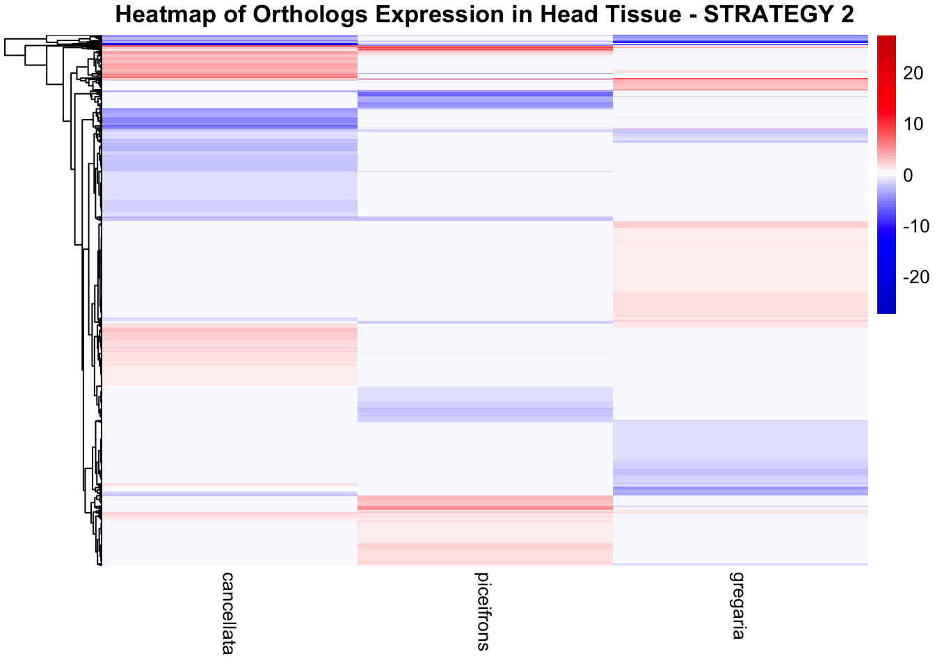
# Create heatmap without clustering columns
pheatmap(
  heatmap_matrix,
  color = custom_color_palette1,
  breaks = color_breaks,
  cluster_rows = TRUE,
  cluster_cols = FALSE,
  show_rownames = FALSE,
  show_colnames = TRUE,
  fontsize_row = 6,
  fontsize_col = 10,
  main = "Heatmap of Orthologs Expression in Head Tissue - STRATEGY 2"
)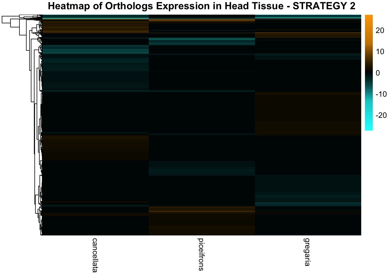
Thorax tissues
# Define the species for Group 1
locusts <- c("gregaria", "piceifrons", "cancellata")
input_file <- file.path(ortho_dir, "Results_I2/Orthogroups_genesproteinbiotype_Schistocerca_Jan2025.csv")
filtered_final_orthotable <- read.csv(input_file, header = TRUE, stringsAsFactors = FALSE)

# Function to load DEGs for a given group of species
load_deg_data <- function(locusts, allspecies_df, filtered_final_orthotable) {
    degs_up <- list()
    degs_down <- list()
    degs_all <- list()

    # Rename the "gene_id" column in filtered_final_orthotable for consistency
    #colnames(filtered_final_orthotable)[colnames(filtered_final_orthotable) == "gene_id"] <- "GeneID"

    for (species in locusts) {
        thorax_file <- file.path(workDir, "DEG_results/Bulk_RNAseq/", paste0(species, "/Thorax/DESeq2_results_Thorax_", species,".csv"))

        # Check if the file exists
        if (!file.exists(thorax_file)) {
            message(paste("File not found for species:", species))
            next  # Skip this iteration if the file is missing
        }

        # Read the data
        thorax_data <- read.csv(thorax_file, stringsAsFactors = FALSE)

        # Rename the "X" column to "GeneID"
        #colnames(thorax_data)[colnames(thorax_data) == "X"] <- "GeneID"

        # Merge DEG data with GeneType and Orthogroup information
        thorax_data_merged <- merge(thorax_data, allspecies_df[, c("GeneID", "GeneType", "Species")], by = "GeneID")
        thorax_data_merged <- merge(thorax_data_merged, filtered_final_orthotable[, c("GeneID", "Orthogroup")], by = "GeneID")

        # Handle missing Orthogroups
        thorax_data_merged$Orthogroup[is.na(thorax_data_merged$Orthogroup)] <- "Unknown"

        # Filter for significant DEGs (both upregulated and downregulated)
        thorax_up <- thorax_data_merged %>%
            filter(padj < 0.05 & log2FoldChange >= 1) %>%
            select(Orthogroup) %>%
            distinct()

        thorax_down <- thorax_data_merged %>%
            filter(padj < 0.05 & log2FoldChange <= -1) %>%
            select(Orthogroup) %>%
            distinct()

        all_deg <- thorax_data_merged %>%
            filter(padj < 0.05 & abs(log2FoldChange) >= 1) %>%
            select(Orthogroup) %>%
            distinct()

        # Store the DEGs in the list
        degs_up[[species]] <- thorax_up$Orthogroup
        degs_down[[species]] <- thorax_down$Orthogroup
        degs_all[[species]] <- all_deg$Orthogroup
    }

    return(list(up = degs_up, down = degs_down, all = degs_all))
}

# Function to display Venn diagram and corresponding datatable based on Orthogroups
# Function to display Venn diagram and corresponding datatable
display_venn_with_datatable <- function(venn_data, title, allspecies_df, filtered_final_orthotable) {

    # Calculate overlapping Orthogroups
    overlap_orthogroups <- Reduce(intersect, venn_data)

    # Print overlap info
    cat("Overlapping Orthogroups: \n")
    print(overlap_orthogroups)

    # If no overlaps exist, display a message and an empty plot
    if (length(overlap_orthogroups) == 0) {
        message("⚠️ No overlapping Orthogroups found. Displaying an empty Venn diagram.")

        # Create an empty Venn diagram placeholder
        plot.new()
        text(0.5, 0.5, "No overlapping Orthogroups found", cex = 1.5, col = "red")

        return(NULL)  # Exit the function gracefully
    }

    # Create a data frame for the overlapping Orthogroups
    overlap_df <- data.frame(Orthogroup = overlap_orthogroups)

    # Merge to get species and other information from filtered_final_orthotable
    meta_brock_df <- merge(overlap_df, filtered_final_orthotable, by = "Orthogroup", all.x = TRUE)

    # Ensure merged data exists
    if (nrow(meta_brock_df) == 0) {
        message("⚠️ Merge failed: No matching rows after merging Orthogroups.")
        return(NULL)
    }

    # Generate the Venn diagram
    venn_plot <- venn.diagram(
        x = venn_data,
        category.names = c("gregaria", "piceifrons", "cancellata"),
        filename = NULL,
        output = TRUE,
        fill = c("orange", "red", "orchid"),
        alpha = 0.5,
        cex = 2,
        cat.cex = 0,
        main = title,
        main.cex = 1.2
    )

    # Clear the current plotting area before drawing the Venn diagram
    grid.newpage()

    # Display the Venn diagram
    grid.draw(venn_plot)

    # Display the datatable for overlapping Orthogroups
    datatable(meta_brock_df, options = list(
        pageLength = 10,
        scrollX = TRUE,
        autoWidth = TRUE,
        searchHighlight = TRUE
    ),
    rownames = FALSE,
    escape = FALSE
    ) %>%
        formatStyle(
            'Species', target = 'cell',
            fontStyle = 'italic'
        )
}

# Load DEGs for locusts
venn_data_locusts <- load_deg_data(locusts, allspecies_df, filtered_final_orthotable)

# Prepare the data for Venn diagrams
venn_data_up <- list(
  gregaria = venn_data_locusts$up[["gregaria"]],
  piceifrons = venn_data_locusts$up[["piceifrons"]],
  cancellata = venn_data_locusts$up[["cancellata"]]
)

venn_data_down <- list(
  gregaria = venn_data_locusts$down[["gregaria"]],
  piceifrons = venn_data_locusts$down[["piceifrons"]],
  cancellata = venn_data_locusts$down[["cancellata"]]
)

venn_data_all <- list(
  gregaria = venn_data_locusts$all[["gregaria"]],
  piceifrons = venn_data_locusts$all[["piceifrons"]],
  cancellata = venn_data_locusts$all[["cancellata"]]
)

# Display the Venn diagrams with fallback for missing overlaps
message("Processing Venn diagram for thorax upregulated DEGs...")
display_venn_with_datatable(venn_data_up, "Venn Diagram of Thorax Upregulated DEGs - Locusts", allspecies_df, filtered_final_orthotable)
Overlapping Orthogroups:
[1] "OG0007864" "Unknown" "OG0012855" "OG0004381" "OG0000630" "OG0008668"
[7] "OG0008773" "OG0000354" "OG0013891" "OG0002449" "OG0000196" "OG0004741"
[13] "OG0009529" "OG0009902" "OG0000197" "OG0010559" "OG0010743" "OG0011005"
[19] "OG0011869" "OG0005151" "OG0006295" "OG0006293" "OG0005991" "OG0003684"
[25] "OG0003702" "OG0003704" "OG0006530" "OG0006498" "OG0000112" "OG0007438"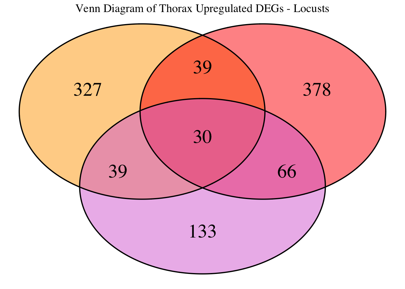
message("Processing Venn diagram for thorax downregulated DEGs...")
display_venn_with_datatable(venn_data_down, "Venn Diagram of Thorax Downregulated DEGs - Locusts", allspecies_df, filtered_final_orthotable)
Overlapping Orthogroups:
[1] "Unknown" "OG0014256" "OG0008629" "OG0008761" "OG0002570" "OG0009787"
[7] "OG0010410" "OG0011346" "OG0000270" "OG0003407" "OG0004972" "OG0000008"
[13] "OG0002151" "OG0000505"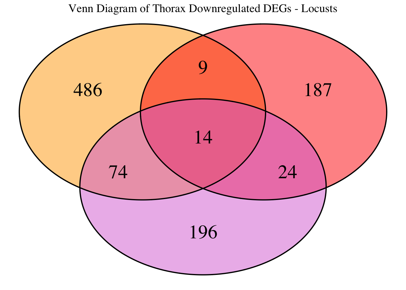
message("Processing Venn diagram for all significant DEGs...")
display_venn_with_datatable(venn_data_all, "Venn Diagram of All Thorax DEGs - Locusts", allspecies_df, filtered_final_orthotable)
Overlapping Orthogroups:
[1] "Unknown" "OG0007864" "OG0012855" "OG0004381" "OG0000630" "OG0008668"
[7] "OG0012943" "OG0014256" "OG0008773" "OG0000354" "OG0013891" "OG0008629"
[13] "OG0002449" "OG0008761" "OG0000196" "OG0002570" "OG0004741" "OG0000027"
[19] "OG0009529" "OG0009516" "OG0009902" "OG0000197" "OG0009787" "OG0002897"
[25] "OG0010559" "OG0010410" "OG0000446" "OG0010863" "OG0010743" "OG0011005"
[31] "OG0011162" "OG0011346" "OG0011869" "OG0001366" "OG0000396" "OG0000270"
[37] "OG0003407" "OG0005151" "OG0004972" "OG0014897" "OG0006295" "OG0006293"
[43] "OG0000008" "OG0005991" "OG0005943" "OG0012394" "OG0003684" "OG0003702"
[49] "OG0003704" "OG0006530" "OG0002151" "OG0000218" "OG0006498" "OG0000112"
[55] "OG0000505" "OG0000504" "OG0000037" "OG0007438"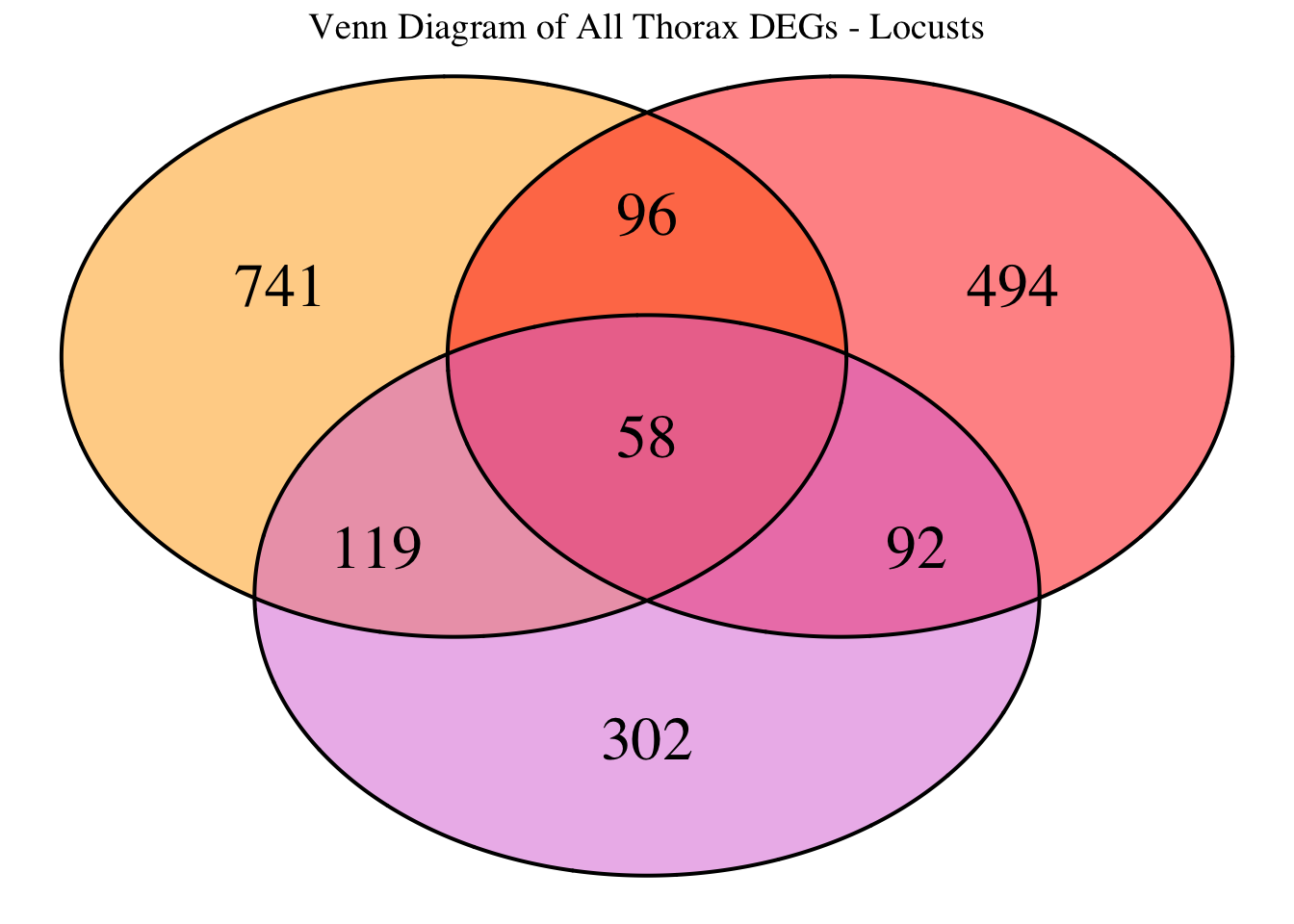
# Define the species for Group 1
locusts <- c("gregaria", "piceifrons", "cancellata")
input_file <- file.path(ortho_dir, "Results_I2/Orthogroups_genesproteinbiotype_Schistocerca_Jan2025.csv")
filtered_final_orthotable <- read.csv(input_file, header = TRUE, stringsAsFactors = FALSE)
# Initialize an empty list to store heatmap data for each species
heatmap_list <- list()

# Loop through each species to process their data
for (species in locusts) {
  # Load DESeq2 results for head
  thorax_file <- file.path(workDir, "DEG_results/Bulk_RNAseq/", paste0(species, "/Thorax/DESeq2_results_Thorax_", species,".csv"))

  # Load the DESeq2 results
  thorax_data <- read.csv(thorax_file, stringsAsFactors = FALSE)

  # Check if data is empty and handle accordingly
  if (nrow(thorax_data) == 0) {
    message(paste("No data for species:", species))
    next  # Skip to the next species if there's no data
  }

  # Rename the "gene_id" column in filtered_final_orthotable for consistency
  colnames(filtered_final_orthotable)[colnames(filtered_final_orthotable) == "gene_id"] <- "GeneID"

  # Merge with filtered_final_orthotable to include Orthogroup
  merged_data <- merge(thorax_data, filtered_final_orthotable, by = "GeneID", all.x = TRUE)

  # Check if merge was successful
  if (nrow(merged_data) == 0) {
    message(paste("No matching data for species:", species))
    next  # Skip if no matching data after merging
  }

  # Filter for significant DEGs and select top 500 upregulated and downregulated genes for each tissue
  thorax_up <- merged_data %>%
    filter(padj < 0.05 & log2FoldChange > 1) %>%
    arrange(desc(log2FoldChange)) %>%
    slice(1:500)

  thorax_down <- merged_data %>%
    filter(padj < 0.05 & log2FoldChange < -1) %>%
    arrange(log2FoldChange) %>%
    slice(1:500)

  # Combine data and prepare for heatmap, adding the species column
  heatmap_data <- bind_rows(
    thorax_up %>% mutate(Tissue = "Thorax", Regulation = "Upregulated", Species = species),
    thorax_down %>% mutate(Tissue = "Thorax", Regulation = "Downregulated", Species = species)
  ) %>%
    select(Orthogroup, log2FoldChange, Tissue, Regulation, Species)

  # Append the heatmap data to the list
  heatmap_list[[species]] <- heatmap_data
}

# Combine all species data into a single dataframe for heatmap matrix preparation
final_heatmap_data <- bind_rows(heatmap_list)

# Check if final_heatmap_data is empty before proceeding
if (nrow(final_heatmap_data) == 0) {
    stop("No valid data available for heatmap generation.")
}

# Filter out rows with missing Orthogroup values
final_heatmap_data <- final_heatmap_data %>%
    filter(!is.na(Orthogroup))

# Check if there are any missing values in log2FoldChange (optional, just in case)
final_heatmap_data <- final_heatmap_data %>%
    filter(!is.na(log2FoldChange))

# Create heatmap matrix using Orthogroup instead of GeneID
heatmap_matrix <- final_heatmap_data %>%
    group_by(Orthogroup, Species) %>%
    summarize(
        Thorax_Combined = sum(log2FoldChange[Tissue == "Thorax"], na.rm = TRUE),
        .groups = 'drop'
    ) %>%
    pivot_wider(names_from = Species,
                values_from = Thorax_Combined,
                values_fill = list(Thorax_Combined = 0)) %>%
    column_to_rownames("Orthogroup") %>%
    as.matrix()

# Check if heatmap_matrix is empty
if (nrow(heatmap_matrix) == 0) {
    stop("No valid data available for heatmap matrix.")
}

# Define color palettes
# Define a custom color gradient where 0 is black
custom_color_palette1 <- colorRampPalette(c("cyan", "cyan3", "black", "orange3", "orange"))(100)

# Define a custom color gradient where 0 is white
custom_color_palette2 <- colorRampPalette(c("blue3", "blue", "white", "red", "red3"))(100)

# Define color breaks so that black is exactly at 0
max_abs_lfc <- max(abs(heatmap_matrix), na.rm = TRUE)  # Get max absolute log2FoldChange
color_breaks <- seq(-max_abs_lfc, max_abs_lfc, length.out = 100)  # Symmetric scale

# Create heatmap with clustering
pheatmap(
  heatmap_matrix,
  color = custom_color_palette2,
  breaks = color_breaks,
  cluster_rows = TRUE,  # Cluster genes
  cluster_cols = FALSE,  # Do not cluster species
  show_rownames = FALSE,
  show_colnames = TRUE,
  fontsize_row = 6,
  fontsize_col = 10,
  main = "Heatmap of Orthologs Expression in Thorax Tissue - STRATEGY 2"
)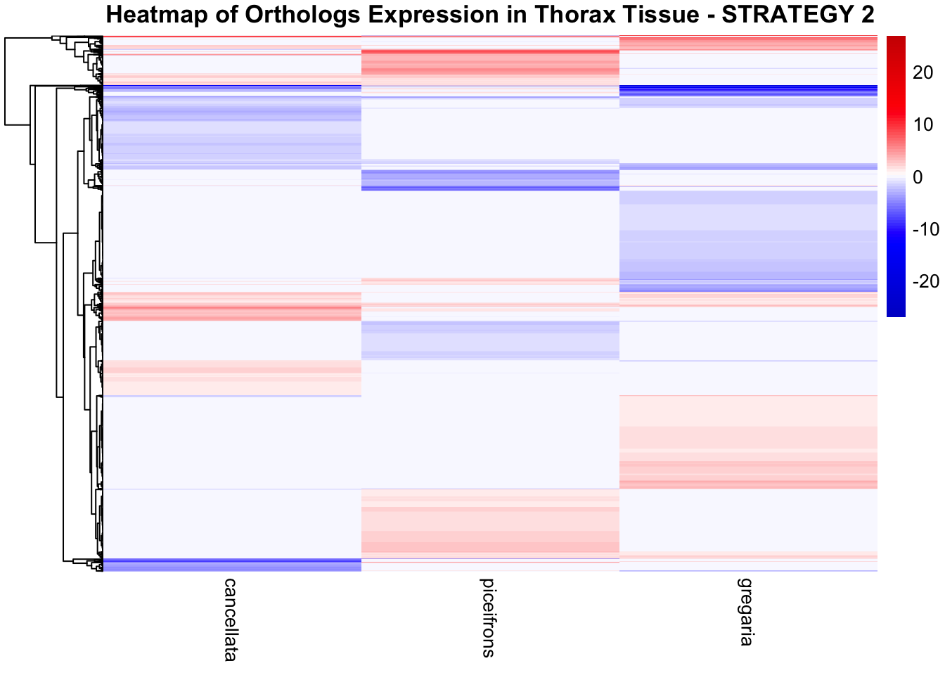
# Create heatmap without clustering columns
pheatmap(
  heatmap_matrix,
  color = custom_color_palette1,
  breaks = color_breaks,
  cluster_rows = TRUE,
  cluster_cols = FALSE,
  show_rownames = FALSE,
  show_colnames = TRUE,
  fontsize_row = 6,
  fontsize_col = 10,
  main = "Heatmap of Orthologs Expression in Thorax Tissue - STRATEGY 2"
)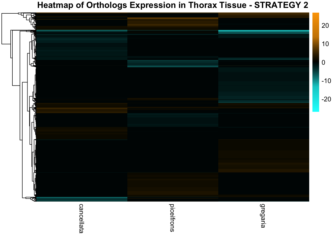
piceifrons-americana-cubense
Head tissues
# Define the species for PACclade
PACclade <- c("piceifrons", "americana", "cubense")
input_file <- file.path(ortho_dir, "Results_I2/Orthogroups_genesproteinbiotype_Schistocerca_Jan2025.csv")
filtered_final_orthotable <- read.csv(input_file, header = TRUE, stringsAsFactors = FALSE)

# Function to load DEGs for a given group of species
load_deg_data <- function(PACclade, allspecies_df, filtered_final_orthotable) {
    degs_up <- list()
    degs_down <- list()
    degs_all <- list()

    # Rename the "gene_id" column in filtered_final_orthotable for consistency
    colnames(filtered_final_orthotable)[colnames(filtered_final_orthotable) == "gene_id"] <- "GeneID"

    for (species in PACclade) {
        head_file <- file.path(workDir, "DEG_results/Bulk_RNAseq/", paste0(species, "/Head/DESeq2_results_Head_", species,".csv"))

        # Check if the file exists
        if (!file.exists(head_file)) {
            message(paste("File not found for species:", species))
            next  # Skip this iteration if the file is missing
        }

        # Read the data
        head_data <- read.csv(head_file, stringsAsFactors = FALSE)

        # Rename the "X" column to "GeneID"
        #colnames(head_data)[colnames(head_data) == "X"] <- "GeneID"

        # Merge DEG data with GeneType and Orthogroup information
        head_data_merged <- merge(head_data, allspecies_df[, c("GeneID", "GeneType", "Species")], by = "GeneID")
        head_data_merged <- merge(head_data_merged, filtered_final_orthotable[, c("GeneID", "Orthogroup")], by = "GeneID")

        # Handle missing Orthogroups
        head_data_merged$Orthogroup[is.na(head_data_merged$Orthogroup)] <- "Unknown"

        # Filter for significant DEGs (both upregulated and downregulated)
        head_up <- head_data_merged %>%
            filter(padj < 0.05 & log2FoldChange >= 1) %>%
            select(Orthogroup) %>%
            distinct()

        head_down <- head_data_merged %>%
            filter(padj < 0.05 & log2FoldChange <= -1) %>%
            select(Orthogroup) %>%
            distinct()

        all_deg <- head_data_merged %>%
            filter(padj < 0.05 & abs(log2FoldChange) >= 1) %>%
            select(Orthogroup) %>%
            distinct()

        # Store the DEGs in the list
        degs_up[[species]] <- head_up$Orthogroup
        degs_down[[species]] <- head_down$Orthogroup
        degs_all[[species]] <- all_deg$Orthogroup
    }

    return(list(up = degs_up, down = degs_down, all = degs_all))
}

# Function to display Venn diagram and corresponding datatable based on Orthogroups
# Function to display Venn diagram and corresponding datatable
display_venn_with_datatable <- function(venn_data, title, allspecies_df, filtered_final_orthotable) {

    # Calculate overlapping Orthogroups
    overlap_orthogroups <- Reduce(intersect, venn_data)

    # Print overlap info
    cat("Overlapping Orthogroups: \n")
    print(overlap_orthogroups)

    # If no overlaps exist, display a message and an empty plot
    if (length(overlap_orthogroups) == 0) {
        message("⚠️ No overlapping Orthogroups found. Displaying an empty Venn diagram.")

        # Create an empty Venn diagram placeholder
        plot.new()
        text(0.5, 0.5, "No overlapping Orthogroups found", cex = 1.5, col = "red")

        return(NULL)  # Exit the function gracefully
    }

    # Create a data frame for the overlapping Orthogroups
    overlap_df <- data.frame(Orthogroup = overlap_orthogroups)

    # Merge to get species and other information from filtered_final_orthotable
    meta_brock_df <- merge(overlap_df, filtered_final_orthotable, by = "Orthogroup", all.x = TRUE)

    # Ensure merged data exists
    if (nrow(meta_brock_df) == 0) {
        message("⚠️ Merge failed: No matching rows after merging Orthogroups.")
        return(NULL)
    }

    # Generate the Venn diagram
    venn_plot <- venn.diagram(
        x = venn_data,
        category.names = c("piceifrons", "americana", "cubense"),
        filename = NULL,
        output = TRUE,
        fill = c("red", "green", "yellow"),
        alpha = 0.5,
        cex = 2,
        cat.cex = 0,
        main = title,
        main.cex = 1.2
    )

    # Clear the current plotting area before drawing the Venn diagram
    grid.newpage()

    # Display the Venn diagram
    grid.draw(venn_plot)

    # Manually create a custom legend
    legend_labels <- c("piceifrons", "americana", "cubense")
    legend_colors <- c("red", "green", "yellow")

    # Positioning the legend lower on the right side of the plot
    legend_x <- unit(0.85, "npc")  # Adjust x position
    legend_y <- unit(0.2, "npc")   # Lower the legend vertically

    # Draw the legend
    for (i in 1:length(legend_labels)) {
        grid.rect(x = legend_x, y = legend_y - unit((i - 1) * 0.05, "npc"),
                  width = unit(0.02, "npc"), height = unit(0.02, "npc"),
                  gp = gpar(fill = legend_colors[i], col = NA))
        grid.text(label = legend_labels[i], x = legend_x + unit(0.05, "npc"),
                  y = legend_y - unit((i - 1) * 0.05, "npc"),
                  just = "left", gp = gpar(cex = 0.8))
    }

    # Display the merged overlapping Orthogroups table with datatable
    datatable(meta_brock_df, options = list(
        pageLength = 10,
        scrollX = TRUE,
        autoWidth = TRUE,
        searchHighlight = TRUE
    ),
    rownames = FALSE,
    escape = FALSE
    ) %>%
        formatStyle(
            'Species', target = 'cell',
            fontStyle = 'italic'
        ) %>%
        formatStyle(
            columns = names(meta_brock_df),
            target = 'row',
            color = styleEqual(c("red", "blue", "black"), c("red", "blue", "black")),
            fontWeight = styleEqual(c("bold", "normal"), c("bold", "normal")),
            backgroundColor = styleEqual(c("red", "blue", "black"), c("white", "white", "white"))
        )
}

# Example for testing with your data (for PACclade)
venn_data_pacclade <- load_deg_data(PACclade, allspecies_df, filtered_final_orthotable)

# Prepare the data for the Venn diagrams for PACclade
venn_data_up <- list(
  piceifrons = venn_data_pacclade$up[["piceifrons"]],
  americana = venn_data_pacclade$up[["americana"]],
  cubense = venn_data_pacclade$up[["cubense"]]
)

venn_data_down <- list(
  piceifrons = venn_data_pacclade$down[["piceifrons"]],
  americana = venn_data_pacclade$down[["americana"]],
  cubense = venn_data_pacclade$down[["cubense"]]
)

venn_data_all <- list(
  piceifrons = venn_data_pacclade$all[["piceifrons"]],
  americana = venn_data_pacclade$all[["americana"]],
  cubense = venn_data_pacclade$all[["cubense"]]
)

# Display the Venn diagram and datatable for head upregulated DEGs (PACclade)
display_venn_with_datatable(venn_data_up, "Venn Diagram of Head Upregulated DEGs - PAC", allspecies_df, filtered_final_orthotable)
Overlapping Orthogroups:
[1] "Unknown" "OG0006291" "OG0012596"
# Display the Venn diagram and datatable for head downregulated DEGs (PACclade)
display_venn_with_datatable(venn_data_down, "Venn Diagram of Head Downregulated DEGs - PAC", allspecies_df, filtered_final_orthotable)
Overlapping Orthogroups:
[1] "Unknown"
# Display the Venn diagram and datatable for all significant DEGs (PACclade)
display_venn_with_datatable(venn_data_all, "Venn Diagram of All Head DEGs - PAC", allspecies_df, filtered_final_orthotable)
Overlapping Orthogroups:
[1] "Unknown" "OG0006291" "OG0012596" "OG0008500"
# Define the species for Group 1
PACclade <- c("piceifrons", "americana", "cubense")
input_file <- file.path(ortho_dir, "Results_I2/Orthogroups_genesproteinbiotype_Schistocerca_Jan2025.csv")
filtered_final_orthotable <- read.csv(input_file, header = TRUE, stringsAsFactors = FALSE)
# Initialize an empty list to store heatmap data for each species
heatmap_list <- list()

# Loop through each species to process their data
for (species in PACclade) {
  # Load DESeq2 results for head
  head_file <- file.path(workDir, "DEG_results/Bulk_RNAseq/", paste0(species, "/Head/DESeq2_results_Head_", species,".csv"))

  # Load the DESeq2 results
  head_data <- read.csv(head_file, stringsAsFactors = FALSE)

  # Check if data is empty and handle accordingly
  if (nrow(head_data) == 0) {
    message(paste("No data for species:", species))
    next  # Skip to the next species if there's no data
  }

  # Rename the "gene_id" column in filtered_final_orthotable for consistency
  #colnames(filtered_final_orthotable)[colnames(filtered_final_orthotable) == "gene_id"] <- "GeneID"

  # Merge with filtered_final_orthotable to include Orthogroup
  merged_data <- merge(head_data, filtered_final_orthotable, by = "GeneID", all.x = TRUE)

  # Check if merge was successful
  if (nrow(merged_data) == 0) {
    message(paste("No matching data for species:", species))
    next  # Skip if no matching data after merging
  }

  # Filter for significant DEGs and select top 500 upregulated and downregulated genes for each tissue
  head_up <- merged_data %>%
    filter(padj < 0.05 & log2FoldChange > 1) %>%
    arrange(desc(log2FoldChange)) %>%
    slice(1:500)

  head_down <- merged_data %>%
    filter(padj < 0.05 & log2FoldChange < -1) %>%
    arrange(log2FoldChange) %>%
    slice(1:500)

  # Combine data and prepare for heatmap, adding the species column
  heatmap_data <- bind_rows(
    head_up %>% mutate(Tissue = "Head", Regulation = "Upregulated", Species = species),
    head_down %>% mutate(Tissue = "Head", Regulation = "Downregulated", Species = species)
  ) %>%
    select(Orthogroup, log2FoldChange, Tissue, Regulation, Species)

  # Append the heatmap data to the list
  heatmap_list[[species]] <- heatmap_data
}

# Combine all species data into a single dataframe for heatmap matrix preparation
final_heatmap_data <- bind_rows(heatmap_list)

# Check if final_heatmap_data is empty before proceeding
if (nrow(final_heatmap_data) == 0) {
    stop("No valid data available for heatmap generation.")
}

# Filter out rows with missing Orthogroup values
final_heatmap_data <- final_heatmap_data %>%
    filter(!is.na(Orthogroup))

# Check if there are any missing values in log2FoldChange (optional, just in case)
final_heatmap_data <- final_heatmap_data %>%
    filter(!is.na(log2FoldChange))

# Create heatmap matrix using Orthogroup instead of GeneID
heatmap_matrix <- final_heatmap_data %>%
    group_by(Orthogroup, Species) %>%
    summarize(
        Head_Combined = sum(log2FoldChange[Tissue == "Head"], na.rm = TRUE),
        .groups = 'drop'
    ) %>%
    pivot_wider(names_from = Species,
                values_from = Head_Combined,
                values_fill = list(Head_Combined = 0)) %>%
    column_to_rownames("Orthogroup") %>%
    as.matrix()

# Check if heatmap_matrix is empty
if (nrow(heatmap_matrix) == 0) {
    stop("No valid data available for heatmap matrix.")
}

# Define color palettes
# Define a custom color gradient where 0 is black
custom_color_palette1 <- colorRampPalette(c("cyan", "cyan3", "black", "orange3", "orange"))(100)

# Define a custom color gradient where 0 is white
custom_color_palette2 <- colorRampPalette(c("blue3", "blue", "white", "red", "red3"))(100)

# Define color breaks so that black is exactly at 0
max_abs_lfc <- max(abs(heatmap_matrix), na.rm = TRUE)  # Get max absolute log2FoldChange
color_breaks <- seq(-max_abs_lfc, max_abs_lfc, length.out = 100)  # Symmetric scale

# Create heatmap with clustering
pheatmap(
  heatmap_matrix,
  color = custom_color_palette2,
  breaks = color_breaks,
  cluster_rows = TRUE,  # Cluster genes
  cluster_cols = FALSE,  # Do not cluster species
  show_rownames = FALSE,
  show_colnames = TRUE,
  fontsize_row = 6,
  fontsize_col = 10,
  main = "Heatmap of Orthologs Expression in Head Tissue - STRATEGY 2"
)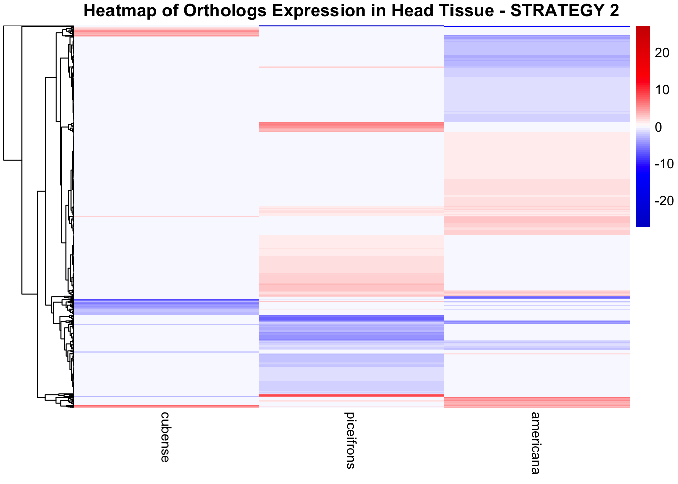
# Create heatmap without clustering columns
pheatmap(
  heatmap_matrix,
  color = custom_color_palette1,
  breaks = color_breaks,
  cluster_rows = TRUE,
  cluster_cols = FALSE,
  show_rownames = FALSE,
  show_colnames = TRUE,
  fontsize_row = 6,
  fontsize_col = 10,
  main = "Heatmap of Orthologs Expression in Head Tissue - STRATEGY 2"
)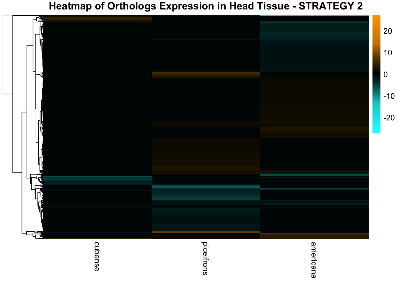
Thorax tissues
# Define the species for PACclade
PACclade <- c("piceifrons", "americana", "cubense")
input_file <- file.path(ortho_dir, "Results_I2/Orthogroups_genesproteinbiotype_Schistocerca_Jan2025.csv")
filtered_final_orthotable <- read.csv(input_file, header = TRUE, stringsAsFactors = FALSE)

# Function to load DEGs for a given group of species
load_deg_data <- function(PACclade, allspecies_df, filtered_final_orthotable) {
    degs_up <- list()
    degs_down <- list()
    degs_all <- list()

    # Rename the "gene_id" column in filtered_final_orthotable for consistency
    colnames(filtered_final_orthotable)[colnames(filtered_final_orthotable) == "gene_id"] <- "GeneID"

    for (species in PACclade) {
        thorax_file <- file.path(workDir, "DEG_results/Bulk_RNAseq/", paste0(species, "/Thorax/DESeq2_results_Thorax_", species,".csv"))

        # Check if the file exists
        if (!file.exists(thorax_file)) {
            message(paste("File not found for species:", species))
            next  # Skip this iteration if the file is missing
        }

        # Read the data
        thorax_data <- read.csv(thorax_file, stringsAsFactors = FALSE)

        # Rename the "X" column to "GeneID"
        #colnames(thorax_data)[colnames(thorax_data) == "X"] <- "GeneID"

        # Merge DEG data with GeneType and Orthogroup information
        thorax_data_merged <- merge(thorax_data, allspecies_df[, c("GeneID", "GeneType", "Species")], by = "GeneID")
        thorax_data_merged <- merge(thorax_data_merged, filtered_final_orthotable[, c("GeneID", "Orthogroup")], by = "GeneID")

        # Handle missing Orthogroups
        thorax_data_merged$Orthogroup[is.na(thorax_data_merged$Orthogroup)] <- "Unknown"

        # Filter for significant DEGs (both upregulated and downregulated)
        thorax_up <- thorax_data_merged %>%
            filter(padj < 0.05 & log2FoldChange >= 1) %>%
            select(Orthogroup) %>%
            distinct()

        thorax_down <- thorax_data_merged %>%
            filter(padj < 0.05 & log2FoldChange <= -1) %>%
            select(Orthogroup) %>%
            distinct()

        all_deg <- thorax_data_merged %>%
            filter(padj < 0.05 & abs(log2FoldChange) >= 1) %>%
            select(Orthogroup) %>%
            distinct()

        # Store the DEGs in the list
        degs_up[[species]] <- thorax_up$Orthogroup
        degs_down[[species]] <- thorax_down$Orthogroup
        degs_all[[species]] <- all_deg$Orthogroup
    }

    return(list(up = degs_up, down = degs_down, all = degs_all))
}

# Function to display Venn diagram and corresponding datatable based on Orthogroups
# Function to display Venn diagram and corresponding datatable
display_venn_with_datatable <- function(venn_data, title, allspecies_df, filtered_final_orthotable) {

    # Calculate overlapping Orthogroups
    overlap_orthogroups <- Reduce(intersect, venn_data)

    # Print overlap info
    cat("Overlapping Orthogroups: \n")
    print(overlap_orthogroups)

    # If no overlaps exist, display a message and an empty plot
    if (length(overlap_orthogroups) == 0) {
        message("⚠️ No overlapping Orthogroups found. Displaying an empty Venn diagram.")

        # Create an empty Venn diagram placeholder
        plot.new()
        text(0.5, 0.5, "No overlapping Orthogroups found", cex = 1.5, col = "red")

        return(NULL)  # Exit the function gracefully
    }

    # Create a data frame for the overlapping Orthogroups
    overlap_df <- data.frame(Orthogroup = overlap_orthogroups)

    # Merge to get species and other information from filtered_final_orthotable
    meta_brock_df <- merge(overlap_df, filtered_final_orthotable, by = "Orthogroup", all.x = TRUE)

    # Ensure merged data exists
    if (nrow(meta_brock_df) == 0) {
        message("⚠️ Merge failed: No matching rows after merging Orthogroups.")
        return(NULL)
    }

    # Generate the Venn diagram
    venn_plot <- venn.diagram(
        x = venn_data,
        category.names = c("piceifrons", "americana", "cubense"),
        filename = NULL,
        output = TRUE,
        fill = c("red", "green", "yellow"),
        alpha = 0.5,
        cex = 2,
        cat.cex = 0,
        main = title,
        main.cex = 1.2
    )

    # Clear the current plotting area before drawing the Venn diagram
    grid.newpage()

    # Display the Venn diagram
    grid.draw(venn_plot)

    # Manually create a custom legend
    legend_labels <- c("piceifrons", "americana", "cubense")
    legend_colors <- c("red", "green", "yellow")

    # Positioning the legend lower on the right side of the plot
    legend_x <- unit(0.85, "npc")  # Adjust x position
    legend_y <- unit(0.2, "npc")   # Lower the legend vertically

    # Draw the legend
    for (i in 1:length(legend_labels)) {
        grid.rect(x = legend_x, y = legend_y - unit((i - 1) * 0.05, "npc"),
                  width = unit(0.02, "npc"), height = unit(0.02, "npc"),
                  gp = gpar(fill = legend_colors[i], col = NA))
        grid.text(label = legend_labels[i], x = legend_x + unit(0.05, "npc"),
                  y = legend_y - unit((i - 1) * 0.05, "npc"),
                  just = "left", gp = gpar(cex = 0.8))
    }

    # Display the merged overlapping Orthogroups table with datatable
    datatable(meta_brock_df, options = list(
        pageLength = 10,
        scrollX = TRUE,
        autoWidth = TRUE,
        searchHighlight = TRUE
    ),
    rownames = FALSE,
    escape = FALSE
    ) %>%
        formatStyle(
            'Species', target = 'cell',
            fontStyle = 'italic'
        ) %>%
        formatStyle(
            columns = names(meta_brock_df),
            target = 'row',
            color = styleEqual(c("red", "blue", "black"), c("red", "blue", "black")),
            fontWeight = styleEqual(c("bold", "normal"), c("bold", "normal")),
            backgroundColor = styleEqual(c("red", "blue", "black"), c("white", "white", "white"))
        )
}

# Example for testing with your data (for PACclade)
venn_data_pacclade <- load_deg_data(PACclade, allspecies_df, filtered_final_orthotable)

# Prepare the data for the Venn diagrams for PACclade
venn_data_up <- list(
  piceifrons = venn_data_pacclade$up[["piceifrons"]],
  americana = venn_data_pacclade$up[["americana"]],
  cubense = venn_data_pacclade$up[["cubense"]]
)

venn_data_down <- list(
  piceifrons = venn_data_pacclade$down[["piceifrons"]],
  americana = venn_data_pacclade$down[["americana"]],
  cubense = venn_data_pacclade$down[["cubense"]]
)

venn_data_all <- list(
  piceifrons = venn_data_pacclade$all[["piceifrons"]],
  americana = venn_data_pacclade$all[["americana"]],
  cubense = venn_data_pacclade$all[["cubense"]]
)

# Display the Venn diagram and datatable for thorax upregulated DEGs (PACclade)
display_venn_with_datatable(venn_data_up, "Venn Diagram of Thorax Upregulated DEGs - PAC", allspecies_df, filtered_final_orthotable)
Overlapping Orthogroups:
[1] "Unknown" "OG0000111"
# Display the Venn diagram and datatable for thorax downregulated DEGs (PACclade)
display_venn_with_datatable(venn_data_down, "Venn Diagram of Thorax Downregulated DEGs - PAC", allspecies_df, filtered_final_orthotable)
Overlapping Orthogroups:
[1] "Unknown"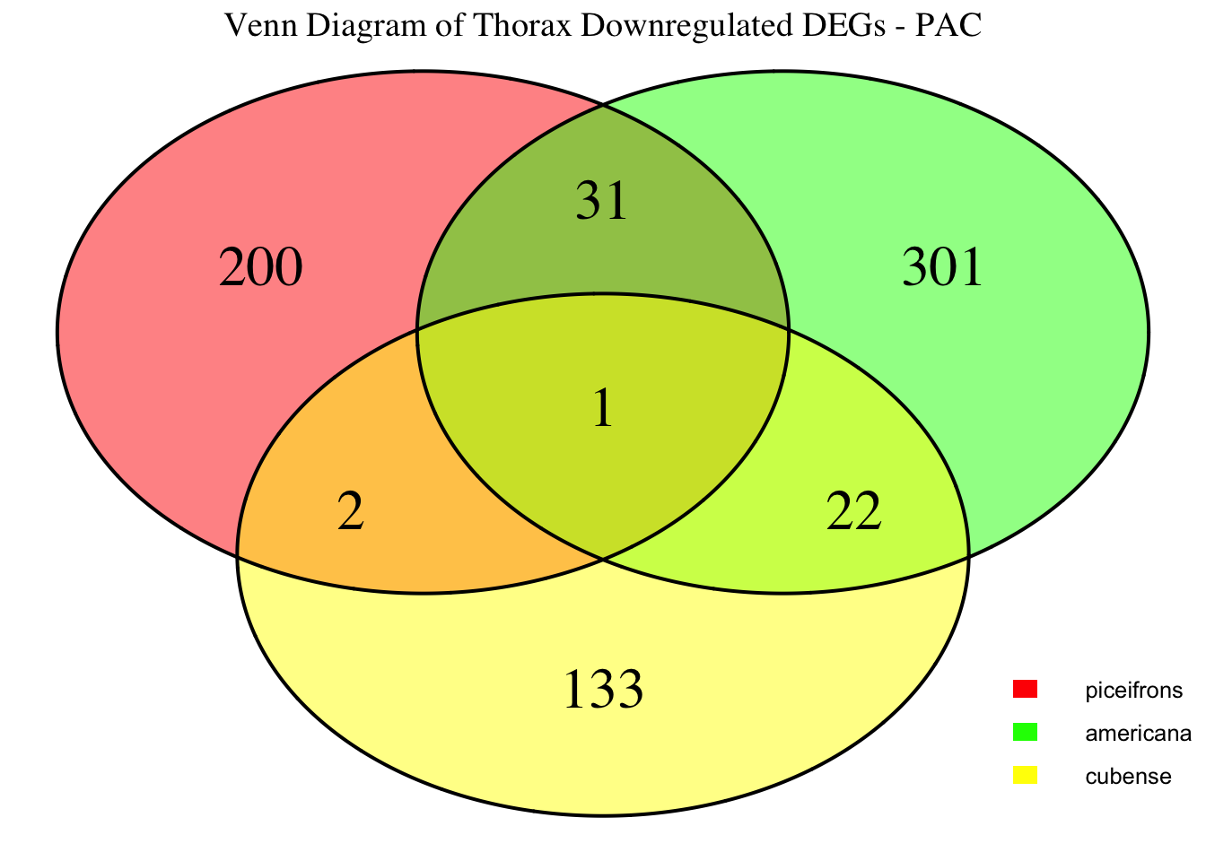
# Display the Venn diagram and datatable for all significant DEGs (PACclade)
display_venn_with_datatable(venn_data_all, "Venn Diagram of All Thorax DEGs - PAC", allspecies_df, filtered_final_orthotable)
Overlapping Orthogroups:
[1] "Unknown" "OG0000315" "OG0000142" "OG0001691" "OG0000111" "OG0000467"
[7] "OG0008500"
# Define the species for PACclade
PACclade <- c("piceifrons", "americana", "cubense")
input_file <- file.path(ortho_dir, "Results_I2/Orthogroups_genesproteinbiotype_Schistocerca_Jan2025.csv")
filtered_final_orthotable <- read.csv(input_file, header = TRUE, stringsAsFactors = FALSE)
# Initialize an empty list to store heatmap data for each species
heatmap_list <- list()

# Loop through each species to process their data
for (species in PACclade) {
  # Load DESeq2 results for head
  thorax_file <- file.path(workDir, "DEG_results/Bulk_RNAseq/", paste0(species, "/Thorax/DESeq2_results_Thorax_", species,".csv"))

  # Load the DESeq2 results
  thorax_data <- read.csv(thorax_file, stringsAsFactors = FALSE)

  # Check if data is empty and handle accordingly
  if (nrow(thorax_data) == 0) {
    message(paste("No data for species:", species))
    next  # Skip to the next species if there's no data
  }

  # Rename the "gene_id" column in filtered_final_orthotable for consistency
  colnames(filtered_final_orthotable)[colnames(filtered_final_orthotable) == "gene_id"] <- "GeneID"

  # Merge with filtered_final_orthotable to include Orthogroup
  merged_data <- merge(thorax_data, filtered_final_orthotable, by = "GeneID", all.x = TRUE)

  # Check if merge was successful
  if (nrow(merged_data) == 0) {
    message(paste("No matching data for species:", species))
    next  # Skip if no matching data after merging
  }

  # Filter for significant DEGs and select top 500 upregulated and downregulated genes for each tissue
  thorax_up <- merged_data %>%
    filter(padj < 0.05 & log2FoldChange > 1) %>%
    arrange(desc(log2FoldChange)) %>%
    slice(1:500)

  thorax_down <- merged_data %>%
    filter(padj < 0.05 & log2FoldChange < -1) %>%
    arrange(log2FoldChange) %>%
    slice(1:500)

  # Combine data and prepare for heatmap, adding the species column
  heatmap_data <- bind_rows(
    thorax_up %>% mutate(Tissue = "Thorax", Regulation = "Upregulated", Species = species),
    thorax_down %>% mutate(Tissue = "Thorax", Regulation = "Downregulated", Species = species)
  ) %>%
    select(Orthogroup, log2FoldChange, Tissue, Regulation, Species)

  # Append the heatmap data to the list
  heatmap_list[[species]] <- heatmap_data
}

# Combine all species data into a single dataframe for heatmap matrix preparation
final_heatmap_data <- bind_rows(heatmap_list)

# Check if final_heatmap_data is empty before proceeding
if (nrow(final_heatmap_data) == 0) {
    stop("No valid data available for heatmap generation.")
}

# Filter out rows with missing Orthogroup values
final_heatmap_data <- final_heatmap_data %>%
    filter(!is.na(Orthogroup))

# Check if there are any missing values in log2FoldChange (optional, just in case)
final_heatmap_data <- final_heatmap_data %>%
    filter(!is.na(log2FoldChange))

# Create heatmap matrix using Orthogroup instead of GeneID
heatmap_matrix <- final_heatmap_data %>%
    group_by(Orthogroup, Species) %>%
    summarize(
        Thorax_Combined = sum(log2FoldChange[Tissue == "Thorax"], na.rm = TRUE),
        .groups = 'drop'
    ) %>%
    pivot_wider(names_from = Species,
                values_from = Thorax_Combined,
                values_fill = list(Thorax_Combined = 0)) %>%
    column_to_rownames("Orthogroup") %>%
    as.matrix()

# Check if heatmap_matrix is empty
if (nrow(heatmap_matrix) == 0) {
    stop("No valid data available for heatmap matrix.")
}

# Define color palettes
# Define a custom color gradient where 0 is black
custom_color_palette1 <- colorRampPalette(c("cyan", "cyan3", "black", "orange3", "orange"))(100)

# Define a custom color gradient where 0 is white
custom_color_palette2 <- colorRampPalette(c("blue3", "blue", "white", "red", "red3"))(100)

# Define color breaks so that black is exactly at 0
max_abs_lfc <- max(abs(heatmap_matrix), na.rm = TRUE)  # Get max absolute log2FoldChange
color_breaks <- seq(-max_abs_lfc, max_abs_lfc, length.out = 100)  # Symmetric scale

# Create heatmap with clustering
pheatmap(
  heatmap_matrix,
  color = custom_color_palette2,
  breaks = color_breaks,
  cluster_rows = TRUE,  # Cluster genes
  cluster_cols = FALSE,  # Do not cluster species
  show_rownames = FALSE,
  show_colnames = TRUE,
  fontsize_row = 6,
  fontsize_col = 10,
  main = "Heatmap of Orthologs Expression in Thorax Tissue - STRATEGY 2"
)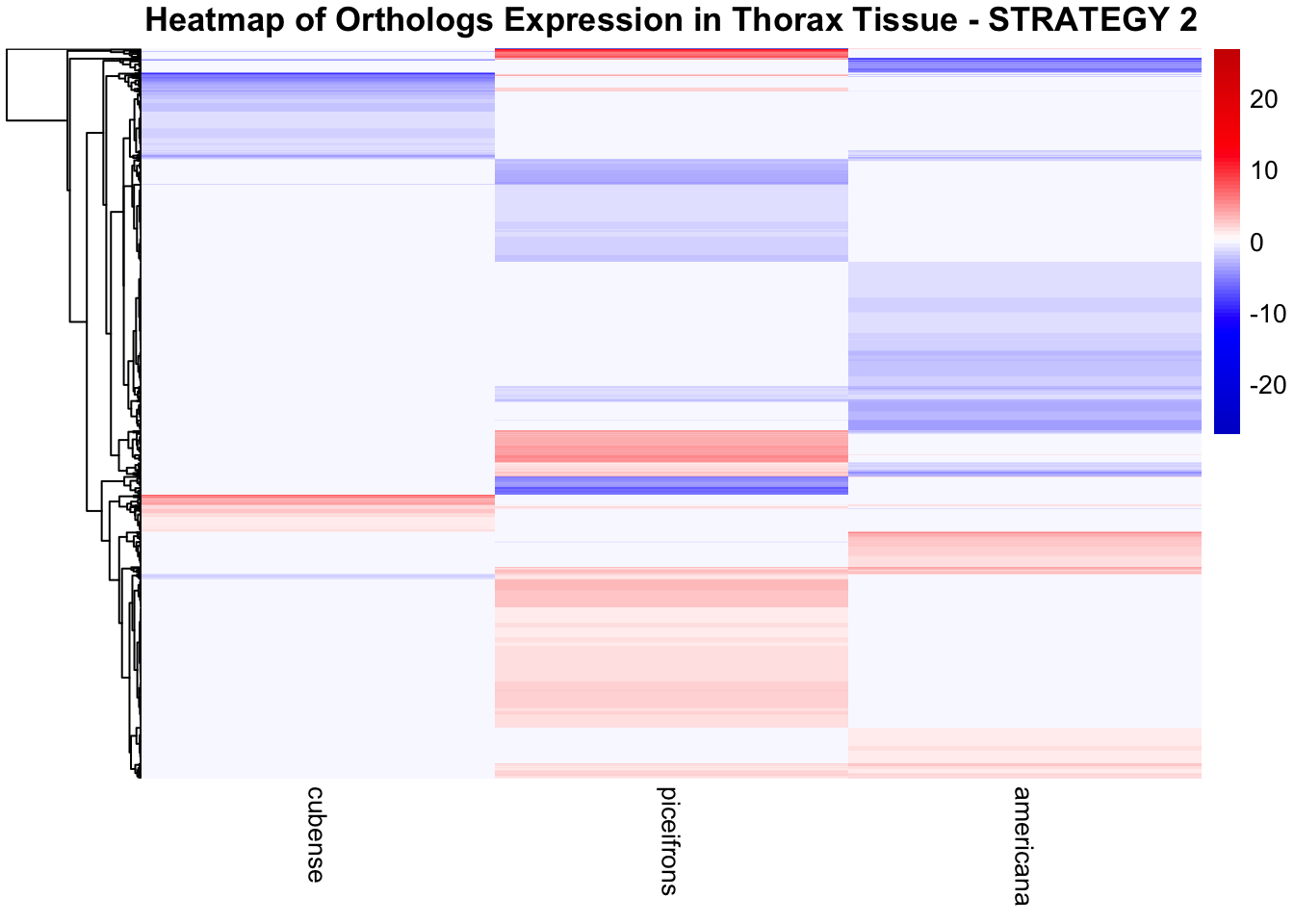
# Create heatmap without clustering columns
pheatmap(
  heatmap_matrix,
  color = custom_color_palette1,
  breaks = color_breaks,
  cluster_rows = TRUE,
  cluster_cols = FALSE,
  show_rownames = FALSE,
  show_colnames = TRUE,
  fontsize_row = 6,
  fontsize_col = 10,
  main = "Heatmap of Orthologs Expression in Thorax Tissue - STRATEGY 2"
)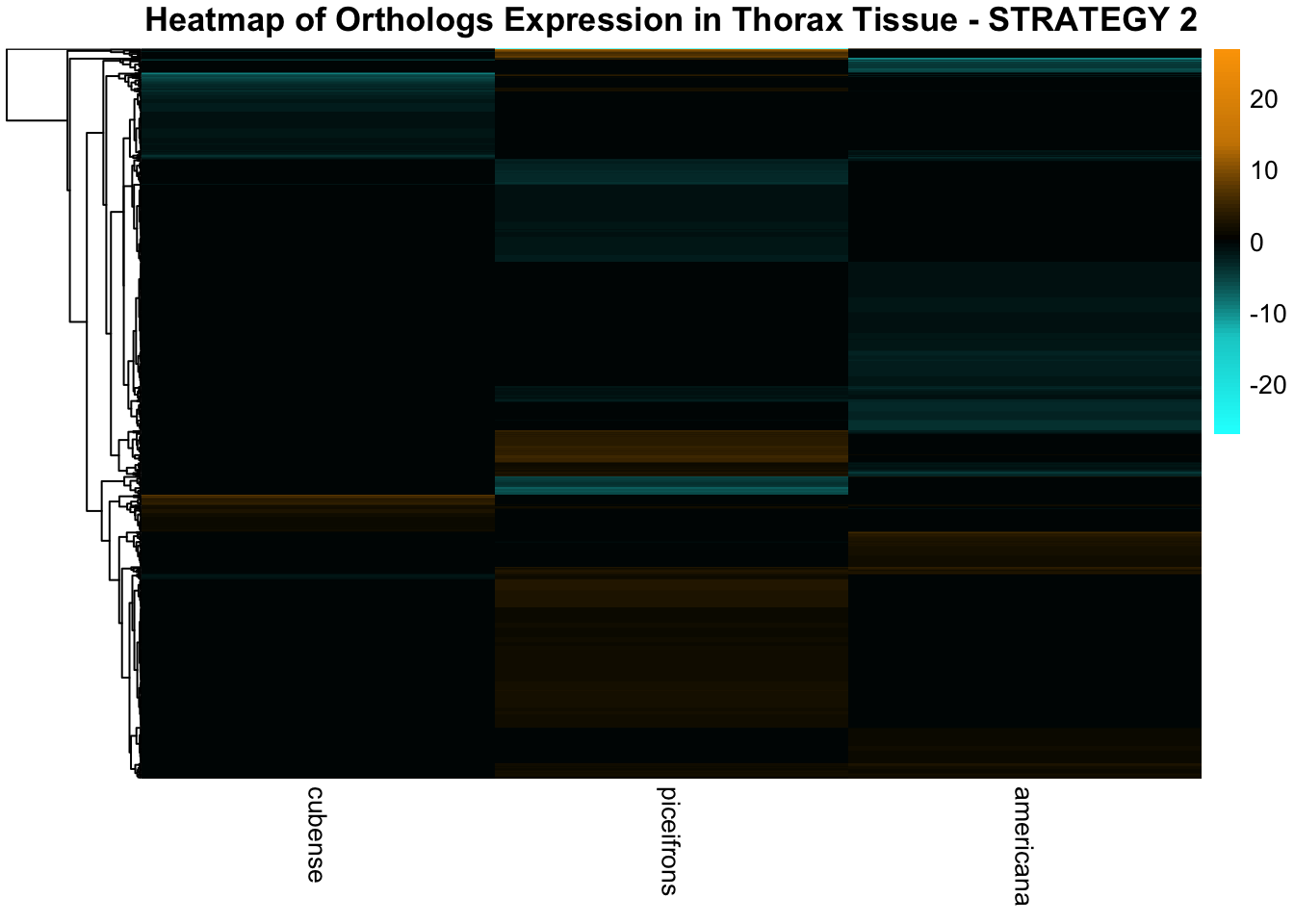
Plastic species
Head tissues
# Define the species for plastic_species
plastic_species <- c("gregaria", "piceifrons", "cancellata", "americana")
input_file <- file.path(ortho_dir, "Results_I2/Orthogroups_genesproteinbiotype_Schistocerca_Jan2025.csv")
filtered_final_orthotable <- read.csv(input_file, header = TRUE, stringsAsFactors = FALSE)


# Function to load DEGs for a given group of species
load_deg_data <- function(plastic_species, allspecies_df, filtered_final_orthotable) {
    degs_up <- list()
    degs_down <- list()
    degs_all <- list()

    # Rename the "gene_id" column in filtered_final_orthotable for consistency
    colnames(filtered_final_orthotable)[colnames(filtered_final_orthotable) == "gene_id"] <- "GeneID"

    for (species in plastic_species) {
        head_file <- file.path(workDir, "DEG_results/Bulk_RNAseq/", paste0(species, "/Head/DESeq2_results_Head_", species,".csv"))

        # Check if the file exists
        if (!file.exists(head_file)) {
            message(paste("File not found for species:", species))
            next  # Skip this iteration if the file is missing
        }

        # Read the data
        head_data <- read.csv(head_file, stringsAsFactors = FALSE)

        # Rename the "X" column to "GeneID"
        #colnames(head_data)[colnames(head_data) == "X"] <- "GeneID"

        # Merge DEG data with GeneType and Orthogroup information
        head_data_merged <- merge(head_data, allspecies_df[, c("GeneID", "GeneType", "Species")], by = "GeneID")
        head_data_merged <- merge(head_data_merged, filtered_final_orthotable[, c("GeneID", "Orthogroup")], by = "GeneID")

        # Handle missing Orthogroups
        head_data_merged$Orthogroup[is.na(head_data_merged$Orthogroup)] <- "Unknown"

        # Filter for significant DEGs (both upregulated and downregulated)
        head_up <- head_data_merged %>%
            filter(padj < 0.05 & log2FoldChange >= 1) %>%
            select(Orthogroup) %>%
            distinct()

        head_down <- head_data_merged %>%
            filter(padj < 0.05 & log2FoldChange <= -1) %>%
            select(Orthogroup) %>%
            distinct()

        all_deg <- head_data_merged %>%
            filter(padj < 0.05 & abs(log2FoldChange) >= 1) %>%
            select(Orthogroup) %>%
            distinct()

        # Store the DEGs in the list
        degs_up[[species]] <- head_up$Orthogroup
        degs_down[[species]] <- head_down$Orthogroup
        degs_all[[species]] <- all_deg$Orthogroup
    }

    return(list(up = degs_up, down = degs_down, all = degs_all))
}

# Function to display Venn diagram and corresponding datatable based on Orthogroups
# Function to display Venn diagram and corresponding datatable
display_venn_with_datatable <- function(venn_data, title, allspecies_df, filtered_final_orthotable) {

    # Calculate overlapping Orthogroups
    overlap_orthogroups <- Reduce(intersect, venn_data)

    # Print overlap info
    cat("Overlapping Orthogroups: \n")
    print(overlap_orthogroups)

    # If no overlaps exist, display a message and an empty plot
    if (length(overlap_orthogroups) == 0) {
        message("⚠️ No overlapping Orthogroups found. Displaying an empty Venn diagram.")

        # Create an empty Venn diagram placeholder
        plot.new()
        text(0.5, 0.5, "No overlapping Orthogroups found", cex = 1.5, col = "red")

        return(NULL)  # Exit the function gracefully
    }

    # Create a data frame for the overlapping Orthogroups
    overlap_df <- data.frame(Orthogroup = overlap_orthogroups)

    # Merge to get species and other information from filtered_final_orthotable
    meta_brock_df <- merge(overlap_df, filtered_final_orthotable, by = "Orthogroup", all.x = TRUE)

    # Ensure merged data exists
    if (nrow(meta_brock_df) == 0) {
        message("⚠️ Merge failed: No matching rows after merging Orthogroups.")
        return(NULL)
    }

    # Generate the Venn diagram
    venn_plot <- venn.diagram(
        x = venn_data,
        category.names = c("piceifrons", "americana", "cubense", "gregaria"),
        filename = NULL,
        output = TRUE,
        fill = c("red", "green", "yellow", "orange"),
        alpha = 0.5,
        cex = 2,
        cat.cex = 0,
        main = title,
        main.cex = 1.2
    )

    # Clear the current plotting area before drawing the Venn diagram
    grid.newpage()

    # Display the Venn diagram
    grid.draw(venn_plot)

    # Manually create a custom legend
    legend_labels <- c("piceifrons", "americana", "cubense", "gregaria")
    legend_colors <- c("red", "green", "yellow", "orange")

    # Positioning the legend lower on the right side of the plot
    legend_x <- unit(0.85, "npc")  # Adjust x position
    legend_y <- unit(0.2, "npc")   # Lower the legend vertically

    # Draw the legend
    for (i in 1:length(legend_labels)) {
        grid.rect(x = legend_x, y = legend_y - unit((i - 1) * 0.05, "npc"),
                  width = unit(0.02, "npc"), height = unit(0.02, "npc"),
                  gp = gpar(fill = legend_colors[i], col = NA))
        grid.text(label = legend_labels[i], x = legend_x + unit(0.05, "npc"),
                  y = legend_y - unit((i - 1) * 0.05, "npc"),
                  just = "left", gp = gpar(cex = 0.8))
    }

    # Display the merged overlapping Orthogroups table with datatable
    datatable(meta_brock_df, options = list(
        pageLength = 10,
        scrollX = TRUE,
        autoWidth = TRUE,
        searchHighlight = TRUE
    ),
    rownames = FALSE,
    escape = FALSE
    ) %>%
        formatStyle(
            'Species', target = 'cell',
            fontStyle = 'italic'
        ) %>%
        formatStyle(
            columns = names(meta_brock_df),
            target = 'row',
            color = styleEqual(c("red", "blue", "black"), c("red", "blue", "black")),
            fontWeight = styleEqual(c("bold", "normal"), c("bold", "normal")),
            backgroundColor = styleEqual(c("red", "blue", "black"), c("white", "white", "white"))
        )
}

# Example for testing with your data (for plastic_species)
venn_data_plastic_species <- load_deg_data(plastic_species, allspecies_df, filtered_final_orthotable)

# Prepare the data for the Venn diagrams for plastic_species
venn_data_up <- list(
  gregaria = venn_data_plastic_species$up[["gregaria"]],
  piceifrons = venn_data_plastic_species$up[["piceifrons"]],
  cancellata = venn_data_plastic_species$up[["cancellata"]],
  americana = venn_data_plastic_species$up[["americana"]]
)

venn_data_down <- list(
  gregaria = venn_data_plastic_species$down[["gregaria"]],
  piceifrons = venn_data_plastic_species$down[["piceifrons"]],
  cancellata = venn_data_plastic_species$down[["cancellata"]],
  americana = venn_data_plastic_species$down[["americana"]]
)

venn_data_all <- list(
  gregaria = venn_data_plastic_species$all[["gregaria"]],
  piceifrons = venn_data_plastic_species$all[["piceifrons"]],
  cancellata = venn_data_plastic_species$all[["cancellata"]],
  americana = venn_data_plastic_species$all[["americana"]]
)

# Display the Venn diagram and datatable for head upregulated DEGs (plastic_species)
display_venn_with_datatable(venn_data_up, "Venn Diagram of Head Upregulated DEGs - Plastic Species", allspecies_df, filtered_final_orthotable)
Overlapping Orthogroups:
[1] "Unknown" "OG0007485" "OG0004381" "OG0000630" "OG0010634" "OG0000447"
# Display the Venn diagram and datatable for head downregulated DEGs (plastic_species)
display_venn_with_datatable(venn_data_down, "Venn Diagram of Head Downregulated DEGs - Plastic Species", allspecies_df, filtered_final_orthotable)
Overlapping Orthogroups:
[1] "Unknown" "OG0008546" "OG0004570" "OG0009787" "OG0011171" "OG0003935"
[7] "OG0000505" "OG0000273" "OG0000149"
# Display the Venn diagram and datatable for all significant DEGs (plastic_species)
display_venn_with_datatable(venn_data_all, "Venn Diagram of All Head DEGs - Plastic Species", allspecies_df, filtered_final_orthotable)
Overlapping Orthogroups:
[1] "Unknown" "OG0007485" "OG0004381" "OG0000630" "OG0008546" "OG0004570"
[7] "OG0009787" "OG0010634" "OG0000447" "OG0011171" "OG0005490" "OG0003935"
[13] "OG0000505" "OG0000273" "OG0000149"
# Define the species for Group 1
plastic_species <- c("gregaria", "piceifrons", "cancellata", "americana")
input_file <- file.path(ortho_dir, "Results_I2/Orthogroups_genesproteinbiotype_Schistocerca_Jan2025.csv")
filtered_final_orthotable <- read.csv(input_file, header = TRUE, stringsAsFactors = FALSE)
# Initialize an empty list to store heatmap data for each species
heatmap_list <- list()

# Loop through each species to process their data
for (species in plastic_species) {
  # Load DESeq2 results for head
  head_file <- file.path(workDir, "DEG_results/Bulk_RNAseq/", paste0(species, "/Head/DESeq2_results_Head_", species,".csv"))

  # Load the DESeq2 results
  head_data <- read.csv(head_file, stringsAsFactors = FALSE)

  # Check if data is empty and handle accordingly
  if (nrow(head_data) == 0) {
    message(paste("No data for species:", species))
    next  # Skip to the next species if there's no data
  }

  # Rename the "gene_id" column in filtered_final_orthotable for consistency
  colnames(filtered_final_orthotable)[colnames(filtered_final_orthotable) == "gene_id"] <- "GeneID"

  # Merge with filtered_final_orthotable to include Orthogroup
  merged_data <- merge(head_data, filtered_final_orthotable, by = "GeneID", all.x = TRUE)

  # Check if merge was successful
  if (nrow(merged_data) == 0) {
    message(paste("No matching data for species:", species))
    next  # Skip if no matching data after merging
  }

  # Filter for significant DEGs and select top 500 upregulated and downregulated genes for each tissue
  head_up <- merged_data %>%
    filter(padj < 0.05 & log2FoldChange > 1) %>%
    arrange(desc(log2FoldChange)) %>%
    slice(1:500)

  head_down <- merged_data %>%
    filter(padj < 0.05 & log2FoldChange < -1) %>%
    arrange(log2FoldChange) %>%
    slice(1:500)

  # Combine data and prepare for heatmap, adding the species column
  heatmap_data <- bind_rows(
    head_up %>% mutate(Tissue = "Head", Regulation = "Upregulated", Species = species),
    head_down %>% mutate(Tissue = "Head", Regulation = "Downregulated", Species = species)
  ) %>%
    select(Orthogroup, log2FoldChange, Tissue, Regulation, Species)

  # Append the heatmap data to the list
  heatmap_list[[species]] <- heatmap_data
}

# Combine all species data into a single dataframe for heatmap matrix preparation
final_heatmap_data <- bind_rows(heatmap_list)

# Check if final_heatmap_data is empty before proceeding
if (nrow(final_heatmap_data) == 0) {
    stop("No valid data available for heatmap generation.")
}

# Filter out rows with missing Orthogroup values
final_heatmap_data <- final_heatmap_data %>%
    filter(!is.na(Orthogroup))

# Check if there are any missing values in log2FoldChange (optional, just in case)
final_heatmap_data <- final_heatmap_data %>%
    filter(!is.na(log2FoldChange))

# Create heatmap matrix using Orthogroup instead of GeneID
heatmap_matrix <- final_heatmap_data %>%
    group_by(Orthogroup, Species) %>%
    summarize(
        Head_Combined = sum(log2FoldChange[Tissue == "Head"], na.rm = TRUE),
        .groups = 'drop'
    ) %>%
    pivot_wider(names_from = Species,
                values_from = Head_Combined,
                values_fill = list(Head_Combined = 0)) %>%
    column_to_rownames("Orthogroup") %>%
    as.matrix()

# Check if heatmap_matrix is empty
if (nrow(heatmap_matrix) == 0) {
    stop("No valid data available for heatmap matrix.")
}

# Define color palettes
# Define a custom color gradient where 0 is black
custom_color_palette1 <- colorRampPalette(c("cyan", "cyan3", "black", "orange3", "orange"))(100)

# Define a custom color gradient where 0 is white
custom_color_palette2 <- colorRampPalette(c("blue3", "blue", "white", "red", "red3"))(100)

# Define color breaks so that black is exactly at 0
max_abs_lfc <- max(abs(heatmap_matrix), na.rm = TRUE)  # Get max absolute log2FoldChange
color_breaks <- seq(-max_abs_lfc, max_abs_lfc, length.out = 100)  # Symmetric scale

# Create heatmap with clustering
pheatmap(
  heatmap_matrix,
  color = custom_color_palette2,
  breaks = color_breaks,
  cluster_rows = TRUE,  # Cluster genes
  cluster_cols = FALSE,  # Do not cluster species
  show_rownames = FALSE,
  show_colnames = TRUE,
  fontsize_row = 6,
  fontsize_col = 10,
  main = "Heatmap of Orthologs Expression in Head Tissue - STRATEGY 2"
)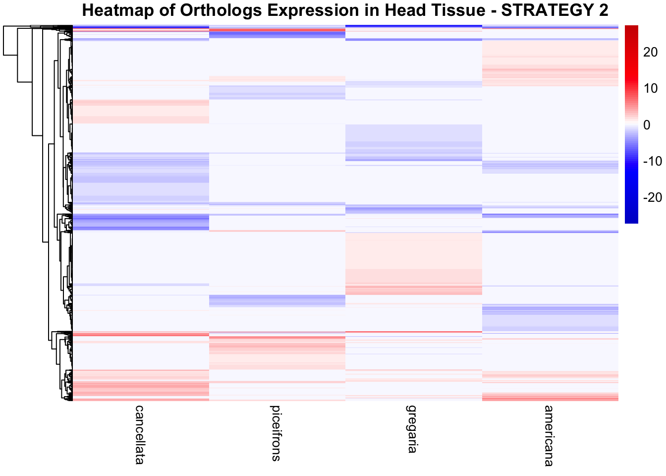
# Create heatmap without clustering columns
pheatmap(
  heatmap_matrix,
  color = custom_color_palette1,
  breaks = color_breaks,
  cluster_rows = TRUE,
  cluster_cols = FALSE,
  show_rownames = FALSE,
  show_colnames = TRUE,
  fontsize_row = 6,
  fontsize_col = 10,
  main = "Heatmap of Orthologs Expression in Head Tissue - STRATEGY 2"
)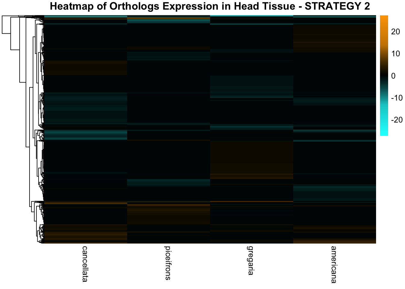
Thorax tissues
# Define the species for plastic_species
plastic_species <- c("gregaria", "piceifrons", "cancellata", "americana")
input_file <- file.path(ortho_dir, "Results_I2/Orthogroups_genesproteinbiotype_Schistocerca_Jan2025.csv")
filtered_final_orthotable <- read.csv(input_file, header = TRUE, stringsAsFactors = FALSE)


# Function to load DEGs for a given group of species
load_deg_data <- function(plastic_species, allspecies_df, filtered_final_orthotable) {
    degs_up <- list()
    degs_down <- list()
    degs_all <- list()

    # Rename the "gene_id" column in filtered_final_orthotable for consistency
    colnames(filtered_final_orthotable)[colnames(filtered_final_orthotable) == "gene_id"] <- "GeneID"

    for (species in plastic_species) {
        thorax_file <- file.path(workDir, "DEG_results/Bulk_RNAseq/", paste0(species, "/Thorax/DESeq2_results_Thorax_", species,".csv"))

        # Check if the file exists
        if (!file.exists(thorax_file)) {
            message(paste("File not found for species:", species))
            next  # Skip this iteration if the file is missing
        }

        # Read the data
        thorax_data <- read.csv(thorax_file, stringsAsFactors = FALSE)

        # Rename the "X" column to "GeneID"
        #colnames(thorax_data)[colnames(thorax_data) == "X"] <- "GeneID"

        # Merge DEG data with GeneType and Orthogroup information
        thorax_data_merged <- merge(thorax_data, allspecies_df[, c("GeneID", "GeneType", "Species")], by = "GeneID")
        thorax_data_merged <- merge(thorax_data_merged, filtered_final_orthotable[, c("GeneID", "Orthogroup")], by = "GeneID")

        # Handle missing Orthogroups
        thorax_data_merged$Orthogroup[is.na(thorax_data_merged$Orthogroup)] <- "Unknown"

        # Filter for significant DEGs (both upregulated and downregulated)
        thorax_up <- thorax_data_merged %>%
            filter(padj < 0.05 & log2FoldChange >= 1) %>%
            select(Orthogroup) %>%
            distinct()

        thorax_down <- thorax_data_merged %>%
            filter(padj < 0.05 & log2FoldChange <= -1) %>%
            select(Orthogroup) %>%
            distinct()

        all_deg <- thorax_data_merged %>%
            filter(padj < 0.05 & abs(log2FoldChange) >= 1) %>%
            select(Orthogroup) %>%
            distinct()

        # Store the DEGs in the list
        degs_up[[species]] <- thorax_up$Orthogroup
        degs_down[[species]] <- thorax_down$Orthogroup
        degs_all[[species]] <- all_deg$Orthogroup
    }

    return(list(up = degs_up, down = degs_down, all = degs_all))
}

# Function to display Venn diagram and corresponding datatable based on Orthogroups
# Function to display Venn diagram and corresponding datatable
display_venn_with_datatable <- function(venn_data, title, allspecies_df, filtered_final_orthotable) {

    # Calculate overlapping Orthogroups
    overlap_orthogroups <- Reduce(intersect, venn_data)

    # Print overlap info
    cat("Overlapping Orthogroups: \n")
    print(overlap_orthogroups)

    # If no overlaps exist, display a message and an empty plot
    if (length(overlap_orthogroups) == 0) {
        message("⚠️ No overlapping Orthogroups found. Displaying an empty Venn diagram.")

        # Create an empty Venn diagram placeholder
        plot.new()
        text(0.5, 0.5, "No overlapping Orthogroups found", cex = 1.5, col = "red")

        return(NULL)  # Exit the function gracefully
    }

    # Create a data frame for the overlapping Orthogroups
    overlap_df <- data.frame(Orthogroup = overlap_orthogroups)

    # Merge to get species and other information from filtered_final_orthotable
    meta_brock_df <- merge(overlap_df, filtered_final_orthotable, by = "Orthogroup", all.x = TRUE)

    # Ensure merged data exists
    if (nrow(meta_brock_df) == 0) {
        message("⚠️ Merge failed: No matching rows after merging Orthogroups.")
        return(NULL)
    }

    # Generate the Venn diagram
    venn_plot <- venn.diagram(
        x = venn_data,
        category.names = c("piceifrons", "americana", "cubense", "gregaria"),
        filename = NULL,
        output = TRUE,
        fill = c("red", "green", "yellow", "orange"),
        alpha = 0.5,
        cex = 2,
        cat.cex = 0,
        main = title,
        main.cex = 1.2
    )

    # Clear the current plotting area before drawing the Venn diagram
    grid.newpage()

    # Display the Venn diagram
    grid.draw(venn_plot)

    # Manually create a custom legend
    legend_labels <- c("piceifrons", "americana", "cubense", "gregaria")
    legend_colors <- c("red", "green", "yellow", "orange")

    # Positioning the legend lower on the right side of the plot
    legend_x <- unit(0.85, "npc")  # Adjust x position
    legend_y <- unit(0.2, "npc")   # Lower the legend vertically

    # Draw the legend
    for (i in 1:length(legend_labels)) {
        grid.rect(x = legend_x, y = legend_y - unit((i - 1) * 0.05, "npc"),
                  width = unit(0.02, "npc"), height = unit(0.02, "npc"),
                  gp = gpar(fill = legend_colors[i], col = NA))
        grid.text(label = legend_labels[i], x = legend_x + unit(0.05, "npc"),
                  y = legend_y - unit((i - 1) * 0.05, "npc"),
                  just = "left", gp = gpar(cex = 0.8))
    }

    # Display the merged overlapping Orthogroups table with datatable
    datatable(meta_brock_df, options = list(
        pageLength = 10,
        scrollX = TRUE,
        autoWidth = TRUE,
        searchHighlight = TRUE
    ),
    rownames = FALSE,
    escape = FALSE
    ) %>%
        formatStyle(
            'Species', target = 'cell',
            fontStyle = 'italic'
        ) %>%
        formatStyle(
            columns = names(meta_brock_df),
            target = 'row',
            color = styleEqual(c("red", "blue", "black"), c("red", "blue", "black")),
            fontWeight = styleEqual(c("bold", "normal"), c("bold", "normal")),
            backgroundColor = styleEqual(c("red", "blue", "black"), c("white", "white", "white"))
        )
}

# Example for testing with your data (for plastic_species)
venn_data_plastic_species <- load_deg_data(plastic_species, allspecies_df, filtered_final_orthotable)

# Prepare the data for the Venn diagrams for plastic_species
venn_data_up <- list(
  gregaria = venn_data_plastic_species$up[["gregaria"]],
  piceifrons = venn_data_plastic_species$up[["piceifrons"]],
  cancellata = venn_data_plastic_species$up[["cancellata"]],
  americana = venn_data_plastic_species$up[["americana"]]
)

venn_data_down <- list(
  gregaria = venn_data_plastic_species$down[["gregaria"]],
  piceifrons = venn_data_plastic_species$down[["piceifrons"]],
  cancellata = venn_data_plastic_species$down[["cancellata"]],
  americana = venn_data_plastic_species$down[["americana"]]
)

venn_data_all <- list(
  gregaria = venn_data_plastic_species$all[["gregaria"]],
  piceifrons = venn_data_plastic_species$all[["piceifrons"]],
  cancellata = venn_data_plastic_species$all[["cancellata"]],
  americana = venn_data_plastic_species$all[["americana"]]
)

# Display the Venn diagram and datatable for thorax upregulated DEGs (plastic_species)
display_venn_with_datatable(venn_data_up, "Venn Diagram of Thorax Upregulated DEGs - Plastic Species", allspecies_df, filtered_final_orthotable)
Overlapping Orthogroups:
[1] "Unknown" "OG0012855" "OG0004381" "OG0008773" "OG0013891" "OG0002449"
[7] "OG0000196" "OG0010743" "OG0011869" "OG0006295" "OG0006293" "OG0005991"
[13] "OG0003684" "OG0003702" "OG0003704" "OG0006530" "OG0006498" "OG0007438"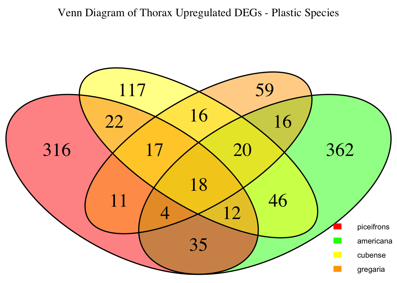
# Display the Venn diagram and datatable for head downregulated DEGs (plastic_species)
display_venn_with_datatable(venn_data_down, "Venn Diagram of Thorax Downregulated DEGs - Plastic Species", allspecies_df, filtered_final_orthotable)
Overlapping Orthogroups:
[1] "Unknown" "OG0008629" "OG0009787" "OG0010410" "OG0011346" "OG0000270"
[7] "OG0003407" "OG0000008" "OG0000505"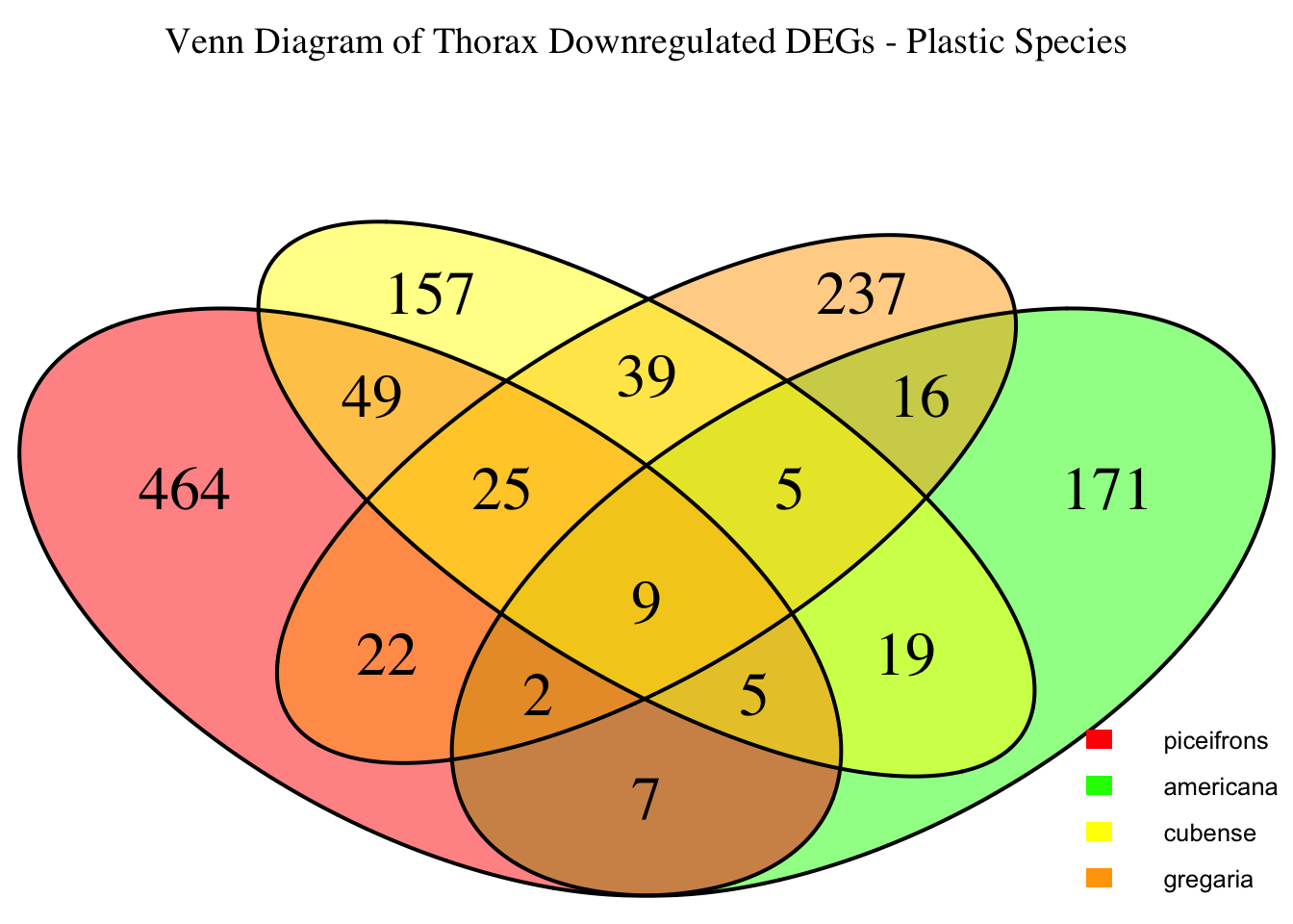
# Display the Venn diagram and datatable for all significant DEGs (plastic_species)
display_venn_with_datatable(venn_data_all, "Venn Diagram of All Thorax DEGs - Plastic Species", allspecies_df, filtered_final_orthotable)
Overlapping Orthogroups:
[1] "Unknown" "OG0012855" "OG0004381" "OG0012943" "OG0008773" "OG0013891"
[7] "OG0008629" "OG0002449" "OG0000196" "OG0009787" "OG0010410" "OG0010743"
[13] "OG0011346" "OG0011869" "OG0000396" "OG0000270" "OG0003407" "OG0006295"
[19] "OG0006293" "OG0000008" "OG0005991" "OG0003684" "OG0003702" "OG0003704"
[25] "OG0006530" "OG0006498" "OG0000505" "OG0000504" "OG0000037" "OG0007438"
# Define the species for PACclade
plastic_species <- c("gregaria", "piceifrons", "cancellata", "americana")
input_file <- file.path(ortho_dir, "Results_I2/Orthogroups_genesproteinbiotype_Schistocerca_Jan2025.csv")
filtered_final_orthotable <- read.csv(input_file, header = TRUE, stringsAsFactors = FALSE)
# Initialize an empty list to store heatmap data for each species
heatmap_list <- list()

# Loop through each species to process their data
for (species in plastic_species) {
  # Load DESeq2 results for head
  thorax_file <- file.path(workDir, "DEG_results/Bulk_RNAseq/", paste0(species, "/Thorax/DESeq2_results_Thorax_", species,".csv"))

  # Load the DESeq2 results
  thorax_data <- read.csv(thorax_file, stringsAsFactors = FALSE)

  # Check if data is empty and handle accordingly
  if (nrow(thorax_data) == 0) {
    message(paste("No data for species:", species))
    next  # Skip to the next species if there's no data
  }

  # Rename the "gene_id" column in filtered_final_orthotable for consistency
  #colnames(filtered_final_orthotable)[colnames(filtered_final_orthotable) == "gene_id"] <- "GeneID"

  # Merge with filtered_final_orthotable to include Orthogroup
  merged_data <- merge(thorax_data, filtered_final_orthotable, by = "GeneID", all.x = TRUE)

  # Check if merge was successful
  if (nrow(merged_data) == 0) {
    message(paste("No matching data for species:", species))
    next  # Skip if no matching data after merging
  }

  # Filter for significant DEGs and select top 500 upregulated and downregulated genes for each tissue
  thorax_up <- merged_data %>%
    filter(padj < 0.05 & log2FoldChange > 1) %>%
    arrange(desc(log2FoldChange)) %>%
    slice(1:500)

  thorax_down <- merged_data %>%
    filter(padj < 0.05 & log2FoldChange < -1) %>%
    arrange(log2FoldChange) %>%
    slice(1:500)

  # Combine data and prepare for heatmap, adding the species column
  heatmap_data <- bind_rows(
    thorax_up %>% mutate(Tissue = "Thorax", Regulation = "Upregulated", Species = species),
    thorax_down %>% mutate(Tissue = "Thorax", Regulation = "Downregulated", Species = species)
  ) %>%
    select(Orthogroup, log2FoldChange, Tissue, Regulation, Species)

  # Append the heatmap data to the list
  heatmap_list[[species]] <- heatmap_data
}

# Combine all species data into a single dataframe for heatmap matrix preparation
final_heatmap_data <- bind_rows(heatmap_list)

# Check if final_heatmap_data is empty before proceeding
if (nrow(final_heatmap_data) == 0) {
    stop("No valid data available for heatmap generation.")
}

# Filter out rows with missing Orthogroup values
final_heatmap_data <- final_heatmap_data %>%
    filter(!is.na(Orthogroup))

# Check if there are any missing values in log2FoldChange (optional, just in case)
final_heatmap_data <- final_heatmap_data %>%
    filter(!is.na(log2FoldChange))

# Create heatmap matrix using Orthogroup instead of GeneID
heatmap_matrix <- final_heatmap_data %>%
    group_by(Orthogroup, Species) %>%
    summarize(
        Thorax_Combined = sum(log2FoldChange[Tissue == "Thorax"], na.rm = TRUE),
        .groups = 'drop'
    ) %>%
    pivot_wider(names_from = Species,
                values_from = Thorax_Combined,
                values_fill = list(Thorax_Combined = 0)) %>%
    column_to_rownames("Orthogroup") %>%
    as.matrix()

# Check if heatmap_matrix is empty
if (nrow(heatmap_matrix) == 0) {
    stop("No valid data available for heatmap matrix.")
}

# Define color palettes
# Define a custom color gradient where 0 is black
custom_color_palette1 <- colorRampPalette(c("cyan", "cyan3", "black", "orange3", "orange"))(100)

# Define a custom color gradient where 0 is white
custom_color_palette2 <- colorRampPalette(c("blue3", "blue", "white", "red", "red3"))(100)

# Define color breaks so that black is exactly at 0
max_abs_lfc <- max(abs(heatmap_matrix), na.rm = TRUE)  # Get max absolute log2FoldChange
color_breaks <- seq(-max_abs_lfc, max_abs_lfc, length.out = 100)  # Symmetric scale

# Create heatmap with clustering
pheatmap(
  heatmap_matrix,
  color = custom_color_palette2,
  breaks = color_breaks,
  cluster_rows = TRUE,  # Cluster genes
  cluster_cols = FALSE,  # Do not cluster species
  show_rownames = FALSE,
  show_colnames = TRUE,
  fontsize_row = 6,
  fontsize_col = 10,
  main = "Heatmap of Orthologs Expression in Thorax Tissue - STRATEGY 2"
)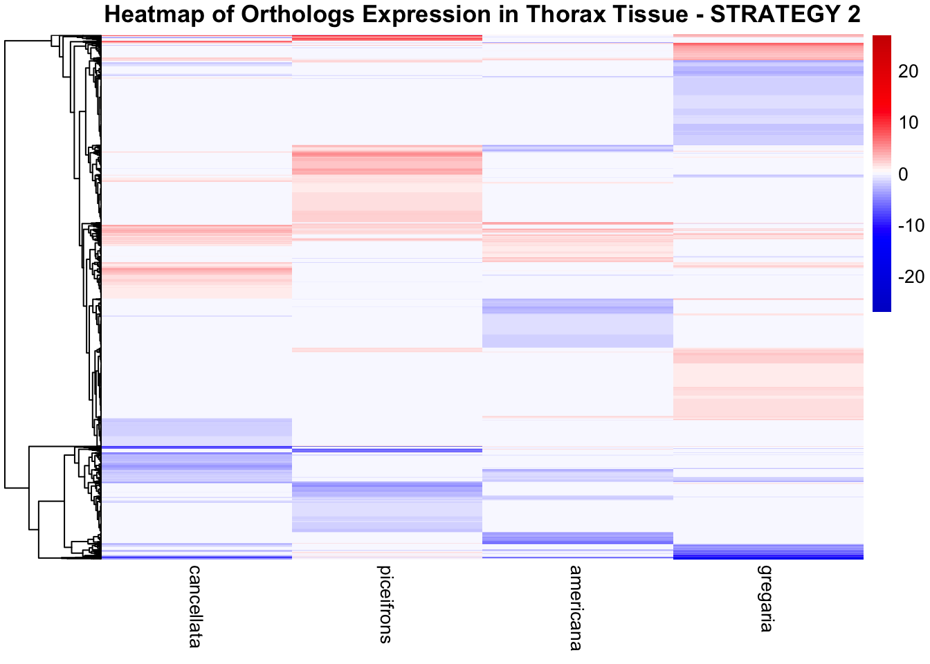
# Create heatmap without clustering columns
pheatmap(
  heatmap_matrix,
  color = custom_color_palette1,
  breaks = color_breaks,
  cluster_rows = TRUE,
  cluster_cols = FALSE,
  show_rownames = FALSE,
  show_colnames = TRUE,
  fontsize_row = 6,
  fontsize_col = 10,
  main = "Heatmap of Orthologs Expression in Thorax Tissue - STRATEGY 2"
)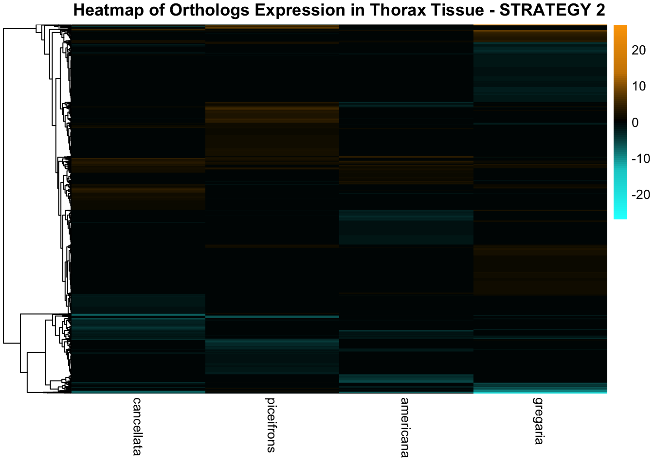
Five species
Combined tissues
# Load orthogroup mapping
input_file <- file.path(ortho_dir, "Results_I2/Orthogroups_genesproteinbiotype_Schistocerca_Jan2025.csv")
filtered_final_orthotable <- read.csv(input_file, header = TRUE, stringsAsFactors = FALSE)

# Ensure column names are correctly set
if ("gene_id" %in% colnames(filtered_final_orthotable)) {
  colnames(filtered_final_orthotable)[colnames(filtered_final_orthotable) == "gene_id"] <- "GeneID"
}

# Select only relevant columns and ensure uniqueness
filtered_final_orthotable <- filtered_final_orthotable %>%
  select(GeneID, Orthogroup) %>%
  distinct(GeneID, .keep_all = TRUE)  # Ensure one entry per GeneID

# Define species list
allspecies <- c("gregaria", "piceifrons", "cancellata", "americana", "cubense")

# Function to load DEGs for a given set of species and a specific tissue
load_deg_data <- function(species_list, tissue) {
  degs_up <- list()
  degs_down <- list()
  degs_all <- list()

  for (species in species_list) {
    # Define the correct file path based on tissue
    deg_file <- file.path(workDir, "DEG_results/Bulk_RNAseq/", paste0(species, "/", tissue, "/DESeq2_results_", tissue, "_", species, ".csv"))
    # Read DESeq2 results
    deg_data <- read.csv(deg_file, stringsAsFactors = FALSE)

    # Ensure 'GeneID' column exists (some DESeq2 outputs use 'X')
    #if (!"GeneID" %in% colnames(deg_data)) {
    #  if ("X" %in% colnames(deg_data)) {
    #    colnames(deg_data)[colnames(deg_data) == "X"] <- "GeneID"
    #  } else {
    #    message(paste("No GeneID column found for", species, "in", tissue, "- Skipping"))
    #    next
    #  }
    #}

    # Convert to character for safe merging
    deg_data$GeneID <- as.character(deg_data$GeneID)
    filtered_final_orthotable$GeneID <- as.character(filtered_final_orthotable$GeneID)

    # Merge with orthogroup information
    deg_data <- left_join(deg_data, filtered_final_orthotable, by = "GeneID") %>%
      mutate(Orthogroup = ifelse(is.na(Orthogroup), "Unassigned", Orthogroup))  # Handle missing orthogroups

    # Check if data is empty
    if (nrow(deg_data) == 0) {
      message(paste("No data for species:", species, "in tissue:", tissue))
      next
    }

    # Filter for significant DEGs based on `log2FoldChange`
    upregulated <- deg_data %>%
      filter(padj < 0.05 & log2FoldChange >= 1) %>%
      select(Orthogroup) %>%
      distinct()

    downregulated <- deg_data %>%
      filter(padj < 0.05 & log2FoldChange <= -1) %>%
      select(Orthogroup) %>%
      distinct()

    all_degs <- deg_data %>%
      filter(padj < 0.05 & abs(log2FoldChange) >= 1) %>%
      select(Orthogroup) %>%
      distinct()

    # Store the DEGs in the lists
    degs_up[[species]] <- upregulated$Orthogroup
    degs_down[[species]] <- downregulated$Orthogroup
    degs_all[[species]] <- all_degs$Orthogroup
  }

  return(list(up = degs_up, down = degs_down, all = degs_all))
}

# Load DEG data for Head
venn_data_allspecies_head <- load_deg_data(allspecies, "Head")

# Load DEG data for Thorax
venn_data_allspecies_thorax <- load_deg_data(allspecies, "Thorax")

# Function to generate Venn diagrams with Orthogroups
display_venn_with_datatable <- function(venn_data, title) {
  # Calculate overlapping genes
  overlap_orthogroups <- Reduce(intersect, venn_data)

  # Create a dataframe for overlapping orthogroups
  overlap_df <- data.frame(Orthogroup = overlap_orthogroups)

  # Generate the Venn diagram
  venn_plot <- venn.diagram(
    x = venn_data,
    category.names = allspecies,
    filename = NULL,
    output = TRUE,
    fill = c("orange", "red", "orchid", "green", "yellow"),
    alpha = 0.5,
    cex = 2,
    cat.cex = 0,
    main = title,
    main.cex = 1.2
  )

  # Clear plotting area and display Venn diagram
  grid.newpage()
  grid.draw(venn_plot)

  # Manually create a custom legend
  legend_labels <- allspecies
  legend_colors <- c("orange", "red", "orchid", "green", "yellow")

  # Position legend
  legend_x <- unit(0.85, "npc")
  legend_y <- unit(0.2, "npc")

  for (i in 1:length(legend_labels)) {
    grid.rect(x = legend_x, y = legend_y - unit((i - 1) * 0.05, "npc"),
              width = unit(0.02, "npc"), height = unit(0.02, "npc"),
              gp = gpar(fill = legend_colors[i], col = NA))
    grid.text(label = legend_labels[i], x = legend_x + unit(0.05, "npc"),
              y = legend_y - unit((i - 1) * 0.05, "npc"),
              just = "left", gp = gpar(cex = 0.8))
  }

  # Display the overlapping Orthogroups as a datatable
  datatable(overlap_df, options = list(
      pageLength = 10,
      scrollX = TRUE,
      autoWidth = TRUE,
      searchHighlight = TRUE
  ),
  rownames = FALSE)
}

# Display Venn diagrams and tables for HEAD
display_venn_with_datatable(venn_data_allspecies_head$up, "Venn Diagram of Upregulated Orthogroups - Head")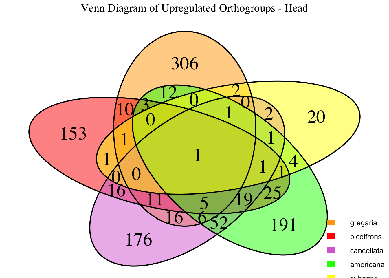
| Version | Author | Date |
|---|---|---|
| b540a1e | Maeva TECHER | 2025-02-27 |
display_venn_with_datatable(venn_data_allspecies_head$down, "Venn Diagram of Downregulated Orthogroups - Head")
| Version | Author | Date |
|---|---|---|
| b540a1e | Maeva TECHER | 2025-02-27 |
display_venn_with_datatable(venn_data_allspecies_head$all, "Venn Diagram of All Significant Orthogroups - Head")
| Version | Author | Date |
|---|---|---|
| b540a1e | Maeva TECHER | 2025-02-27 |
# Display Venn diagrams and tables for THORAX
display_venn_with_datatable(venn_data_allspecies_thorax$up, "Venn Diagram of Upregulated Orthogroups - Thorax")
| Version | Author | Date |
|---|---|---|
| b540a1e | Maeva TECHER | 2025-02-27 |
display_venn_with_datatable(venn_data_allspecies_thorax$down, "Venn Diagram of Downregulated Orthogroups - Thorax")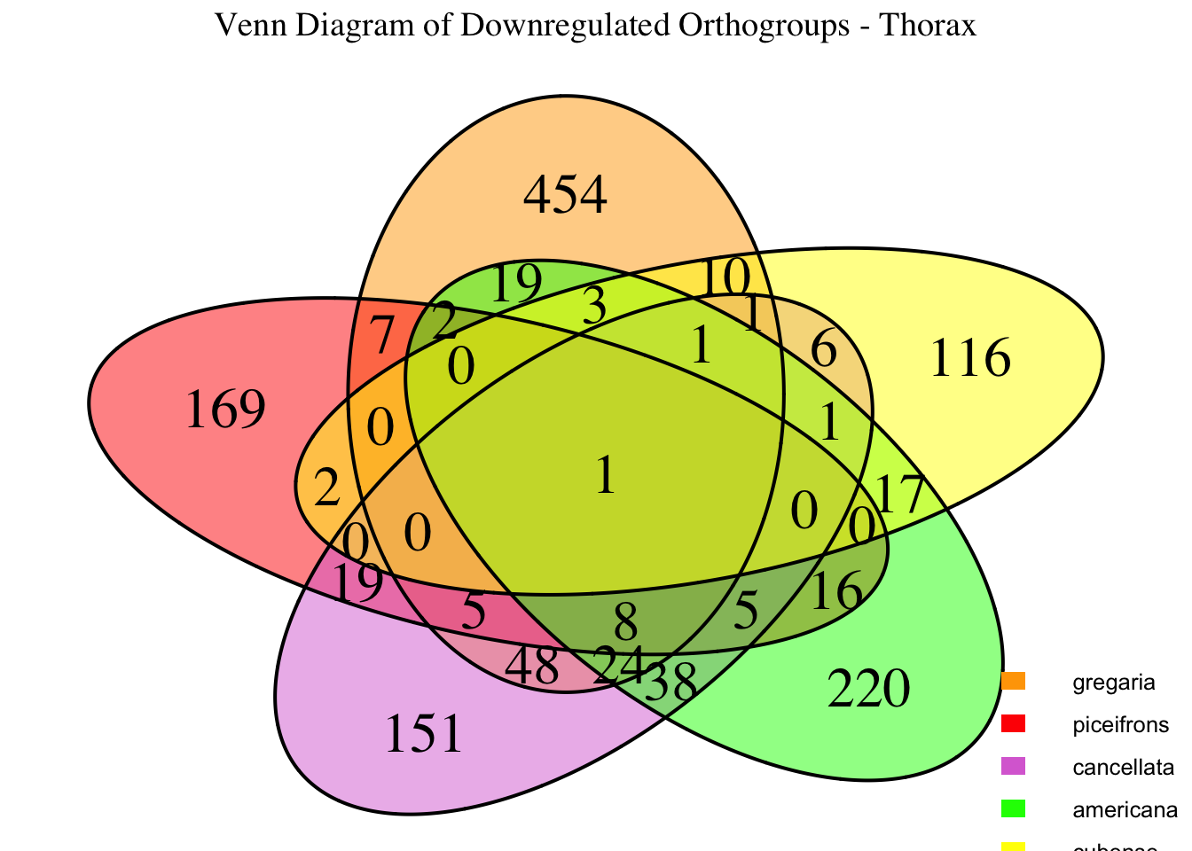
| Version | Author | Date |
|---|---|---|
| b540a1e | Maeva TECHER | 2025-02-27 |
display_venn_with_datatable(venn_data_allspecies_thorax$all, "Venn Diagram of All Significant Orthogroups - Thorax")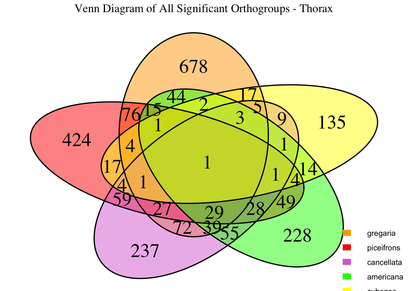
| Version | Author | Date |
|---|---|---|
| b540a1e | Maeva TECHER | 2025-02-27 |
# Load Orthogroup information
input_file <- file.path(ortho_dir, "Results_I2/Orthogroups_genesproteinbiotype_Schistocerca_Jan2025.csv")
filtered_final_orthotable <- read.csv(input_file, header = TRUE, stringsAsFactors = FALSE)

# Ensure correct column names
if ("gene_id" %in% colnames(filtered_final_orthotable)) {
  colnames(filtered_final_orthotable)[colnames(filtered_final_orthotable) == "gene_id"] <- "GeneID"
}

# Select relevant columns and ensure uniqueness
filtered_final_orthotable <- filtered_final_orthotable %>%
  select(GeneID, Orthogroup) %>%
  distinct(GeneID, .keep_all = TRUE)  # Keep unique mapping

# Define species order explicitly
species_order <- c("nitens", "cubense", "americana", "piceifrons", "cancellata", "gregaria")

# Initialize an empty list to store heatmap data
heatmap_list <- list()

# Loop through each species to process their data
for (species in species_order) {
  message(paste("Processing species:", species))

  # Define file paths
  head_file <- file.path(workDir, "DEG_results/Bulk_RNAseq/", paste0(species, "/Head/DESeq2_results_Head_", species,".csv"))
  thorax_file <- file.path(workDir, "DEG_results/Bulk_RNAseq/", paste0(species, "/Thorax/DESeq2_results_Thorax_", species,".csv"))

  # Check if files exist before loading
  if (!file.exists(head_file)) {
    message(paste("Missing Head file for:", species, "- Assigning empty dataset"))
    head_data <- data.frame(GeneID = character(), padj = numeric(), log2FoldChange = numeric(), stringsAsFactors = FALSE)
  } else {
    head_data <- tryCatch(read.csv(head_file, stringsAsFactors = FALSE), error = function(e) data.frame())
  }

  if (!file.exists(thorax_file)) {
    message(paste("Missing Thorax file for:", species, "- Assigning empty dataset"))
    thorax_data <- data.frame(GeneID = character(), padj = numeric(), log2FoldChange = numeric(), stringsAsFactors = FALSE)
  } else {
    thorax_data <- tryCatch(read.csv(thorax_file, stringsAsFactors = FALSE), error = function(e) data.frame())
  }

  # Ensure GeneID column exists
  #if (!"GeneID" %in% colnames(head_data) && "X" %in% colnames(head_data)) {
  #  colnames(head_data)[colnames(head_data) == "X"] <- "GeneID"
  #}
  #if (!"GeneID" %in% colnames(thorax_data) && "X" %in% colnames(thorax_data)) {
  #  colnames(thorax_data)[colnames(thorax_data) == "X"] <- "GeneID"
  #}

  # Convert GeneID to character
  head_data$GeneID <- as.character(head_data$GeneID)
  thorax_data$GeneID <- as.character(thorax_data$GeneID)
  filtered_final_orthotable$GeneID <- as.character(filtered_final_orthotable$GeneID)

  # Ensure species is not skipped if one dataset is empty
  if (nrow(head_data) == 0 && nrow(thorax_data) == 0) {
    message(paste("No data for species:", species, "- Skipping"))
    next
  }

  # If thorax data is missing, assign zero values
  if (nrow(thorax_data) == 0) {
    message(paste("No Thorax data for:", species, "- Assigning 0 values"))
    thorax_data <- data.frame(GeneID = head_data$GeneID, padj = 1, log2FoldChange = 0, stringsAsFactors = FALSE)
  }

  # Merge with orthogroup information
  head_data <- left_join(head_data, filtered_final_orthotable, by = "GeneID") %>%
    mutate(Orthogroup = ifelse(is.na(Orthogroup), "Unassigned", Orthogroup))

  thorax_data <- left_join(thorax_data, filtered_final_orthotable, by = "GeneID") %>%
    mutate(Orthogroup = ifelse(is.na(Orthogroup), "Unassigned", Orthogroup))

  # Filter for significant DEGs and select top 500 upregulated and downregulated genes per tissue
  head_up <- head_data %>%
    filter(padj < 0.05 & log2FoldChange > 1) %>%
    arrange(desc(log2FoldChange)) %>%
    slice(1:500)

  head_down <- head_data %>%
    filter(padj < 0.05 & log2FoldChange < -1) %>%
    arrange(log2FoldChange) %>%
    slice(1:500)

  thorax_up <- thorax_data %>%
    filter(padj < 0.05 & log2FoldChange > 1) %>%
    arrange(desc(log2FoldChange)) %>%
    slice(1:500)

  thorax_down <- thorax_data %>%
    filter(padj < 0.05 & log2FoldChange < -1) %>%
    arrange(log2FoldChange) %>%
    slice(1:500)

  # Combine data and prepare for heatmap
  heatmap_data <- bind_rows(
    head_up %>% mutate(Tissue = "Head", Regulation = "Upregulated", Species = species),
    head_down %>% mutate(Tissue = "Head", Regulation = "Downregulated", Species = species),
    thorax_up %>% mutate(Tissue = "Thorax", Regulation = "Upregulated", Species = species),
    thorax_down %>% mutate(Tissue = "Thorax", Regulation = "Downregulated", Species = species)
  ) %>%
    select(Orthogroup, log2FoldChange, Tissue, Regulation, Species)

  # Append to heatmap list
  heatmap_list[[species]] <- heatmap_data
}

# Combine all species data
final_heatmap_data <- bind_rows(heatmap_list)

# Ensure species order in the data
final_heatmap_data$Species <- factor(final_heatmap_data$Species, levels = species_order)

# Create heatmap matrix (Thorax only)
heatmap_matrix <- final_heatmap_data %>%
    group_by(Orthogroup, Species) %>%  # Remove Tissue to ensure unique Orthogroup rows
    summarize(log2FoldChange = mean(log2FoldChange, na.rm = TRUE), .groups = "drop") %>%
    pivot_wider(names_from = Species, values_from = log2FoldChange, values_fill = 0) %>%
    distinct(Orthogroup, .keep_all = TRUE) %>%  # Ensure unique Orthogroup rows
    column_to_rownames("Orthogroup") %>%
    as.matrix()

# Explicitly reorder the columns in heatmap_matrix
heatmap_matrix <- heatmap_matrix[, species_order, drop = FALSE]  # Ensure order is applied

# Define color palettes
custom_cyan_orange_palette <- colorRampPalette(c("cyan", "cyan2", "cyan3", "black", "orange3", "orange2", "orange"))(100)
custom_blue_red_palette <- colorRampPalette(c("blue3", "blue2", "blue1", "white", "red", "red2", "red3"))(100)

# Define color breaks
max_abs_lfc <- max(abs(heatmap_matrix), na.rm = TRUE)
color_breaks <- seq(-max_abs_lfc, max_abs_lfc, length.out = 100)

# Generate heatmaps
pheatmap(
  heatmap_matrix,
  color = custom_blue_red_palette,
  breaks = color_breaks,
  cluster_rows = TRUE,
  cluster_cols = FALSE,
  show_rownames = FALSE,
  show_colnames = TRUE,
  fontsize_row = 6,
  fontsize_col = 10,
  main = "Heatmap of Orthologs Expression in Head and Thorax Tissue - STRATEGY 2"
)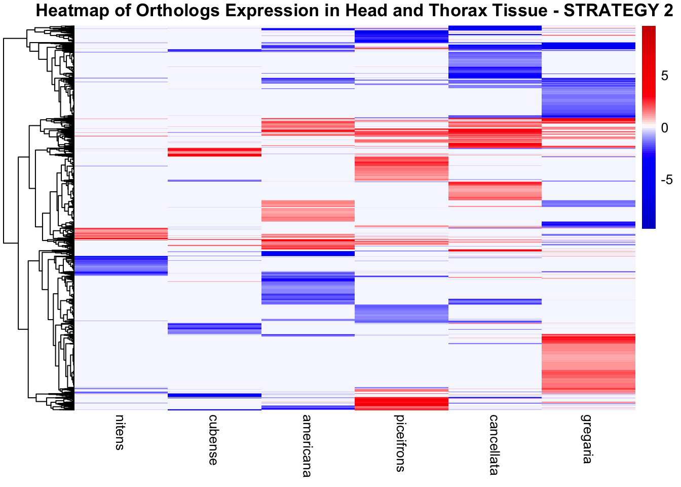
| Version | Author | Date |
|---|---|---|
| b540a1e | Maeva TECHER | 2025-02-27 |
pheatmap(
  heatmap_matrix,
  color = custom_cyan_orange_palette,
  breaks = color_breaks,
  cluster_rows = TRUE,
  cluster_cols = FALSE,
  show_rownames = FALSE,
  show_colnames = TRUE,
  fontsize_row = 6,
  fontsize_col = 10,
  main = "Heatmap of Orthologs Expression in Head and Thorax Tissue- STRATEGY 2"
)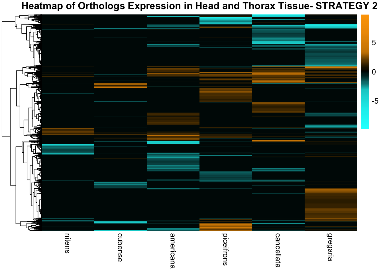
| Version | Author | Date |
|---|---|---|
| b540a1e | Maeva TECHER | 2025-02-27 |
Head tissues
# Load orthogroup mapping
input_file <- file.path(ortho_dir, "Results_I2/Orthogroups_genesproteinbiotype_Schistocerca_Jan2025.csv")
filtered_final_orthotable <- read.csv(input_file, header = TRUE, stringsAsFactors = FALSE)

# Ensure column names are correctly set
if ("gene_id" %in% colnames(filtered_final_orthotable)) {
  colnames(filtered_final_orthotable)[colnames(filtered_final_orthotable) == "gene_id"] <- "GeneID"
}

# Select only relevant columns and ensure uniqueness
filtered_final_orthotable <- filtered_final_orthotable %>%
  select(GeneID, Orthogroup) %>%
  distinct(GeneID, .keep_all = TRUE)  # Ensure one entry per GeneID

# Define species list
allspecies <- c("gregaria", "piceifrons", "cancellata", "americana", "cubense")

# Function to load DEGs for a given set of species and a specific tissue (ONLY HEAD)
load_deg_data <- function(species_list) {
  degs_up <- list()
  degs_down <- list()
  degs_all <- list()

  for (species in species_list) {
    # Define the correct file path for Head
        deg_file <- file.path(workDir, "DEG_results/Bulk_RNAseq/", paste0(species, "/Head/DESeq2_results_Head_", species, ".csv"))

    # Read DESeq2 results
    deg_data <- read.csv(deg_file, stringsAsFactors = FALSE)

    # Ensure 'GeneID' column exists (some DESeq2 outputs use 'X')
    #if (!"GeneID" %in% colnames(deg_data)) {
    #  if ("X" %in% colnames(deg_data)) {
    #    colnames(deg_data)[colnames(deg_data) == "X"] <- "GeneID"
    #  } else {
    #    message(paste("No GeneID column found for", species, "in Head - Skipping"))
    #    next
    #  }
    #}

    # Convert to character for safe merging
    deg_data$GeneID <- as.character(deg_data$GeneID)
    filtered_final_orthotable$GeneID <- as.character(filtered_final_orthotable$GeneID)

    # Merge with orthogroup information
    deg_data <- left_join(deg_data, filtered_final_orthotable, by = "GeneID") %>%
      mutate(Orthogroup = ifelse(is.na(Orthogroup), "Unassigned", Orthogroup))  # Handle missing orthogroups

    # Check if data is empty
    if (nrow(deg_data) == 0) {
      message(paste("No data for species:", species, "in Head"))
      next
    }

    # Filter for significant DEGs based on `log2FoldChange`
    upregulated <- deg_data %>%
      filter(padj < 0.05 & log2FoldChange >= 1) %>%
      select(Orthogroup) %>%
      distinct()

    downregulated <- deg_data %>%
      filter(padj < 0.05 & log2FoldChange <= -1) %>%
      select(Orthogroup) %>%
      distinct()

    all_degs <- deg_data %>%
      filter(padj < 0.05 & abs(log2FoldChange) >= 1) %>%
      select(Orthogroup) %>%
      distinct()

    # Store the DEGs in the lists
    degs_up[[species]] <- upregulated$Orthogroup
    degs_down[[species]] <- downregulated$Orthogroup
    degs_all[[species]] <- all_degs$Orthogroup
  }

  return(list(up = degs_up, down = degs_down, all = degs_all))
}

# Load DEG data for Head only
venn_data_allspecies_head <- load_deg_data(allspecies)

# Function to generate Venn diagrams with Orthogroups (ONLY HEAD)
display_venn_with_datatable <- function(venn_data, title) {
  # Calculate overlapping genes
  overlap_orthogroups <- Reduce(intersect, venn_data)

  # Create a dataframe for overlapping orthogroups
  overlap_df <- data.frame(Orthogroup = overlap_orthogroups)

  # Generate the Venn diagram
  venn_plot <- venn.diagram(
    x = venn_data,
    category.names = allspecies,
    filename = NULL,
    output = TRUE,
    fill = c("orange", "red", "orchid", "green", "yellow"),
    alpha = 0.5,
    cex = 2,
    cat.cex = 0,
    main = title,
    main.cex = 1.2
  )

  # Clear plotting area and display Venn diagram
  grid.newpage()
  grid.draw(venn_plot)

  # Display overlapping Orthogroups as a datatable
  datatable(overlap_df, options = list(
      pageLength = 10,
      scrollX = TRUE,
      autoWidth = TRUE,
      searchHighlight = TRUE
  ), rownames = FALSE)
}

# Display Venn diagrams and tables for HEAD only
display_venn_with_datatable(venn_data_allspecies_head$up, "Venn Diagram of Upregulated Orthogroups - Head")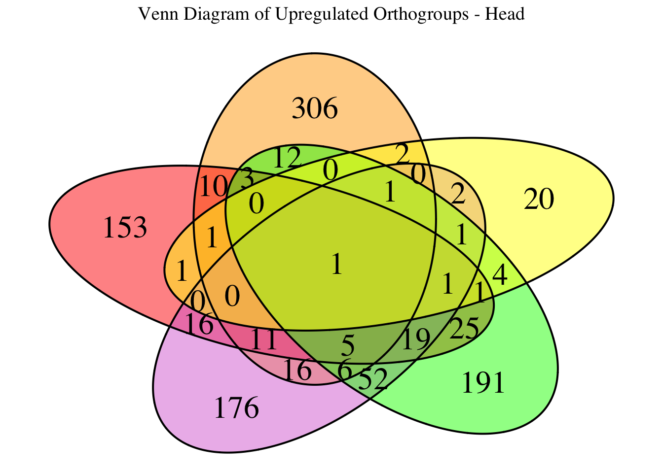
| Version | Author | Date |
|---|---|---|
| b540a1e | Maeva TECHER | 2025-02-27 |
display_venn_with_datatable(venn_data_allspecies_head$down, "Venn Diagram of Downregulated Orthogroups - Head")
| Version | Author | Date |
|---|---|---|
| b540a1e | Maeva TECHER | 2025-02-27 |
display_venn_with_datatable(venn_data_allspecies_head$all, "Venn Diagram of All Significant Orthogroups - Head")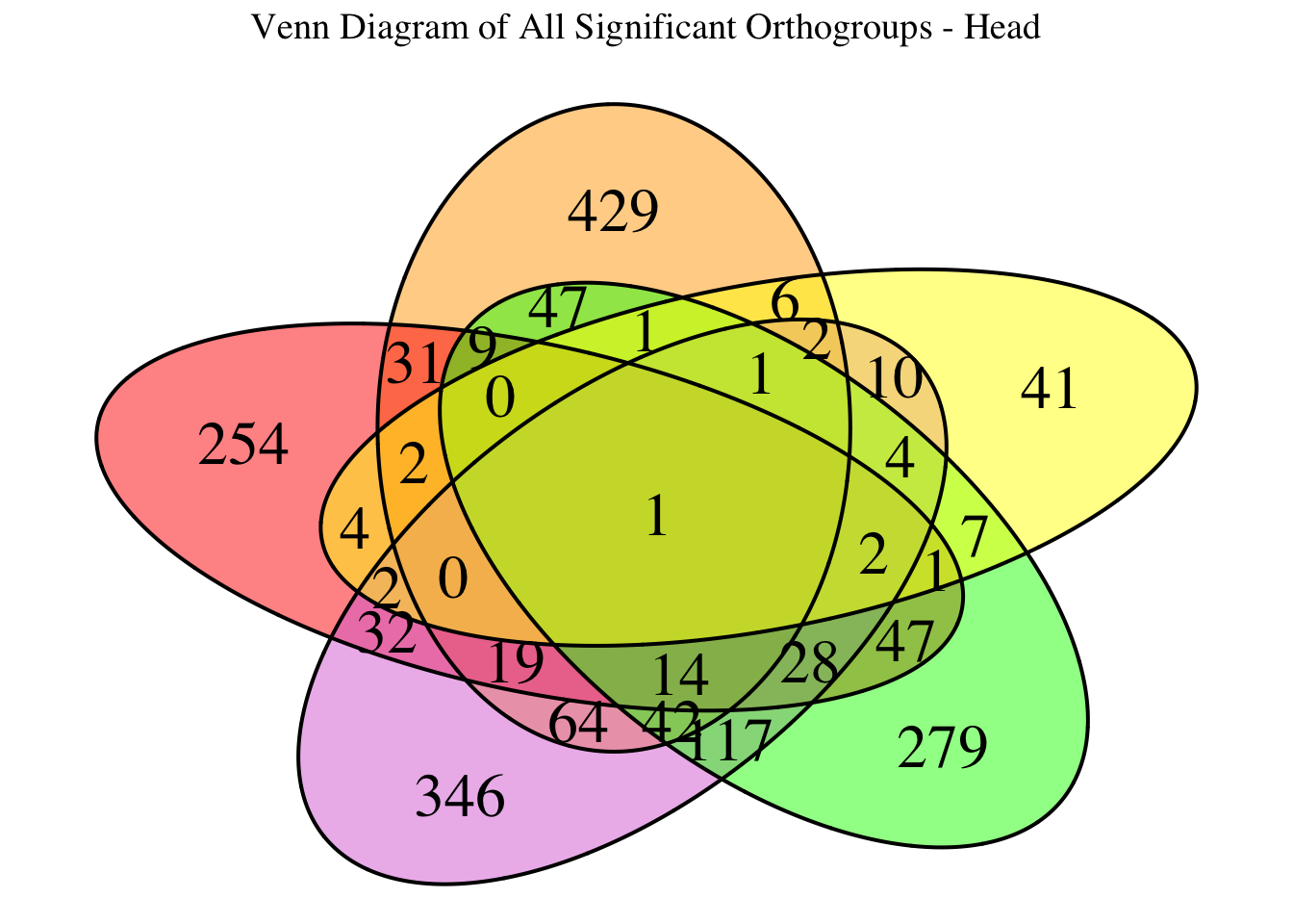
| Version | Author | Date |
|---|---|---|
| b540a1e | Maeva TECHER | 2025-02-27 |
# Load Orthogroup information
input_file <- file.path(ortho_dir, "Results_I2/Orthogroups_genesproteinbiotype_Schistocerca_Jan2025.csv")
filtered_final_orthotable <- read.csv(input_file, header = TRUE, stringsAsFactors = FALSE)

# Ensure correct column names
if ("gene_id" %in% colnames(filtered_final_orthotable)) {
  colnames(filtered_final_orthotable)[colnames(filtered_final_orthotable) == "gene_id"] <- "GeneID"
}

# Select relevant columns and ensure uniqueness
filtered_final_orthotable <- filtered_final_orthotable %>%
  select(GeneID, Orthogroup) %>%
  distinct(GeneID, .keep_all = TRUE)  # Keep unique mapping

# Define species order explicitly
species_order <- c("nitens", "cubense", "americana", "piceifrons", "cancellata", "gregaria")

# Initialize an empty list to store heatmap data
heatmap_list <- list()

# Loop through each species to process their Head data
for (species in species_order) {
  message(paste("Processing species:", species))

  # Define file path for Head
  head_file <- file.path(workDir, "DEG_results/Bulk_RNAseq/", paste0(species, "/Head/DESeq2_results_Head_", species,".csv"))

  # Check if file exists before loading
  if (!file.exists(head_file)) {
    message(paste("Missing Head file for:", species, "- Assigning empty dataset"))
    head_data <- data.frame(GeneID = character(), padj = numeric(), log2FoldChange = numeric(), stringsAsFactors = FALSE)
  } else {
    head_data <- tryCatch(read.csv(head_file, stringsAsFactors = FALSE), error = function(e) data.frame())
  }

  # Ensure GeneID column exists
  #if (!"GeneID" %in% colnames(head_data) && "X" %in% colnames(head_data)) {
  #  colnames(head_data)[colnames(head_data) == "X"] <- "GeneID"
  #}

  # Convert GeneID to character
  head_data$GeneID <- as.character(head_data$GeneID)
  filtered_final_orthotable$GeneID <- as.character(filtered_final_orthotable$GeneID)

  # Merge with orthogroup information
  head_data <- left_join(head_data, filtered_final_orthotable, by = "GeneID") %>%
    mutate(Orthogroup = ifelse(is.na(Orthogroup), "Unassigned", Orthogroup))

  # Filter for significant DEGs and select top 500 upregulated and downregulated genes
  head_up <- head_data %>%
    filter(padj < 0.05 & log2FoldChange > 1) %>%
    arrange(desc(log2FoldChange)) %>%
    slice(1:500)

  head_down <- head_data %>%
    filter(padj < 0.05 & log2FoldChange < -1) %>%
    arrange(log2FoldChange) %>%
    slice(1:500)

  # Combine data and prepare for heatmap
  heatmap_data <- bind_rows(
    head_up %>% mutate(Tissue = "Head", Regulation = "Upregulated", Species = species),
    head_down %>% mutate(Tissue = "Head", Regulation = "Downregulated", Species = species)
  ) %>%
    select(Orthogroup, log2FoldChange, Tissue, Regulation, Species)

  # Append to heatmap list
  heatmap_list[[species]] <- heatmap_data
}

# Combine all species data
final_heatmap_data <- bind_rows(heatmap_list)

# Ensure all species are represented, even if they have no significant DEGs
for (species in species_order) {
    if (!species %in% unique(final_heatmap_data$Species)) {
        message(paste("Adding placeholder for missing species:", species))
        final_heatmap_data <- bind_rows(
            final_heatmap_data,
            data.frame(
                Orthogroup = "Unassigned",  # Placeholder Orthogroup
                log2FoldChange = 0,
                Tissue = "Head",
                Regulation = "None",
                Species = species
            )
        )
    }
}

# Ensure species order in the data
final_heatmap_data$Species <- factor(final_heatmap_data$Species, levels = species_order)

# Create heatmap matrix (Thorax only)
heatmap_matrix <- final_heatmap_data %>%
  group_by(Orthogroup, Species) %>%
  summarize(log2FoldChange = mean(log2FoldChange, na.rm = TRUE), .groups = "drop") %>%
  pivot_wider(names_from = Species, values_from = log2FoldChange, values_fill = 0) %>%
  column_to_rownames("Orthogroup") %>%
  as.matrix()

# Explicitly reorder the columns in heatmap_matrix
heatmap_matrix <- heatmap_matrix[, species_order, drop = FALSE]  # Ensure order is applied

# Define color palettes
custom_cyan_orange_palette <- colorRampPalette(c("cyan", "cyan2", "cyan3", "black", "orange3", "orange2", "orange"))(100)
custom_blue_red_palette <- colorRampPalette(c("blue3", "blue2", "blue1", "white", "red", "red2", "red3"))(100)

# Define color breaks
max_abs_lfc <- max(abs(heatmap_matrix), na.rm = TRUE)
color_breaks <- seq(-max_abs_lfc, max_abs_lfc, length.out = 100)

# Generate heatmaps (Only Head)
pheatmap(
  heatmap_matrix,
  color = custom_blue_red_palette,
  breaks = color_breaks,
  cluster_rows = TRUE,
  cluster_cols = FALSE,
  show_rownames = FALSE,
  show_colnames = TRUE,
  fontsize_row = 6,
  fontsize_col = 10,
  main = "Heatmap of Orthologs Expression in Head Tissue - STRATEGY 2"
)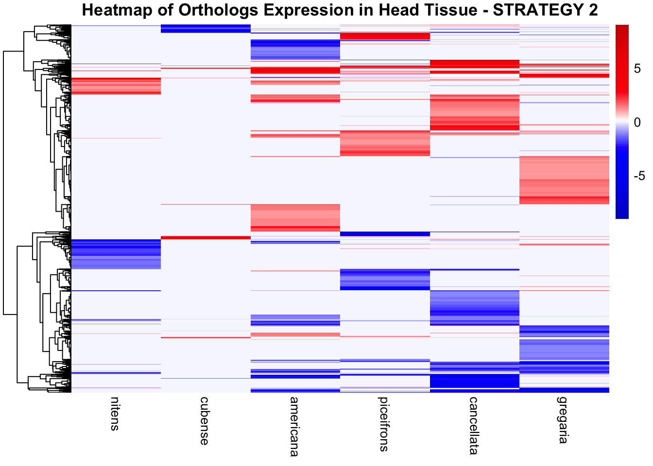
| Version | Author | Date |
|---|---|---|
| b540a1e | Maeva TECHER | 2025-02-27 |
pheatmap(
  heatmap_matrix,
  color = custom_cyan_orange_palette,
  breaks = color_breaks,
  cluster_rows = TRUE,
  cluster_cols = FALSE,
  show_rownames = FALSE,
  show_colnames = TRUE,
  fontsize_row = 6,
  fontsize_col = 10,
  main = "Heatmap of Orthologs Expression in Head Tissue - STRATEGY 2"
)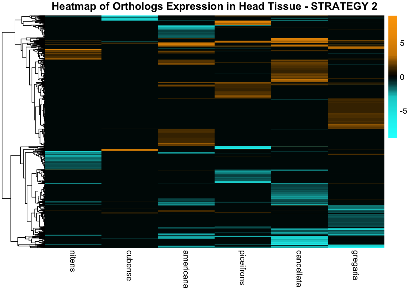
| Version | Author | Date |
|---|---|---|
| b540a1e | Maeva TECHER | 2025-02-27 |
Thorax tissues
# Load orthogroup mapping
input_file <- file.path(ortho_dir, "Results_I2/Orthogroups_genesproteinbiotype_Schistocerca_Jan2025.csv")
filtered_final_orthotable <- read.csv(input_file, header = TRUE, stringsAsFactors = FALSE)

# Ensure column names are correctly set
if ("gene_id" %in% colnames(filtered_final_orthotable)) {
  colnames(filtered_final_orthotable)[colnames(filtered_final_orthotable) == "gene_id"] <- "GeneID"
}

# Select only relevant columns and ensure uniqueness
filtered_final_orthotable <- filtered_final_orthotable %>%
  select(GeneID, Orthogroup) %>%
  distinct(GeneID, .keep_all = TRUE)  # Ensure one entry per GeneID

# Define species list
allspecies <- c("gregaria", "piceifrons", "cancellata", "americana", "cubense")

# Function to load DEGs for a given set of species and a specific tissue (ONLY thorax)
load_deg_data <- function(species_list) {
  degs_up <- list()
  degs_down <- list()
  degs_all <- list()

  for (species in species_list) {
    # Define the correct file path for thorax
    deg_file <- file.path(workDir, "DEG_results/Bulk_RNAseq/", paste0(species, "/Thorax/DESeq2_results_Thorax_", species, ".csv"))

    # Read DESeq2 results
    deg_data <- read.csv(deg_file, stringsAsFactors = FALSE)

    # Ensure 'GeneID' column exists (some DESeq2 outputs use 'X')
    #if (!"GeneID" %in% colnames(deg_data)) {
    #  if ("X" %in% colnames(deg_data)) {
    #    colnames(deg_data)[colnames(deg_data) == "X"] <- "GeneID"
    #  } else {
    #    message(paste("No GeneID column found for", species, "in Thorax - Skipping"))
    #    next
    #  }
    #}

    # Convert to character for safe merging
    deg_data$GeneID <- as.character(deg_data$GeneID)
    filtered_final_orthotable$GeneID <- as.character(filtered_final_orthotable$GeneID)

    # Merge with orthogroup information
    deg_data <- left_join(deg_data, filtered_final_orthotable, by = "GeneID") %>%
      mutate(Orthogroup = ifelse(is.na(Orthogroup), "Unassigned", Orthogroup))  # Handle missing orthogroups

    # Check if data is empty
    if (nrow(deg_data) == 0) {
      message(paste("No data for species:", species, "in Thorax"))
      next
    }

    # Filter for significant DEGs based on `log2FoldChange`
    upregulated <- deg_data %>%
      filter(padj < 0.05 & log2FoldChange >= 1) %>%
      select(Orthogroup) %>%
      distinct()

    downregulated <- deg_data %>%
      filter(padj < 0.05 & log2FoldChange <= -1) %>%
      select(Orthogroup) %>%
      distinct()

    all_degs <- deg_data %>%
      filter(padj < 0.05 & abs(log2FoldChange) >= 1) %>%
      select(Orthogroup) %>%
      distinct()

    # Store the DEGs in the lists
    degs_up[[species]] <- upregulated$Orthogroup
    degs_down[[species]] <- downregulated$Orthogroup
    degs_all[[species]] <- all_degs$Orthogroup
  }

  return(list(up = degs_up, down = degs_down, all = degs_all))
}

# Load DEG data for Thorax only
venn_data_allspecies_thorax <- load_deg_data(allspecies)

# Function to generate Venn diagrams with Orthogroups (ONLY thorax)
display_venn_with_datatable <- function(venn_data, title) {
  # Calculate overlapping genes
  overlap_orthogroups <- Reduce(intersect, venn_data)

  # Create a dataframe for overlapping orthogroups
  overlap_df <- data.frame(Orthogroup = overlap_orthogroups)

  # Generate the Venn diagram
  venn_plot <- venn.diagram(
    x = venn_data,
    category.names = allspecies,
    filename = NULL,
    output = TRUE,
    fill = c("orange", "red", "orchid", "green", "yellow"),
    alpha = 0.5,
    cex = 2,
    cat.cex = 0,
    main = title,
    main.cex = 1.2
  )

  # Clear plotting area and display Venn diagram
  grid.newpage()
  grid.draw(venn_plot)

  # Display overlapping Orthogroups as a datatable
  datatable(overlap_df, options = list(
      pageLength = 10,
      scrollX = TRUE,
      autoWidth = TRUE,
      searchHighlight = TRUE
  ), rownames = FALSE)
}

# Display Venn diagrams and tables for thorax only
display_venn_with_datatable(venn_data_allspecies_thorax$up, "Venn Diagram of Upregulated Orthogroups - Thorax")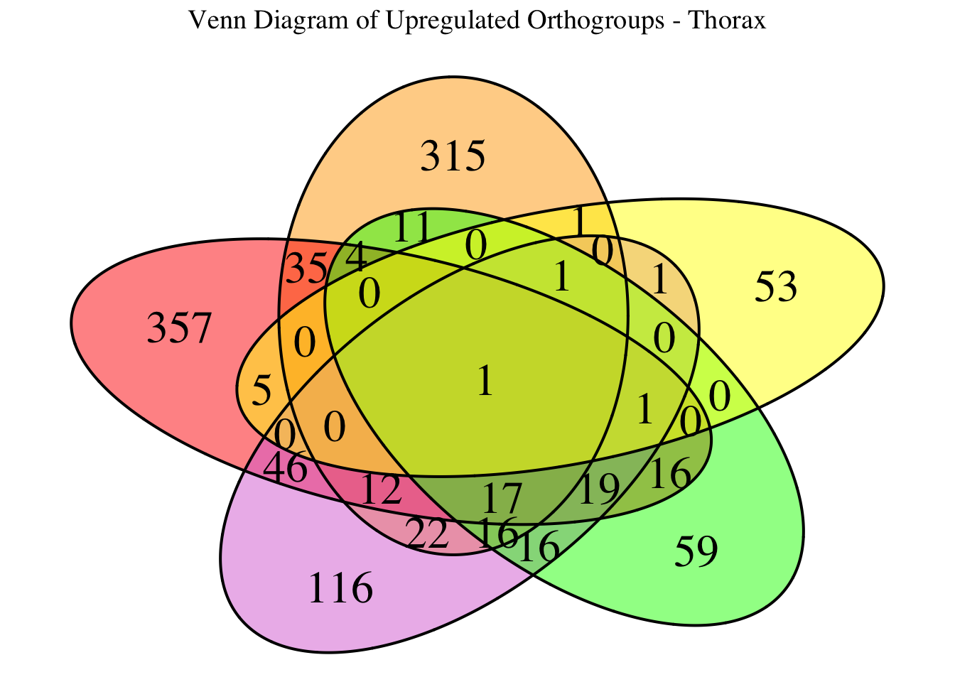
| Version | Author | Date |
|---|---|---|
| b540a1e | Maeva TECHER | 2025-02-27 |
display_venn_with_datatable(venn_data_allspecies_thorax$down, "Venn Diagram of Downregulated Orthogroups - Thorax")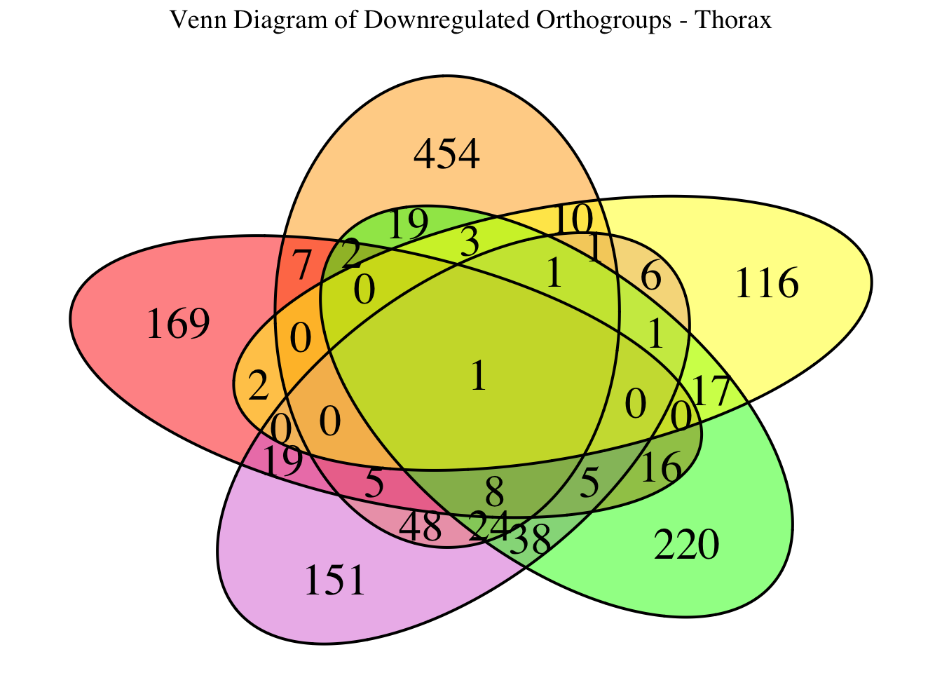
| Version | Author | Date |
|---|---|---|
| b540a1e | Maeva TECHER | 2025-02-27 |
display_venn_with_datatable(venn_data_allspecies_thorax$all, "Venn Diagram of All Significant Orthogroups - Thorax")
| Version | Author | Date |
|---|---|---|
| b540a1e | Maeva TECHER | 2025-02-27 |
# Load Orthogroup information
input_file <- file.path(ortho_dir, "Results_I2/Orthogroups_genesproteinbiotype_Schistocerca_Jan2025.csv")
filtered_final_orthotable <- read.csv(input_file, header = TRUE, stringsAsFactors = FALSE)

# Ensure correct column names
if ("gene_id" %in% colnames(filtered_final_orthotable)) {
  colnames(filtered_final_orthotable)[colnames(filtered_final_orthotable) == "gene_id"] <- "GeneID"
}

# Select relevant columns and ensure uniqueness
filtered_final_orthotable <- filtered_final_orthotable %>%
  select(GeneID, Orthogroup) %>%
  distinct(GeneID, .keep_all = TRUE)  # Keep unique mapping

# Define species order explicitly
species_order <- c("nitens", "cubense", "americana", "piceifrons", "cancellata", "gregaria")

# Initialize an empty list to store heatmap data
heatmap_list <- list()

# Loop through each species to process their Thorax data
for (species in species_order) {
  message(paste("Processing species:", species))

  # Define file path for Thorax
  thorax_file <- file.path(workDir, "DEG_results/Bulk_RNAseq/", paste0(species, "/Thorax/DESeq2_results_Thorax_", species,".csv"))

  # Check if file exists before loading
  if (!file.exists(thorax_file)) {
    message(paste("Missing Thorax file for:", species, "- Assigning empty dataset"))
    thorax_data <- data.frame(GeneID = character(), padj = numeric(), log2FoldChange = numeric(), stringsAsFactors = FALSE)
  } else {
    thorax_data <- tryCatch(read.csv(thorax_file, stringsAsFactors = FALSE), error = function(e) data.frame())
  }

  # Ensure GeneID column exists
  if (!"GeneID" %in% colnames(thorax_data) && "X" %in% colnames(thorax_data)) {
    colnames(thorax_data)[colnames(thorax_data) == "X"] <- "GeneID"
  }

  # Convert GeneID to character
  thorax_data$GeneID <- as.character(thorax_data$GeneID)
  filtered_final_orthotable$GeneID <- as.character(filtered_final_orthotable$GeneID)

  # Merge with orthogroup information
  thorax_data <- left_join(thorax_data, filtered_final_orthotable, by = "GeneID") %>%
    mutate(Orthogroup = ifelse(is.na(Orthogroup), "Unassigned", Orthogroup))

  # If no significant DEGs are found, ensure the structure is correct
  if (nrow(thorax_data) == 0) {
    message(paste("No significant Thorax DEGs for:", species, "- Assigning placeholder values"))
    thorax_data <- data.frame(
      Orthogroup = character(),
      log2FoldChange = numeric(),
      Tissue = character(),
      Regulation = character(),
      Species = character()
    )
  } else {
    # Filter for significant DEGs and select top 500 upregulated and downregulated genes
    thorax_up <- thorax_data %>%
      filter(padj < 0.05 & log2FoldChange > 1) %>%
      arrange(desc(log2FoldChange)) %>%
      slice(1:500)

    thorax_down <- thorax_data %>%
      filter(padj < 0.05 & log2FoldChange < -1) %>%
      arrange(log2FoldChange) %>%
      slice(1:500)

    # Combine data and prepare for heatmap
    thorax_data <- bind_rows(
      thorax_up %>% mutate(Tissue = "Thorax", Regulation = "Upregulated", Species = species),
      thorax_down %>% mutate(Tissue = "Thorax", Regulation = "Downregulated", Species = species)
    ) %>%
      select(Orthogroup, log2FoldChange, Tissue, Regulation, Species)
  }

  # Append to heatmap list, ensuring species is represented
  heatmap_list[[species]] <- thorax_data
}

# Combine all species data
final_heatmap_data <- bind_rows(heatmap_list)

# Ensure all species are represented, even if they have no significant DEGs
for (species in species_order) {
    if (!species %in% unique(final_heatmap_data$Species)) {
        message(paste("Adding placeholder for missing species:", species))
        final_heatmap_data <- bind_rows(
            final_heatmap_data,
            data.frame(
                Orthogroup = "Unassigned",  # Placeholder Orthogroup
                log2FoldChange = 0,
                Tissue = "Thorax",
                Regulation = "None",
                Species = species
            )
        )
    }
}

# Ensure species order in the data
final_heatmap_data$Species <- factor(final_heatmap_data$Species, levels = species_order)

# Create heatmap matrix (Thorax only)
heatmap_matrix <- final_heatmap_data %>%
  group_by(Orthogroup, Species) %>%
  summarize(log2FoldChange = mean(log2FoldChange, na.rm = TRUE), .groups = "drop") %>%
  pivot_wider(names_from = Species, values_from = log2FoldChange, values_fill = 0) %>%
  column_to_rownames("Orthogroup") %>%
  as.matrix()

# Explicitly reorder the columns in heatmap_matrix
heatmap_matrix <- heatmap_matrix[, species_order, drop = FALSE]  # Ensure order is applied

# Define color palettes
custom_cyan_orange_palette <- colorRampPalette(c("cyan", "cyan2", "cyan3", "black", "orange3", "orange2", "orange"))(100)
custom_blue_red_palette <- colorRampPalette(c("blue3", "blue2", "blue1", "white", "red", "red2", "red3"))(100)

# Define color breaks
max_abs_lfc <- max(abs(heatmap_matrix), na.rm = TRUE)
color_breaks <- seq(-max_abs_lfc, max_abs_lfc, length.out = 100)

# Generate heatmaps (Only thorax)
pheatmap(
  heatmap_matrix,
  color = custom_blue_red_palette,
  breaks = color_breaks,
  cluster_rows = TRUE,
  cluster_cols = FALSE,
  show_rownames = FALSE,
  show_colnames = TRUE,
  fontsize_row = 6,
  fontsize_col = 10,
  main = "Heatmap of Orthologs Expression in Thorax Tissue - STRATEGY 2"
)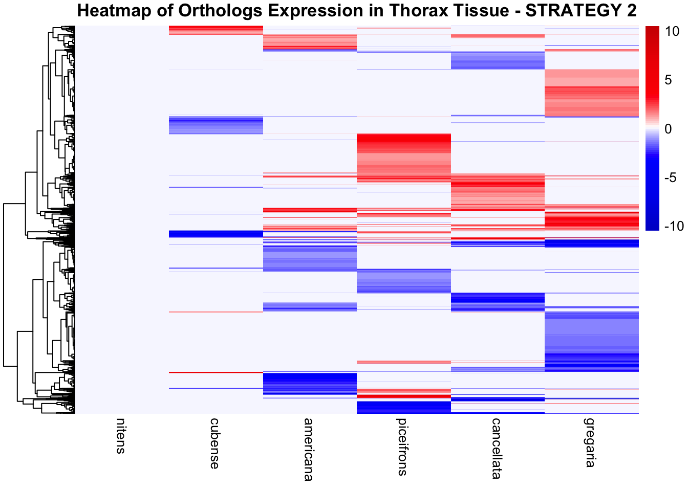
| Version | Author | Date |
|---|---|---|
| b540a1e | Maeva TECHER | 2025-02-27 |
pheatmap(
  heatmap_matrix,
  color = custom_cyan_orange_palette,
  breaks = color_breaks,
  cluster_rows = TRUE,
  cluster_cols = FALSE,
  show_rownames = FALSE,
  show_colnames = TRUE,
  fontsize_row = 6,
  fontsize_col = 10,
  main = "Heatmap of Orthologs Expression in Thorax Tissue - STRATEGY 2"
)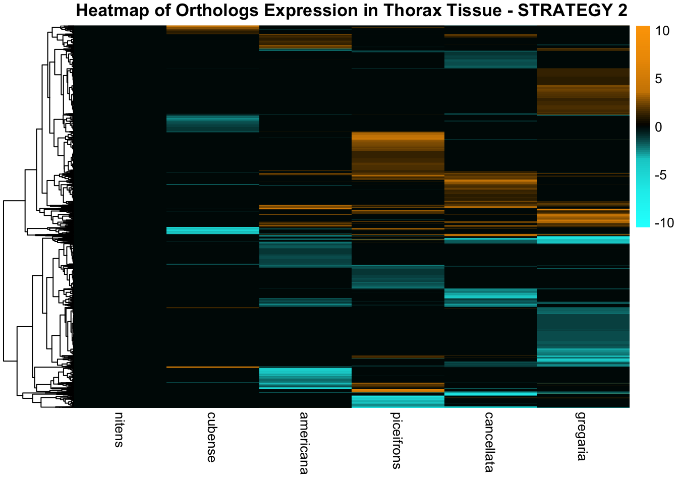
| Version | Author | Date |
|---|---|---|
| b540a1e | Maeva TECHER | 2025-02-27 |
All species
Combined tissues
# Define the species list
allspecies <- c("nitens", "cubense", "americana", "piceifrons", "cancellata", "gregaria")

# Path to the orthogroup mapping file
input_file <- file.path(ortho_dir, "Results_I2/Orthogroups_genesproteinbiotype_Schistocerca_Jan2025.csv")

# Load the orthogroup mapping file
if (!file.exists(input_file)) {
  stop("Error: Orthogroup mapping file not found!")
}
filtered_final_orthotable <- read.csv(input_file, header = TRUE, stringsAsFactors = FALSE)

# Function to load DESeq2 data and map GeneIDs to Orthogroups
load_deseq2_upset_data <- function(tissue) {
  species_deg_list <- list()  # Store significant Orthogroups per species

  for (species in allspecies) {
    # Construct the correct file path
    deg_file <- file.path(workDir, "DEG_results/Bulk_RNAseq", species, tissue,
                          paste0("DESeq2_results_", tissue, "_", species, ".csv"))

    # Skip if file does not exist
    if (!file.exists(deg_file)) {
      message(paste("File missing for species:", species))
      next
    }

    # Load the DESeq2 results file
    deseq_data <- read.csv(deg_file, stringsAsFactors = FALSE)

    # Check for GeneID column
    if (!"GeneID" %in% colnames(deseq_data)) {
      if ("X" %in% colnames(deseq_data)) {
        colnames(deseq_data)[colnames(deseq_data) == "X"] <- "GeneID"
      } else {
        stop(paste("Error: No 'GeneID' column found in", deg_file))
      }
    }

    # Merge DESeq2 results with the orthogroup mapping
    deseq_data_merged <- merge(deseq_data, filtered_final_orthotable[, c("GeneID", "Orthogroup")], by = "GeneID", all.x = TRUE)

    # Handle missing Orthogroups
    deseq_data_merged$Orthogroup[is.na(deseq_data_merged$Orthogroup)] <- "Unknown"

    # Filter for significant DEGs based on Orthogroups
    significant_orthogroups <- deseq_data_merged %>%
      filter(padj < 0.05 & abs(log2FoldChange) >= 1) %>%
      pull(Orthogroup) %>%
      unique()  # Remove duplicates

    # Store the Orthogroup list for the species
    species_deg_list[[species]] <- significant_orthogroups
  }

  # Create a binary matrix for UpSet plot
  all_orthogroups <- unique(unlist(species_deg_list))  # Collect all unique Orthogroups
  upset_data <- data.frame(Orthogroup = all_orthogroups)

  for (species in allspecies) {
    upset_data[[species]] <- as.integer(all_orthogroups %in% species_deg_list[[species]])
  }

  return(upset_data)
}

# Load DEG data based on Orthogroups for Head and Thorax
upset_data_head <- load_deseq2_upset_data("Head")
upset_data_thorax <- load_deseq2_upset_data("Thorax")


# Function to visualize Venn diagram using ggVennDiagram
display_ggvenn_plot <- function(venn_data, title) {
  gg_venn <- ggVennDiagram(venn_data, label_alpha = 0, edge_lty = "dashed") +
    scale_fill_gradient(low = "lightblue", high = "darkblue") +
    labs(title = title) +
    theme_minimal(base_size = 14)

  return(gg_venn)
}

# **Generate Venn diagrams with ORTHOGROUPS**
ggvenn_head_all <- display_ggvenn_plot(venn_data_head$all, "Venn Diagram of All Significant Orthogroups (Head) - All Species")
ggvenn_thorax_all <- display_ggvenn_plot(venn_data_thorax$all, "Venn Diagram of All Significant Orthogroups (Thorax) - All Species")


display_upset_plot <- function(upset_data, title) {
    upset_plot <- upset(
        upset_data,
        allspecies,
        sort_sets = FALSE,
        base_annotations = list(
            'Intersection size' = intersection_size(counts = FALSE) +
                ylab('# Orthogroups in intersection') +
                scale_y_continuous(expand = expansion(mult = c(0, 0.05)))
        ),
        matrix = (
            intersection_matrix(
                geom = geom_point(
                    shape = 'circle',
                    size = 4
                ),
                segment = geom_segment(
                    linetype = 'solid',
                    size = 1
                ),
                outline_color = list(
                    active = 'black',
                    inactive = 'grey80'
                )
            )
        ),
        queries = list(
            upset_query(
                intersect = c('gregaria', 'cancellata'),
                color = 'orange',
                fill = 'orange',
                only_components = c('intersections_matrix', 'Intersection size')
            ),
            upset_query(
                intersect = c('gregaria', 'piceifrons'),
                color = 'orange',
                fill = 'orange',
                only_components = c('intersections_matrix', 'Intersection size')
            ),
            upset_query(
                intersect = c('cancellata', 'piceifrons'),
                color = 'orange',
                fill = 'orange',
                only_components = c('intersections_matrix', 'Intersection size')
            ),
            upset_query(
                intersect = c('gregaria', 'piceifrons', 'cancellata'),
                color = 'darkred',
                fill = 'darkred',
                only_components = c('intersections_matrix', 'Intersection size')
            ),
            upset_query(
                intersect = c('gregaria', 'piceifrons', 'cancellata', 'americana'),
                color = 'purple',
                fill = 'purple',
                only_components = c('intersections_matrix', 'Intersection size')
            ),
            upset_query(set = 'gregaria', fill = 'darkred'),
            upset_query(set = 'piceifrons', fill = 'darkred'),
            upset_query(set = 'cancellata', fill = 'darkred'),
            upset_query(set = 'americana', fill = 'black'),
            upset_query(set = 'cubense', fill = 'black'),
            upset_query(set = 'nitens', fill = 'black')
        ),
        set_sizes = upset_set_size(
            geom = geom_bar(width = 0.8),
            position = 'right'
        ) +
        ylab('# Orthogroups per species') +
        theme(
            axis.line.x = element_line(colour = 'black'),
            axis.ticks.x = element_line()
        ),
        stripes = upset_stripes(
            geom = geom_segment(size = 12),
            colors = c('grey95', 'white')
        )
    ) +
    theme_minimal() +
    theme(
        panel.grid.major = element_blank(),
        panel.grid.minor = element_blank(),
        axis.line = element_line(colour = 'black'),
        text = element_text(size = 14),
        axis.text.x = element_text(face = "italic"),
        plot.title = element_text(hjust = 0.5, face = "bold", size = 16)
    ) +
    ggtitle(title)

    return(upset_plot)
}

# **Generate UpSet plots**
upset_head <- display_upset_plot(upset_data_head, "Intersection from Head")
ggvenn_head_all; print(upset_head)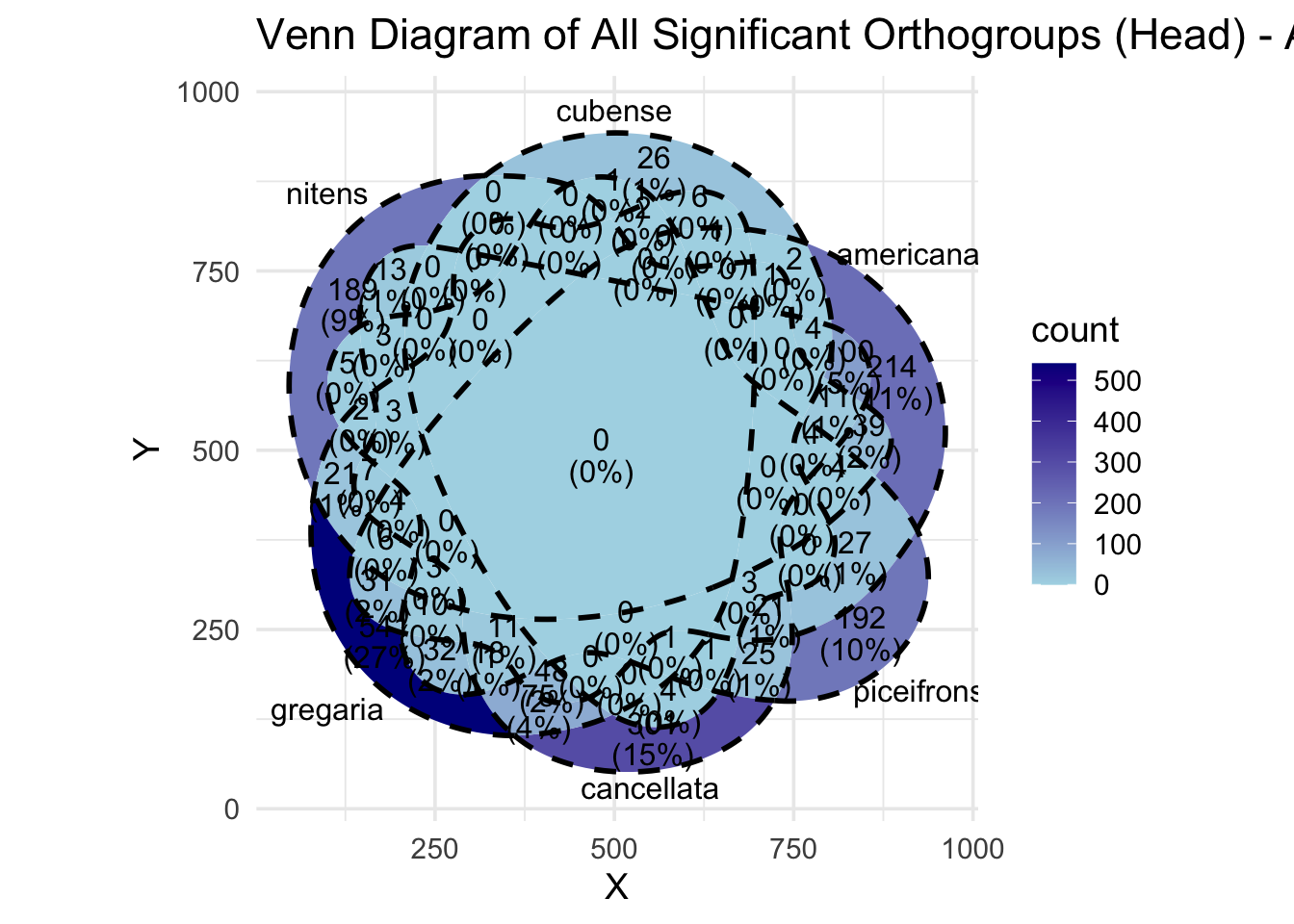
| Version | Author | Date |
|---|---|---|
| b540a1e | Maeva TECHER | 2025-02-27 |
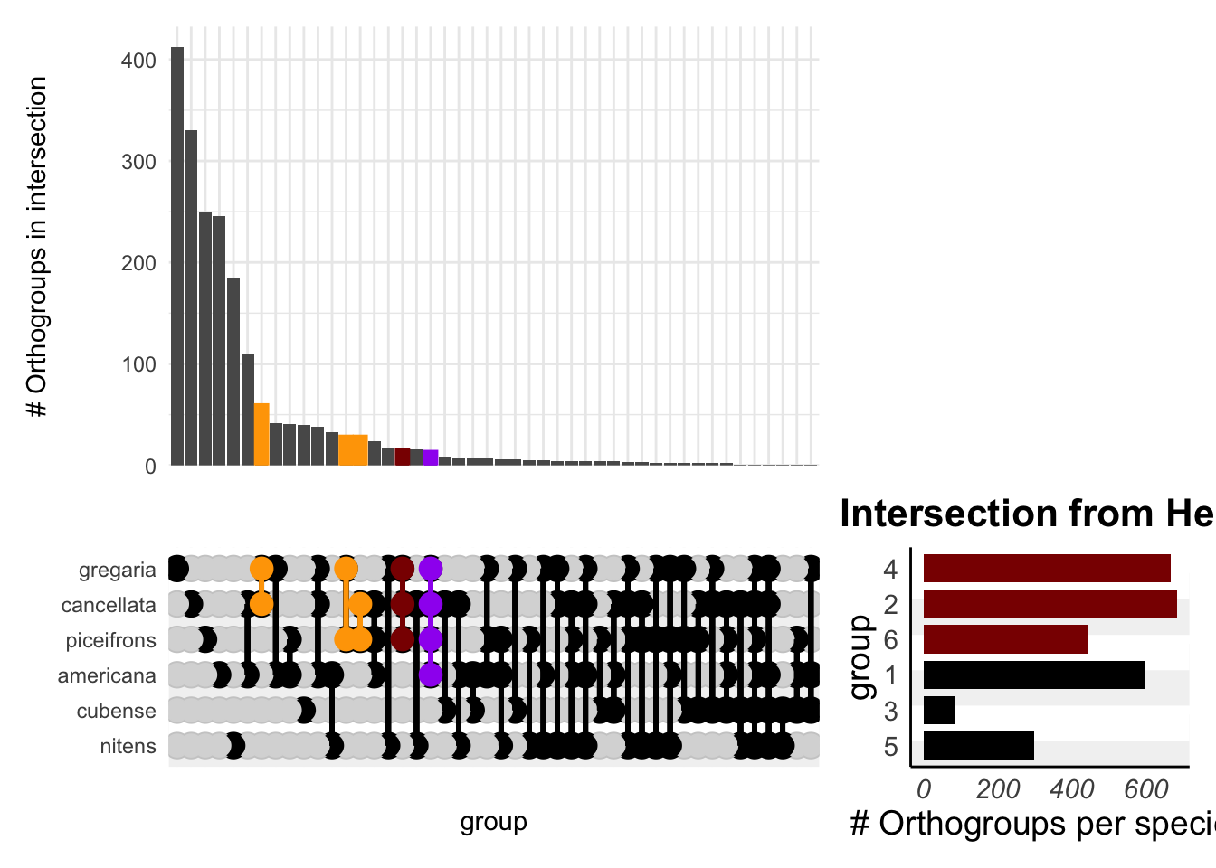
| Version | Author | Date |
|---|---|---|
| b540a1e | Maeva TECHER | 2025-02-27 |
upset_thorax <- display_upset_plot(upset_data_thorax, "Intersection from Thorax")
ggvenn_thorax_all; print(upset_thorax)
| Version | Author | Date |
|---|---|---|
| b540a1e | Maeva TECHER | 2025-02-27 |
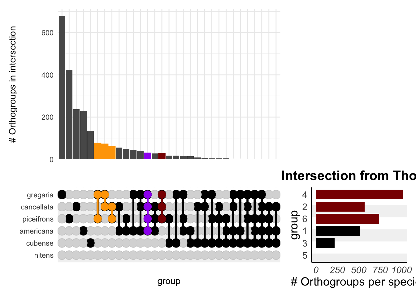
| Version | Author | Date |
|---|---|---|
| b540a1e | Maeva TECHER | 2025-02-27 |
# Function to extract Orthogroups for a specific intersection
extract_orthogroups_from_intersection <- function(upset_data, selected_species) {
    # Ensure the input species exist in the dataset
    selected_species <- intersect(selected_species, colnames(upset_data))

    # Select rows where all selected species have '1' (present in the intersection)
    intersecting_orthogroups <- upset_data[rowSums(upset_data[selected_species]) == length(selected_species), ]

    # Return only the Orthogroups as a DataFrame
    return(data.frame(Orthogroup = intersecting_orthogroups$Orthogroup))
}

shared_orthogroups <- extract_orthogroups_from_intersection(upset_data_head, c("gregaria", "cancellata", "piceifrons"))

kable(shared_orthogroups, col.names = c("Head: shared orthogroups among all locusts")) %>%
kable_styling(bootstrap_options = c("striped", "hover"))| Head: shared orthogroups among all locusts |
|---|
| Unknown |
| OG0009529 |
| OG0000270 |
| OG0000354 |
| OG0000149 |
| OG0004381 |
| OG0000447 |
| OG0011171 |
| OG0005490 |
| OG0003935 |
| OG0000273 |
| OG0000505 |
| OG0007485 |
| OG0004570 |
| OG0008546 |
| OG0000630 |
| OG0009787 |
| OG0010634 |
| OG0013175 |
| OG0010889 |
| OG0010928 |
| OG0001019 |
| OG0005151 |
| OG0002151 |
| OG0000272 |
| OG0013490 |
| OG0008668 |
| OG0014256 |
| OG0012948 |
| OG0000307 |
| OG0000522 |
| OG0008322 |
| OG0000197 |
| OG0009537 |
shared_orthogroups <- extract_orthogroups_from_intersection(upset_data_head, c("gregaria", "cancellata", "piceifrons"))

kable(shared_orthogroups, col.names = c("Head: shared orthogroups among all locusts + americana")) %>%
kable_styling(bootstrap_options = c("striped", "hover"))| Head: shared orthogroups among all locusts + americana |
|---|
| Unknown |
| OG0009529 |
| OG0000270 |
| OG0000354 |
| OG0000149 |
| OG0004381 |
| OG0000447 |
| OG0011171 |
| OG0005490 |
| OG0003935 |
| OG0000273 |
| OG0000505 |
| OG0007485 |
| OG0004570 |
| OG0008546 |
| OG0000630 |
| OG0009787 |
| OG0010634 |
| OG0013175 |
| OG0010889 |
| OG0010928 |
| OG0001019 |
| OG0005151 |
| OG0002151 |
| OG0000272 |
| OG0013490 |
| OG0008668 |
| OG0014256 |
| OG0012948 |
| OG0000307 |
| OG0000522 |
| OG0008322 |
| OG0000197 |
| OG0009537 |
shared_orthogroups <- extract_orthogroups_from_intersection(upset_data_thorax, c("gregaria", "cancellata", "piceifrons"))

kable(shared_orthogroups, col.names = c("Thorax: shared orthogroups among all locusts")) %>%
kable_styling(bootstrap_options = c("striped", "hover"))| Thorax: shared orthogroups among all locusts |
|---|
| Unknown |
| OG0011162 |
| OG0010410 |
| OG0004381 |
| OG0003684 |
| OG0010743 |
| OG0011346 |
| OG0011869 |
| OG0000396 |
| OG0000008 |
| OG0005991 |
| OG0000270 |
| OG0006293 |
| OG0006295 |
| OG0003407 |
| OG0007438 |
| OG0006530 |
| OG0000037 |
| OG0006498 |
| OG0000504 |
| OG0000505 |
| OG0012855 |
| OG0000196 |
| OG0008773 |
| OG0002449 |
| OG0008629 |
| OG0012943 |
| OG0013891 |
| OG0003704 |
| OG0009787 |
| OG0003702 |
| OG0009902 |
| OG0002897 |
| OG0010559 |
| OG0000446 |
| OG0010863 |
| OG0011005 |
| OG0000027 |
| OG0004972 |
| OG0014897 |
| OG0005943 |
| OG0005151 |
| OG0002151 |
| OG0000218 |
| OG0000112 |
| OG0001366 |
| OG0007864 |
| OG0008668 |
| OG0004741 |
| OG0014256 |
| OG0000354 |
| OG0000630 |
| OG0008761 |
| OG0002570 |
| OG0012394 |
| OG0000197 |
| OG0009529 |
| OG0009516 |
shared_orthogroups <- extract_orthogroups_from_intersection(upset_data_thorax, c("gregaria", "cancellata", "piceifrons"))

kable(shared_orthogroups, col.names = c("Thorax: shared orthogroups among all locusts + americana")) %>%
kable_styling(bootstrap_options = c("striped", "hover"))| Thorax: shared orthogroups among all locusts + americana |
|---|
| Unknown |
| OG0011162 |
| OG0010410 |
| OG0004381 |
| OG0003684 |
| OG0010743 |
| OG0011346 |
| OG0011869 |
| OG0000396 |
| OG0000008 |
| OG0005991 |
| OG0000270 |
| OG0006293 |
| OG0006295 |
| OG0003407 |
| OG0007438 |
| OG0006530 |
| OG0000037 |
| OG0006498 |
| OG0000504 |
| OG0000505 |
| OG0012855 |
| OG0000196 |
| OG0008773 |
| OG0002449 |
| OG0008629 |
| OG0012943 |
| OG0013891 |
| OG0003704 |
| OG0009787 |
| OG0003702 |
| OG0009902 |
| OG0002897 |
| OG0010559 |
| OG0000446 |
| OG0010863 |
| OG0011005 |
| OG0000027 |
| OG0004972 |
| OG0014897 |
| OG0005943 |
| OG0005151 |
| OG0002151 |
| OG0000218 |
| OG0000112 |
| OG0001366 |
| OG0007864 |
| OG0008668 |
| OG0004741 |
| OG0014256 |
| OG0000354 |
| OG0000630 |
| OG0008761 |
| OG0002570 |
| OG0012394 |
| OG0000197 |
| OG0009529 |
| OG0009516 |
# **Shared Orthogroups among Gregaria and Piceifrons (Head)**
shared_orthogroups_head_piceifrons_gregaria <- extract_orthogroups_from_intersection(upset_data_head, c("gregaria", "piceifrons"))

kable(shared_orthogroups_head_piceifrons_gregaria, col.names = c("Head: shared orthogroups between gregaria & piceifrons")) %>%
kable_styling(bootstrap_options = c("striped", "hover"))| Head: shared orthogroups between gregaria & piceifrons |
|---|
| Unknown |
| OG0000166 |
| OG0009529 |
| OG0000270 |
| OG0004674 |
| OG0011600 |
| OG0000354 |
| OG0000090 |
| OG0006240 |
| OG0000934 |
| OG0000315 |
| OG0000149 |
| OG0004381 |
| OG0000447 |
| OG0011171 |
| OG0005490 |
| OG0004955 |
| OG0006293 |
| OG0003935 |
| OG0012749 |
| OG0000273 |
| OG0000505 |
| OG0007485 |
| OG0004570 |
| OG0000129 |
| OG0008546 |
| OG0000630 |
| OG0000156 |
| OG0001210 |
| OG0009787 |
| OG0010634 |
| OG0012434 |
| OG0002916 |
| OG0002895 |
| OG0013175 |
| OG0013251 |
| OG0010718 |
| OG0010889 |
| OG0010928 |
| OG0011133 |
| OG0000054 |
| OG0001019 |
| OG0005255 |
| OG0005151 |
| OG0005150 |
| OG0006746 |
| OG0002151 |
| OG0006894 |
| OG0007263 |
| OG0007090 |
| OG0004140 |
| OG0007225 |
| OG0000272 |
| OG0000265 |
| OG0001611 |
| OG0000626 |
| OG0001366 |
| OG0007885 |
| OG0000621 |
| OG0000114 |
| OG0013490 |
| OG0008668 |
| OG0014256 |
| OG0012948 |
| OG0008561 |
| OG0000307 |
| OG0000522 |
| OG0008322 |
| OG0000311 |
| OG0009034 |
| OG0013039 |
| OG0000197 |
| OG0009646 |
| OG0000830 |
| OG0009537 |
| OG0009622 |
# **Shared Orthogroups among Piceifrons and Cancellata (Head)**
shared_orthogroups_head_piceifrons_cancellata <- extract_orthogroups_from_intersection(upset_data_head, c("piceifrons", "cancellata"))

kable(shared_orthogroups_head_piceifrons_cancellata, col.names = c("Head: shared orthogroups between piceifrons & cancellata")) %>%
kable_styling(bootstrap_options = c("striped", "hover"))| Head: shared orthogroups between piceifrons & cancellata |
|---|
| Unknown |
| OG0009529 |
| OG0004972 |
| OG0000270 |
| OG0011387 |
| OG0011869 |
| OG0006739 |
| OG0006438 |
| OG0000354 |
| OG0008632 |
| OG0008567 |
| OG0000002 |
| OG0006291 |
| OG0000032 |
| OG0008500 |
| OG0000149 |
| OG0004381 |
| OG0000447 |
| OG0011199 |
| OG0011171 |
| OG0011248 |
| OG0003815 |
| OG0005490 |
| OG0005694 |
| OG0000757 |
| OG0005297 |
| OG0012624 |
| OG0003935 |
| OG0003407 |
| OG0007438 |
| OG0000154 |
| OG0006411 |
| OG0000273 |
| OG0006934 |
| OG0000505 |
| OG0002273 |
| OG0007485 |
| OG0012855 |
| OG0007756 |
| OG0002241 |
| OG0004570 |
| OG0000063 |
| OG0008946 |
| OG0012946 |
| OG0008546 |
| OG0000630 |
| OG0008550 |
| OG0013908 |
| OG0004857 |
| OG0002618 |
| OG0009787 |
| OG0000573 |
| OG0010634 |
| OG0013150 |
| OG0010430 |
| OG0000440 |
| OG0010233 |
| OG0000843 |
| OG0010513 |
| OG0013175 |
| OG0010889 |
| OG0010928 |
| OG0014066 |
| OG0013300 |
| OG0000093 |
| OG0003126 |
| OG0000033 |
| OG0011499 |
| OG0001019 |
| OG0004341 |
| OG0005274 |
| OG0001009 |
| OG0005772 |
| OG0005151 |
| OG0000045 |
| OG0000600 |
| OG0000372 |
| OG0002151 |
| OG0013772 |
| OG0000272 |
| OG0000112 |
| OG0007484 |
| OG0008072 |
| OG0007610 |
| OG0000624 |
| OG0013490 |
| OG0008668 |
| OG0014256 |
| OG0012948 |
| OG0000307 |
| OG0000522 |
| OG0008322 |
| OG0000197 |
| OG0010012 |
| OG0002716 |
| OG0009517 |
| OG0009537 |
| OG0000824 |
# **Shared Orthogroups among Cancellata and Gregaria (Head)**
shared_orthogroups_head_cancellata_gregaria <- extract_orthogroups_from_intersection(upset_data_head, c("cancellata", "gregaria"))

kable(shared_orthogroups_head_cancellata_gregaria, col.names = c("Head: shared orthogroups between cancellata & gregaria")) %>%
kable_styling(bootstrap_options = c("striped", "hover"))| Head: shared orthogroups between cancellata & gregaria |
|---|
| Unknown |
| OG0009529 |
| OG0015091 |
| OG0003125 |
| OG0000169 |
| OG0000111 |
| OG0000270 |
| OG0012003 |
| OG0004199 |
| OG0000354 |
| OG0008543 |
| OG0012986 |
| OG0008460 |
| OG0000022 |
| OG0000428 |
| OG0000149 |
| OG0010418 |
| OG0002873 |
| OG0010643 |
| OG0010433 |
| OG0004381 |
| OG0004715 |
| OG0010744 |
| OG0000446 |
| OG0000447 |
| OG0011171 |
| OG0011005 |
| OG0003242 |
| OG0011451 |
| OG0011450 |
| OG0005782 |
| OG0000404 |
| OG0005566 |
| OG0005490 |
| OG0005216 |
| OG0006216 |
| OG0006295 |
| OG0003810 |
| OG0003935 |
| OG0007329 |
| OG0007332 |
| OG0007328 |
| OG0000781 |
| OG0007343 |
| OG0007330 |
| OG0006530 |
| OG0000038 |
| OG0006881 |
| OG0000418 |
| OG0000504 |
| OG0000273 |
| OG0007331 |
| OG0000505 |
| OG0007340 |
| OG0006883 |
| OG0007342 |
| OG0007485 |
| OG0007837 |
| OG0004570 |
| OG0008773 |
| OG0008549 |
| OG0008546 |
| OG0000630 |
| OG0012943 |
| OG0009863 |
| OG0009787 |
| OG0010634 |
| OG0013175 |
| OG0010889 |
| OG0010928 |
| OG0001019 |
| OG0005151 |
| OG0002151 |
| OG0000272 |
| OG0013490 |
| OG0008668 |
| OG0014256 |
| OG0012948 |
| OG0000307 |
| OG0000522 |
| OG0008322 |
| OG0000197 |
| OG0009537 |
| OG0008573 |
| OG0004675 |
| OG0002647 |
| OG0000882 |
| OG0010416 |
| OG0010421 |
| OG0010142 |
| OG0010264 |
| OG0010414 |
| OG0014280 |
| OG0010415 |
| OG0010437 |
| OG0000200 |
| OG0000202 |
| OG0000229 |
| OG0010966 |
| OG0014294 |
| OG0010772 |
| OG0000057 |
| OG0011222 |
| OG0011093 |
| OG0014897 |
| OG0005668 |
| OG0001037 |
| OG0000601 |
| OG0000599 |
| OG0013443 |
| OG0001488 |
| OG0005949 |
| OG0000124 |
| OG0005279 |
| OG0000577 |
| OG0003360 |
| OG0012394 |
| OG0007023 |
| OG0001453 |
| OG0012762 |
| OG0000611 |
| OG0014210 |
| OG0000218 |
| OG0014212 |
| OG0007266 |
| OG0007275 |
| OG0014928 |
| OG0001100 |
| OG0003844 |
| OG0007421 |
| OG0004079 |
| OG0011757 |
| OG0007839 |
| OG0007458 |
| OG0007611 |
| OG0015939 |
| OG0007975 |
| OG0012865 |
| OG0008761 |
| OG0000196 |
| OG0008973 |
| OG0013013 |
| OG0008353 |
# **Shared Orthogroups among Gregaria and Piceifrons (Thorax)**
shared_orthogroups_thorax_piceifrons_gregaria <- extract_orthogroups_from_intersection(upset_data_thorax, c("gregaria", "piceifrons"))

kable(shared_orthogroups_thorax_piceifrons_gregaria, col.names = c("Thorax: shared orthogroups between gregaria & piceifrons")) %>%
kable_styling(bootstrap_options = c("striped", "hover"))| Thorax: shared orthogroups between gregaria & piceifrons |
|---|
| Unknown |
| OG0010450 |
| OG0000315 |
| OG0003108 |
| OG0011162 |
| OG0005448 |
| OG0011755 |
| OG0004286 |
| OG0010350 |
| OG0010410 |
| OG0010691 |
| OG0004381 |
| OG0003684 |
| OG0010743 |
| OG0011171 |
| OG0011346 |
| OG0011869 |
| OG0011779 |
| OG0012085 |
| OG0001685 |
| OG0000396 |
| OG0012567 |
| OG0000008 |
| OG0005146 |
| OG0012678 |
| OG0005991 |
| OG0000270 |
| OG0006293 |
| OG0006295 |
| OG0000031 |
| OG0012376 |
| OG0003407 |
| OG0007438 |
| OG0002206 |
| OG0006530 |
| OG0000037 |
| OG0006498 |
| OG0000504 |
| OG0000505 |
| OG0012855 |
| OG0000196 |
| OG0008773 |
| OG0002449 |
| OG0008629 |
| OG0012943 |
| OG0013891 |
| OG0009355 |
| OG0003423 |
| OG0003704 |
| OG0009787 |
| OG0003702 |
| OG0009902 |
| OG0002897 |
| OG0010425 |
| OG0010559 |
| OG0010234 |
| OG0010219 |
| OG0002895 |
| OG0000200 |
| OG0010900 |
| OG0000446 |
| OG0010889 |
| OG0001263 |
| OG0013232 |
| OG0010966 |
| OG0010863 |
| OG0013543 |
| OG0011005 |
| OG0011092 |
| OG0011133 |
| OG0000319 |
| OG0000027 |
| OG0000561 |
| OG0003126 |
| OG0011312 |
| OG0011771 |
| OG0011437 |
| OG0011384 |
| OG0014481 |
| OG0012682 |
| OG0000059 |
| OG0001826 |
| OG0003370 |
| OG0005531 |
| OG0005626 |
| OG0001920 |
| OG0005398 |
| OG0004972 |
| OG0001723 |
| OG0014897 |
| OG0005062 |
| OG0000395 |
| OG0005937 |
| OG0005371 |
| OG0005943 |
| OG0006288 |
| OG0005151 |
| OG0005150 |
| OG0000265 |
| OG0000149 |
| OG0012779 |
| OG0007374 |
| OG0007266 |
| OG0002151 |
| OG0007330 |
| OG0014210 |
| OG0006894 |
| OG0007121 |
| OG0004199 |
| OG0007329 |
| OG0000218 |
| OG0006857 |
| OG0000112 |
| OG0001100 |
| OG0007413 |
| OG0000574 |
| OG0000626 |
| OG0001366 |
| OG0007864 |
| OG0012856 |
| OG0007885 |
| OG0000114 |
| OG0013490 |
| OG0008668 |
| OG0004741 |
| OG0014256 |
| OG0000354 |
| OG0000307 |
| OG0008796 |
| OG0008775 |
| OG0008772 |
| OG0000630 |
| OG0008763 |
| OG0008761 |
| OG0012994 |
| OG0008630 |
| OG0004880 |
| OG0002570 |
| OG0000220 |
| OG0009361 |
| OG0000311 |
| OG0009440 |
| OG0012394 |
| OG0000156 |
| OG0000197 |
| OG0009863 |
| OG0009529 |
| OG0009544 |
| OG0009516 |
| OG0009646 |
| OG0000830 |
| OG0014387 |
| OG0009648 |
| OG0001210 |
# **Shared Orthogroups among Piceifrons and Cancellata (Thorax)**
shared_orthogroups_thorax_piceifrons_cancellata <- extract_orthogroups_from_intersection(upset_data_thorax, c("piceifrons", "cancellata"))

kable(shared_orthogroups_thorax_piceifrons_cancellata, col.names = c("Thorax: shared orthogroups between piceifrons & cancellata")) %>%
kable_styling(bootstrap_options = c("striped", "hover"))| Thorax: shared orthogroups between piceifrons & cancellata |
|---|
| Unknown |
| OG0004747 |
| OG0000002 |
| OG0011162 |
| OG0000111 |
| OG0012141 |
| OG0000022 |
| OG0010640 |
| OG0013203 |
| OG0010642 |
| OG0002945 |
| OG0010638 |
| OG0010639 |
| OG0010635 |
| OG0002936 |
| OG0010410 |
| OG0004381 |
| OG0003684 |
| OG0010743 |
| OG0000228 |
| OG0000009 |
| OG0011346 |
| OG0011869 |
| OG0012140 |
| OG0005281 |
| OG0005181 |
| OG0000396 |
| OG0003598 |
| OG0000008 |
| OG0006130 |
| OG0005991 |
| OG0000729 |
| OG0001957 |
| OG0000270 |
| OG0006291 |
| OG0006293 |
| OG0006295 |
| OG0003379 |
| OG0003407 |
| OG0006438 |
| OG0007438 |
| OG0000154 |
| OG0006936 |
| OG0006530 |
| OG0000037 |
| OG0006498 |
| OG0000504 |
| OG0006934 |
| OG0007152 |
| OG0000505 |
| OG0012855 |
| OG0000308 |
| OG0000196 |
| OG0008773 |
| OG0002449 |
| OG0008629 |
| OG0012943 |
| OG0008632 |
| OG0013891 |
| OG0002665 |
| OG0009088 |
| OG0003704 |
| OG0009787 |
| OG0003702 |
| OG0009902 |
| OG0000573 |
| OG0002841 |
| OG0010430 |
| OG0002897 |
| OG0010559 |
| OG0002896 |
| OG0001149 |
| OG0010233 |
| OG0000444 |
| OG0010590 |
| OG0004378 |
| OG0004531 |
| OG0000446 |
| OG0010863 |
| OG0011005 |
| OG0011049 |
| OG0000027 |
| OG0000557 |
| OG0000093 |
| OG0000546 |
| OG0000096 |
| OG0000033 |
| OG0012154 |
| OG0011546 |
| OG0005998 |
| OG0000589 |
| OG0005157 |
| OG0004972 |
| OG0000485 |
| OG0014879 |
| OG0006317 |
| OG0001041 |
| OG0014897 |
| OG0012680 |
| OG0005694 |
| OG0006159 |
| OG0005932 |
| OG0000978 |
| OG0005377 |
| OG0005943 |
| OG0005990 |
| OG0005134 |
| OG0005151 |
| OG0002151 |
| OG0006489 |
| OG0007296 |
| OG0014940 |
| OG0000218 |
| OG0006962 |
| OG0000112 |
| OG0007156 |
| OG0007611 |
| OG0008072 |
| OG0012835 |
| OG0012909 |
| OG0001366 |
| OG0007864 |
| OG0007485 |
| OG0003880 |
| OG0007919 |
| OG0008070 |
| OG0000210 |
| OG0013429 |
| OG0008397 |
| OG0008668 |
| OG0008723 |
| OG0004741 |
| OG0014256 |
| OG0000354 |
| OG0008921 |
| OG0001167 |
| OG0000630 |
| OG0008761 |
| OG0008322 |
| OG0004891 |
| OG0002570 |
| OG0009428 |
| OG0012394 |
| OG0000197 |
| OG0009529 |
| OG0010012 |
| OG0009516 |
| OG0009804 |
| OG0002716 |
| OG0009517 |
# **Shared Orthogroups among Cancellata and Gregaria (Thorax)**
shared_orthogroups_thorax_cancellata_gregaria <- extract_orthogroups_from_intersection(upset_data_thorax, c("cancellata", "gregaria"))

kable(shared_orthogroups_thorax_cancellata_gregaria, col.names = c("Thorax: shared orthogroups between cancellata & gregaria")) %>%
kable_styling(bootstrap_options = c("striped", "hover"))| Thorax: shared orthogroups between cancellata & gregaria |
|---|
| OG0000282 |
| Unknown |
| OG0014282 |
| OG0003125 |
| OG0011162 |
| OG0001867 |
| OG0003417 |
| OG0000046 |
| OG0007837 |
| OG0004332 |
| OG0010340 |
| OG0010420 |
| OG0010429 |
| OG0010257 |
| OG0010643 |
| OG0010410 |
| OG0004381 |
| OG0003684 |
| OG0004735 |
| OG0010776 |
| OG0010743 |
| OG0010744 |
| OG0011346 |
| OG0011466 |
| OG0003815 |
| OG0011940 |
| OG0011638 |
| OG0011869 |
| OG0012125 |
| OG0011449 |
| OG0011450 |
| OG0011530 |
| OG0005782 |
| OG0000396 |
| OG0005832 |
| OG0005992 |
| OG0005429 |
| OG0005353 |
| OG0001009 |
| OG0000008 |
| OG0005991 |
| OG0000270 |
| OG0006293 |
| OG0006295 |
| OG0003935 |
| OG0003407 |
| OG0007438 |
| OG0006682 |
| OG0007328 |
| OG0007239 |
| OG0006411 |
| OG0007153 |
| OG0001098 |
| OG0006530 |
| OG0000037 |
| OG0006498 |
| OG0000504 |
| OG0001068 |
| OG0000505 |
| OG0000038 |
| OG0004169 |
| OG0012855 |
| OG0007559 |
| OG0000196 |
| OG0008574 |
| OG0008773 |
| OG0008760 |
| OG0002449 |
| OG0008629 |
| OG0008374 |
| OG0012943 |
| OG0008972 |
| OG0013891 |
| OG0001391 |
| OG0003704 |
| OG0009787 |
| OG0003702 |
| OG0013213 |
| OG0009902 |
| OG0002897 |
| OG0010559 |
| OG0000446 |
| OG0010863 |
| OG0011005 |
| OG0000027 |
| OG0004972 |
| OG0014897 |
| OG0005943 |
| OG0005151 |
| OG0002151 |
| OG0000218 |
| OG0000112 |
| OG0001366 |
| OG0007864 |
| OG0008668 |
| OG0004741 |
| OG0014256 |
| OG0000354 |
| OG0000630 |
| OG0008761 |
| OG0002570 |
| OG0012394 |
| OG0000197 |
| OG0009529 |
| OG0009516 |
| OG0008903 |
| OG0004570 |
| OG0001611 |
| OG0004049 |
| OG0004675 |
| OG0009412 |
| OG0002647 |
| OG0001661 |
| OG0000335 |
| OG0000157 |
| OG0009864 |
| OG0001221 |
| OG0002937 |
| OG0013151 |
| OG0010418 |
| OG0013158 |
| OG0010360 |
| OG0010142 |
| OG0000441 |
| OG0004270 |
| OG0010411 |
| OG0010415 |
| OG0000202 |
| OG0000229 |
| OG0000201 |
| OG0014294 |
| OG0010858 |
| OG0010872 |
| OG0011222 |
| OG0003110 |
| OG0015091 |
| OG0003103 |
| OG0003078 |
| OG0001392 |
| OG0004896 |
| OG0001933 |
| OG0005375 |
| OG0003569 |
| OG0005173 |
| OG0006216 |
| OG0006207 |
| OG0000601 |
| OG0000599 |
| OG0005949 |
| OG0005906 |
| OG0001019 |
| OG0005378 |
| OG0005279 |
| OG0005172 |
| OG0001733 |
| OG0007010 |
| OG0000611 |
| OG0006908 |
| OG0006665 |
| OG0013463 |
| OG0013428 |
| OG0007340 |
| OG0000273 |
| OG0007332 |
| OG0011451 |
| OG0003242 |
| OG0012284 |
| OG0007908 |
| OG0008037 |
| OG0008285 |
| OG0015939 |
| OG0007975 |
| OG0012865 |
| OG0013013 |
| OG0008770 |
| OG0008402 |
| OG0008353 |
sessionInfo()R version 4.4.2 (2024-10-31)
Platform: aarch64-apple-darwin20
Running under: macOS Sequoia 15.3
Matrix products: default
BLAS: /Library/Frameworks/R.framework/Versions/4.4-arm64/Resources/lib/libRblas.0.dylib
LAPACK: /Library/Frameworks/R.framework/Versions/4.4-arm64/Resources/lib/libRlapack.dylib; LAPACK version 3.12.0
locale:
[1] en_US.UTF-8/en_US.UTF-8/en_US.UTF-8/C/en_US.UTF-8/en_US.UTF-8
time zone: Asia/Tokyo
tzcode source: internal
attached base packages:
[1] grid stats graphics grDevices utils datasets methods
[8] base
other attached packages:
[1] ComplexUpset_1.3.6 UpSetR_1.4.0 data.table_1.17.0
[4] lubridate_1.9.4 forcats_1.0.0 stringr_1.5.1
[7] purrr_1.0.4 tidyverse_2.0.0 readr_2.1.5
[10] DT_0.33 gridExtra_2.3 VennDiagram_1.7.3
[13] futile.logger_1.4.3 tibble_3.2.1 kableExtra_1.4.0
[16] viridis_0.6.5 viridisLite_0.4.2 RColorBrewer_1.1-3
[19] tidyr_1.3.1 pheatmap_1.0.12 ggVennDiagram_1.5.2
[22] htmlwidgets_1.6.4 plotly_4.10.4 ggplot2_3.5.1
[25] dplyr_1.1.4 knitr_1.49 workflowr_1.7.1
loaded via a namespace (and not attached):
[1] gtable_0.3.6 xfun_0.51 bslib_0.9.0
[4] processx_3.8.6 tzdb_0.4.0 callr_3.7.6
[7] crosstalk_1.2.1 vctrs_0.6.5 tools_4.4.2
[10] ps_1.9.0 generics_0.1.3 pkgconfig_2.0.3
[13] lifecycle_1.0.4 farver_2.1.2 compiler_4.4.2
[16] git2r_0.35.0 textshaping_1.0.0 munsell_0.5.1
[19] getPass_0.2-4 httpuv_1.6.15 htmltools_0.5.8.1
[22] sass_0.4.9 yaml_2.3.10 lazyeval_0.2.2
[25] later_1.4.1 pillar_1.10.1 jquerylib_0.1.4
[28] whisker_0.4.1 cachem_1.1.0 tidyselect_1.2.1
[31] digest_0.6.37 stringi_1.8.4 labeling_0.4.3
[34] rprojroot_2.0.4 fastmap_1.2.0 colorspace_2.1-1
[37] cli_3.6.4 magrittr_2.0.3 patchwork_1.3.0
[40] withr_3.0.2 scales_1.3.0 promises_1.3.2
[43] timechange_0.3.0 rmarkdown_2.29 lambda.r_1.2.4
[46] httr_1.4.7 ragg_1.3.3 hms_1.1.3
[49] evaluate_1.0.3 rlang_1.1.5 futile.options_1.0.1
[52] Rcpp_1.0.14 glue_1.8.0 formatR_1.14
[55] xml2_1.3.6 svglite_2.1.3 rstudioapi_0.17.1
[58] jsonlite_1.9.0 plyr_1.8.9 R6_2.6.1
[61] systemfonts_1.2.1 fs_1.6.5