Signatures of selection: Did locusts or specific genes experience positive selection?
Maeva Techer
2025-09-04
Last updated: 2025-09-04
Checks: 5 2
Knit directory:
locust-comparative-genomics/
This reproducible R Markdown analysis was created with workflowr (version 1.7.1). The Checks tab describes the reproducibility checks that were applied when the results were created. The Past versions tab lists the development history.
The R Markdown file has unstaged changes. To know which version of
the R Markdown file created these results, you’ll want to first commit
it to the Git repo. If you’re still working on the analysis, you can
ignore this warning. When you’re finished, you can run
wflow_publish to commit the R Markdown file and build the
HTML.
Great job! The global environment was empty. Objects defined in the global environment can affect the analysis in your R Markdown file in unknown ways. For reproduciblity it’s best to always run the code in an empty environment.
The command set.seed(20221025) was run prior to running
the code in the R Markdown file. Setting a seed ensures that any results
that rely on randomness, e.g. subsampling or permutations, are
reproducible.
Great job! Recording the operating system, R version, and package versions is critical for reproducibility.
Nice! There were no cached chunks for this analysis, so you can be confident that you successfully produced the results during this run.
Using absolute paths to the files within your workflowr project makes it difficult for you and others to run your code on a different machine. Change the absolute path(s) below to the suggested relative path(s) to make your code more reproducible.
| absolute | relative |
|---|---|
| /Users/maevatecher/Documents/GitHub/locust-comparative-genomics/data/orthofinder/Polyneoptera | data/orthofinder/Polyneoptera |
| /Users/maevatecher/Documents/GitHub/locust-comparative-genomics/data/HYPHY_selection | data/HYPHY_selection |
| /Users/maevatecher/Documents/GitHub/locust-comparative-genomics/data | data |
Great! You are using Git for version control. Tracking code development and connecting the code version to the results is critical for reproducibility.
The results in this page were generated with repository version 05239ca. See the Past versions tab to see a history of the changes made to the R Markdown and HTML files.
Note that you need to be careful to ensure that all relevant files for
the analysis have been committed to Git prior to generating the results
(you can use wflow_publish or
wflow_git_commit). workflowr only checks the R Markdown
file, but you know if there are other scripts or data files that it
depends on. Below is the status of the Git repository when the results
were generated:
Ignored files:
    Ignored:    .DS_Store
    Ignored:    .Rhistory
    Ignored:    analysis/.DS_Store
    Ignored:    analysis/.Rhistory
    Ignored:    analysis/figure/
    Ignored:    code/.DS_Store
    Ignored:    code/scripts/.DS_Store
    Ignored:    code/scripts/pal2nal.v14/.DS_Store
    Ignored:    data/.DS_Store
    Ignored:    data/DEG_results/.DS_Store
    Ignored:    data/DEG_results/Bulk_RNAseq/.DS_Store
    Ignored:    data/DEG_results/Bulk_RNAseq/americana/.DS_Store
    Ignored:    data/DEG_results/Bulk_RNAseq/cancellata/.DS_Store
    Ignored:    data/DEG_results/Bulk_RNAseq/cubense/.DS_Store
    Ignored:    data/DEG_results/Bulk_RNAseq/gregaria/.DS_Store
    Ignored:    data/DEG_results/Bulk_RNAseq/nitens/.DS_Store
    Ignored:    data/HYPHY_selection/.DS_Store
    Ignored:    data/HYPHY_selection/ParsedABSRELResults_unlabeled/
    Ignored:    data/HYPHY_selection/pathway_enrichment/.DS_Store
    Ignored:    data/HYPHY_selection/pathway_enrichment/americana/
    Ignored:    data/HYPHY_selection/pathway_enrichment/cancellata/
    Ignored:    data/HYPHY_selection/pathway_enrichment/cubense/
    Ignored:    data/HYPHY_selection/pathway_enrichment/nitens/
    Ignored:    data/HYPHY_selection/pathway_enrichment/piceifrons/
    Ignored:    data/WGCNA/.DS_Store
    Ignored:    data/WGCNA/input/.DS_Store
    Ignored:    data/WGCNA/input/Bulk_RNAseq/.DS_Store
    Ignored:    data/WGCNA/output/.DS_Store
    Ignored:    data/WGCNA/output/Bulk_RNAseq/.DS_Store
    Ignored:    data/WGCNA/output/Bulk_RNAseq/gregaria/.DS_Store
    Ignored:    data/behavioral_data/.DS_Store
    Ignored:    data/behavioral_data/Raw_data/.DS_Store
    Ignored:    data/cafe5_results/.DS_Store
    Ignored:    data/list/.DS_Store
    Ignored:    data/list/Bulk_RNAseq/.DS_Store
    Ignored:    data/list/GO_Annotations/.DS_Store
    Ignored:    data/list/GO_Annotations/DesertLocustR/.DS_Store
    Ignored:    data/list/excluded_loci/.DS_Store
    Ignored:    data/orthofinder/.DS_Store
    Ignored:    data/orthofinder/Polyneoptera/.DS_Store
    Ignored:    data/orthofinder/Polyneoptera/Results_I2_iqtree/.DS_Store
    Ignored:    data/orthofinder/Polyneoptera/Results_I2_iqtree/Orthogroups/.DS_Store
    Ignored:    data/orthofinder/Polyneoptera/Results_I2_withDaust/.DS_Store
    Ignored:    data/orthofinder/Polyneoptera/Results_I2_withDaust/Orthogroups/.DS_Store
    Ignored:    data/orthofinder/Schistocerca/.DS_Store
    Ignored:    data/orthofinder/Schistocerca/Results_I2/.DS_Store
    Ignored:    data/orthofinder/Schistocerca/Results_I2/Orthogroups/.DS_Store
    Ignored:    data/overlap/.DS_Store
    Ignored:    data/pathway_enrichment/.DS_Store
    Ignored:    data/pathway_enrichment/OLD/.DS_Store
    Ignored:    data/pathway_enrichment/OLD/custom_sgregaria_orgdb/.DS_Store
    Ignored:    data/pathway_enrichment/REVIGO_results/.DS_Store
    Ignored:    data/pathway_enrichment/REVIGO_results/BP/.DS_Store
    Ignored:    data/pathway_enrichment/REVIGO_results/CC/.DS_Store
    Ignored:    data/pathway_enrichment/REVIGO_results/MF/.DS_Store
    Ignored:    data/pathway_enrichment/cancellata/.DS_Store
    Ignored:    data/pathway_enrichment/gregaria/.DS_Store
    Ignored:    data/pathway_enrichment/nitens/Thorax/
    Ignored:    data/pathway_enrichment/piceifrons/.DS_Store
    Ignored:    data/readcounts/.DS_Store
    Ignored:    data/readcounts/Bulk_RNAseq/.DS_Store
    Ignored:    data/readcounts/RNAi/.DS_Store

Untracked files:
    Untracked:  data/RefSeq/

Unstaged changes:
    Modified:   analysis/2_psmc-analysis.Rmd
    Modified:   analysis/2_signatures-selection.Rmd
    Modified:   data/DEG_results/Bulk_RNAseq/americana/Head/heatmap_VST_Head.pdf
    Modified:   data/DEG_results/Bulk_RNAseq/americana/Head/heatmap_VST_Head_togregaria.pdf
    Modified:   data/DEG_results/Bulk_RNAseq/americana/Head/heatmap_normTransform_Head.pdf
    Modified:   data/DEG_results/Bulk_RNAseq/americana/Head/heatmap_normTransform_Head_togregaria.pdf
    Modified:   data/DEG_results/Bulk_RNAseq/americana/Head/heatmap_rlog_Head.pdf
    Modified:   data/DEG_results/Bulk_RNAseq/americana/Head/heatmap_rlog_Head_togregaria.pdf
    Modified:   data/DEG_results/Bulk_RNAseq/americana/Thorax/heatmap_VST_Thorax.pdf
    Modified:   data/DEG_results/Bulk_RNAseq/americana/Thorax/heatmap_VST_Thorax_togregaria.pdf
    Modified:   data/DEG_results/Bulk_RNAseq/americana/Thorax/heatmap_normTransform_Thorax.pdf
    Modified:   data/DEG_results/Bulk_RNAseq/americana/Thorax/heatmap_normTransform_Thorax_togregaria.pdf
    Modified:   data/DEG_results/Bulk_RNAseq/americana/Thorax/heatmap_rlog_Thorax.pdf
    Modified:   data/DEG_results/Bulk_RNAseq/americana/Thorax/heatmap_rlog_Thorax_togregaria.pdf
    Modified:   data/DEG_results/Bulk_RNAseq/cancellata/Head/heatmap_VST_Head.pdf
    Modified:   data/DEG_results/Bulk_RNAseq/cancellata/Head/heatmap_VST_Head_togregaria.pdf
    Modified:   data/DEG_results/Bulk_RNAseq/cancellata/Head/heatmap_normTransform_Head.pdf
    Modified:   data/DEG_results/Bulk_RNAseq/cancellata/Head/heatmap_normTransform_Head_togregaria.pdf
    Modified:   data/DEG_results/Bulk_RNAseq/cancellata/Head/heatmap_rlog_Head.pdf
    Modified:   data/DEG_results/Bulk_RNAseq/cancellata/Head/heatmap_rlog_Head_togregaria.pdf
    Modified:   data/DEG_results/Bulk_RNAseq/cancellata/Thorax/heatmap_VST_Thorax.pdf
    Modified:   data/DEG_results/Bulk_RNAseq/cancellata/Thorax/heatmap_VST_Thorax_togregaria.pdf
    Modified:   data/DEG_results/Bulk_RNAseq/cancellata/Thorax/heatmap_normTransform_Thorax.pdf
    Modified:   data/DEG_results/Bulk_RNAseq/cancellata/Thorax/heatmap_normTransform_Thorax_togregaria.pdf
    Modified:   data/DEG_results/Bulk_RNAseq/cancellata/Thorax/heatmap_rlog_Thorax.pdf
    Modified:   data/DEG_results/Bulk_RNAseq/cancellata/Thorax/heatmap_rlog_Thorax_togregaria.pdf
    Modified:   data/DEG_results/Bulk_RNAseq/cubense/Head/heatmap_VST_Head.pdf
    Modified:   data/DEG_results/Bulk_RNAseq/cubense/Head/heatmap_VST_Head_togregaria.pdf
    Modified:   data/DEG_results/Bulk_RNAseq/cubense/Head/heatmap_normTransform_Head.pdf
    Modified:   data/DEG_results/Bulk_RNAseq/cubense/Head/heatmap_normTransform_Head_togregaria.pdf
    Modified:   data/DEG_results/Bulk_RNAseq/cubense/Head/heatmap_rlog_Head.pdf
    Modified:   data/DEG_results/Bulk_RNAseq/cubense/Head/heatmap_rlog_Head_togregaria.pdf
    Modified:   data/DEG_results/Bulk_RNAseq/cubense/Thorax/heatmap_VST_Thorax.pdf
    Modified:   data/DEG_results/Bulk_RNAseq/cubense/Thorax/heatmap_VST_Thorax_togregaria.pdf
    Modified:   data/DEG_results/Bulk_RNAseq/cubense/Thorax/heatmap_normTransform_Thorax.pdf
    Modified:   data/DEG_results/Bulk_RNAseq/cubense/Thorax/heatmap_normTransform_Thorax_togregaria.pdf
    Modified:   data/DEG_results/Bulk_RNAseq/cubense/Thorax/heatmap_rlog_Thorax.pdf
    Modified:   data/DEG_results/Bulk_RNAseq/cubense/Thorax/heatmap_rlog_Thorax_togregaria.pdf
    Modified:   data/DEG_results/Bulk_RNAseq/gregaria/DESeq2_results_sva_HeadLeftJoinThorax_gregaria_togregaria.csv
    Modified:   data/DEG_results/Bulk_RNAseq/gregaria/Head/heatmap_VST_Head.pdf
    Modified:   data/DEG_results/Bulk_RNAseq/gregaria/Head/heatmap_VST_Head_togregaria.pdf
    Modified:   data/DEG_results/Bulk_RNAseq/gregaria/Head/heatmap_normTransform_Head.pdf
    Modified:   data/DEG_results/Bulk_RNAseq/gregaria/Head/heatmap_normTransform_Head_togregaria.pdf
    Modified:   data/DEG_results/Bulk_RNAseq/gregaria/Head/heatmap_rlog_Head.pdf
    Modified:   data/DEG_results/Bulk_RNAseq/gregaria/Head/heatmap_rlog_Head_togregaria.pdf
    Modified:   data/DEG_results/Bulk_RNAseq/gregaria/Thorax/heatmap_VST_Thorax.pdf
    Modified:   data/DEG_results/Bulk_RNAseq/gregaria/Thorax/heatmap_VST_Thorax_togregaria.pdf
    Modified:   data/DEG_results/Bulk_RNAseq/gregaria/Thorax/heatmap_normTransform_Thorax.pdf
    Modified:   data/DEG_results/Bulk_RNAseq/gregaria/Thorax/heatmap_normTransform_Thorax_togregaria.pdf
    Modified:   data/DEG_results/Bulk_RNAseq/gregaria/Thorax/heatmap_rlog_Thorax.pdf
    Modified:   data/DEG_results/Bulk_RNAseq/gregaria/Thorax/heatmap_rlog_Thorax_togregaria.pdf
    Modified:   data/DEG_results/Bulk_RNAseq/nitens/Head/heatmap_VST_Head.pdf
    Modified:   data/DEG_results/Bulk_RNAseq/nitens/Head/heatmap_VST_Head_togregaria.pdf
    Modified:   data/DEG_results/Bulk_RNAseq/nitens/Head/heatmap_normTransform_Head.pdf
    Modified:   data/DEG_results/Bulk_RNAseq/nitens/Head/heatmap_normTransform_Head_togregaria.pdf
    Modified:   data/DEG_results/Bulk_RNAseq/nitens/Head/heatmap_rlog_Head.pdf
    Modified:   data/DEG_results/Bulk_RNAseq/nitens/Head/heatmap_rlog_Head_togregaria.pdf
    Modified:   data/DEG_results/Bulk_RNAseq/nitens/Thorax/heatmap_VST_Thorax.pdf
    Modified:   data/DEG_results/Bulk_RNAseq/nitens/Thorax/heatmap_VST_Thorax_togregaria.pdf
    Modified:   data/DEG_results/Bulk_RNAseq/nitens/Thorax/heatmap_normTransform_Thorax.pdf
    Modified:   data/DEG_results/Bulk_RNAseq/nitens/Thorax/heatmap_normTransform_Thorax_togregaria.pdf
    Modified:   data/DEG_results/Bulk_RNAseq/nitens/Thorax/heatmap_rlog_Thorax.pdf
    Modified:   data/DEG_results/Bulk_RNAseq/nitens/Thorax/heatmap_rlog_Thorax_togregaria.pdf
    Modified:   data/DEG_results/Bulk_RNAseq/piceifrons/Head/heatmap_VST_Head.pdf
    Modified:   data/DEG_results/Bulk_RNAseq/piceifrons/Head/heatmap_VST_Head_togregaria.pdf
    Modified:   data/DEG_results/Bulk_RNAseq/piceifrons/Head/heatmap_normTransform_Head.pdf
    Modified:   data/DEG_results/Bulk_RNAseq/piceifrons/Head/heatmap_normTransform_Head_togregaria.pdf
    Modified:   data/DEG_results/Bulk_RNAseq/piceifrons/Head/heatmap_rlog_Head.pdf
    Modified:   data/DEG_results/Bulk_RNAseq/piceifrons/Head/heatmap_rlog_Head_togregaria.pdf
    Modified:   data/DEG_results/Bulk_RNAseq/piceifrons/Thorax/heatmap_VST_Thorax.pdf
    Modified:   data/DEG_results/Bulk_RNAseq/piceifrons/Thorax/heatmap_VST_Thorax_togregaria.pdf
    Modified:   data/DEG_results/Bulk_RNAseq/piceifrons/Thorax/heatmap_normTransform_Thorax.pdf
    Modified:   data/DEG_results/Bulk_RNAseq/piceifrons/Thorax/heatmap_normTransform_Thorax_togregaria.pdf
    Modified:   data/DEG_results/Bulk_RNAseq/piceifrons/Thorax/heatmap_rlog_Thorax.pdf
    Modified:   data/DEG_results/Bulk_RNAseq/piceifrons/Thorax/heatmap_rlog_Thorax_togregaria.pdf
    Modified:   data/HYPHY_selection/pathway_enrichment/gregaria/GO_BP_dotplot_gregaria_BUSTED_CAELIFERA.pdf
    Modified:   data/HYPHY_selection/pathway_enrichment/gregaria/GO_BP_dotplot_gregaria_BUSTED_POLYNEOPTERA.pdf
    Modified:   data/HYPHY_selection/pathway_enrichment/gregaria/GO_CC_dotplot_gregaria_BUSTED_CAELIFERA.pdf
    Modified:   data/HYPHY_selection/pathway_enrichment/gregaria/GO_CC_dotplot_gregaria_BUSTED_POLYNEOPTERA.pdf
    Modified:   data/HYPHY_selection/pathway_enrichment/gregaria/GO_MF_dotplot_gregaria_BUSTED_CAELIFERA.pdf
    Modified:   data/HYPHY_selection/pathway_enrichment/gregaria/GO_MF_dotplot_gregaria_BUSTED_POLYNEOPTERA.pdf
    Modified:   data/HYPHY_selection/pathway_enrichment/gregaria/KEGG_dotplot_gregaria_BUSTED_CAELIFERA.pdf
    Modified:   data/HYPHY_selection/pathway_enrichment/gregaria/KEGG_dotplot_gregaria_BUSTED_POLYNEOPTERA.pdf
    Modified:   data/WGCNA/output/Bulk_RNAseq/gregaria/ModuleDendrogram_Thorax_gregaria.pdf
    Modified:   data/WGCNA/output/Bulk_RNAseq/gregaria/ModuleSizes_Thorax_gregaria.pdf
    Modified:   data/WGCNA/output/Bulk_RNAseq/gregaria/ModuleTraitRelationships_Thorax_gregaria_with_colors.pdf
    Modified:   data/WGCNA/output/Bulk_RNAseq/gregaria/ModuleTraitRelationships_Thorax_gregaria_with_colors_name.pdf
    Modified:   data/WGCNA/output/Bulk_RNAseq/gregaria/SoftThreshold_Thorax_gregaria.pdf
    Modified:   data/WGCNA/output/Bulk_RNAseq/gregaria/TopHubGenes_green_Thorax_gregaria.pdf
    Modified:   data/orthofinder/Polyneoptera/Results_I2_iqtree/Orthogroups/Orthogroups_UnassignedGenes_reprocessed.tsv
    Modified:   data/orthofinder/Polyneoptera/Results_I2_iqtree/Orthogroups/Orthogroups_reprocessed.tsv
    Modified:   data/pathway_enrichment/americana/Thorax/GO_BP_dotplot_americana_DOWN.pdf
    Modified:   data/pathway_enrichment/cancellata/Thorax/KEGG_dotplot_cancellata_Thorax_DOWN.pdf
    Modified:   data/pathway_enrichment/cross_species_top30_heatmap_BP.pdf
    Modified:   data/pathway_enrichment/cross_species_top30_heatmap_CC.pdf
    Modified:   data/pathway_enrichment/cross_species_top30_heatmap_MF.pdf
    Modified:   data/pathway_enrichment/cubense/Head/GO_BP_dotplot_cubense_ALL.pdf
    Modified:   data/pathway_enrichment/cubense/Head/GO_BP_dotplot_cubense_DOWN.pdf
    Modified:   data/pathway_enrichment/cubense/Head/GO_CC_dotplot_cubense_ALL.pdf
    Modified:   data/pathway_enrichment/cubense/Head/GO_CC_dotplot_cubense_DOWN.pdf
    Modified:   data/pathway_enrichment/cubense/Head/GO_MF_dotplot_cubense_ALL.pdf
    Modified:   data/pathway_enrichment/cubense/Head/GO_MF_dotplot_cubense_DOWN.pdf
    Modified:   data/pathway_enrichment/cubense/Thorax/GO_BP_dotplot_cubense_ALL.pdf
    Modified:   data/pathway_enrichment/cubense/Thorax/GO_BP_dotplot_cubense_DOWN.pdf
    Modified:   data/pathway_enrichment/cubense/Thorax/GO_BP_dotplot_cubense_UP.pdf
    Modified:   data/pathway_enrichment/cubense/Thorax/GO_CC_dotplot_cubense_DOWN.pdf
    Modified:   data/pathway_enrichment/cubense/Thorax/GO_CC_dotplot_cubense_UP.pdf
    Modified:   data/pathway_enrichment/cubense/Thorax/GO_MF_dotplot_cubense_UP.pdf
    Modified:   data/pathway_enrichment/cubense/Thorax/KEGG_dotplot_cubense_Thorax_UP.pdf
    Modified:   data/pathway_enrichment/gregaria/Thorax/GO_MF_dotplot_gregaria_UP.pdf
    Modified:   data/pathway_enrichment/piceifrons/Head/GO_MF_dotplot_piceifrons_UP.pdf
Note that any generated files, e.g. HTML, png, CSS, etc., are not included in this status report because it is ok for generated content to have uncommitted changes.
These are the previous versions of the repository in which changes were
made to the R Markdown
(analysis/2_signatures-selection.Rmd) and HTML
(docs/2_signatures-selection.html) files. If you’ve
configured a remote Git repository (see ?wflow_git_remote),
click on the hyperlinks in the table below to view the files as they
were in that past version.
| File | Version | Author | Date | Message |
|---|---|---|---|---|
| html | 05239ca | Maeva TECHER | 2025-07-02 | Build site. |
| Rmd | b6a3e83 | Maeva TECHER | 2025-07-02 | workflowr::wflow_publish("analysis/2_signatures-selection.Rmd") |
| html | 6146883 | Maeva TECHER | 2025-07-01 | Build site. |
| Rmd | a2d2955 | Maeva TECHER | 2025-07-01 | Updated wgcna and compiling |
| html | a2d2955 | Maeva TECHER | 2025-07-01 | Updated wgcna and compiling |
| html | 0168e2b | Maeva TECHER | 2025-06-05 | Build site. |
| html | 9a03ca6 | Maeva TECHER | 2025-06-05 | Update website |
| html | 17484e8 | Maeva TECHER | 2025-06-05 | Build site. |
| html | 3e696d6 | Maeva TECHER | 2025-06-05 | Adding ortho heatmap |
| Rmd | 4e391c3 | Maeva TECHER | 2025-05-30 | add new analysis orthology, synteny |
| html | 4e391c3 | Maeva TECHER | 2025-05-30 | add new analysis orthology, synteny |
| Rmd | cacc1db | Maeva TECHER | 2025-05-02 | updates files |
| html | cacc1db | Maeva TECHER | 2025-05-02 | updates files |
| Rmd | b982319 | Maeva TECHER | 2025-03-03 | update font |
| html | b982319 | Maeva TECHER | 2025-03-03 | update font |
| html | f6a4762 | Maeva TECHER | 2025-02-27 | Build site. |
| Rmd | e55bac6 | Maeva TECHER | 2025-01-26 | Updating the github |
| html | e55bac6 | Maeva TECHER | 2025-01-26 | Updating the github |
| html | faf2db3 | Maeva TECHER | 2025-01-13 | update markdown |
| html | 6954b9b | Maeva TECHER | 2025-01-13 | Build site. |
| Rmd | 8df3d7c | Maeva TECHER | 2025-01-13 | changes |
| Rmd | b80db34 | Maeva TECHER | 2025-01-13 | Adding selection analysis part |
| html | b80db34 | Maeva TECHER | 2025-01-13 | Adding selection analysis part |
| html | 3fa8e62 | Maeva TECHER | 2024-11-09 | updated analysis |
| html | edb70fe | Maeva TECHER | 2024-11-08 | overlap and deg results created |
| html | ba35b82 | Maeva A. TECHER | 2024-06-20 | Build site. |
| html | acfa0db | Maeva A. TECHER | 2024-05-14 | Build site. |
| Rmd | 2c5b31c | Maeva A. TECHER | 2024-05-14 | wflow_publish("analysis/2_signatures-selection.Rmd") |
| html | 0837617 | Maeva A. TECHER | 2024-01-30 | Build site. |
| html | f701a01 | Maeva A. TECHER | 2024-01-30 | reupdate |
| html | 6e878be | Maeva A. TECHER | 2024-01-24 | Build site. |
| html | 1b09cbe | Maeva A. TECHER | 2024-01-24 | remove |
| html | 4ae7db7 | Maeva A. TECHER | 2023-12-18 | Build site. |
| Rmd | 53877fa | Maeva A. TECHER | 2023-12-18 | add pages |
Testing for signatures of selection using HyPhy: aBSREL, BUSTED and RELAX
Note: We used OrthoFinder results, PAL2NAL and HyPhy to identify signatures of selection in orthologous genes. For this part, refers to the well curated pipeline FormicidaeMolecularEvolution by Megan Barkdull (Assistant Curator of Entomology at the Natural History Museum of Los Angeles County). We describe below the modifications made and mostly copied the workflow from her Github.
We will be running three methods on our tree:
Has a gene experienced positive selection at any site in a locust species or group of species? To answer this question, we will apply BUSTED (Branch-Site Unrestricted Statistical Test for Episodic Diversification). This method works well for datasets with fewer than 10 taxa and helps identify positive selection events associated with species or groups.
Are certain species in the Schistocerca phylogeny subject to episodic (at a subset of sites) positive or purifying selection? For this analysis, we will use aBSREL (adaptive Branch-Site Random Effects Likelihood), the preferred method for detecting episodic selection on individual branches within the locust phylogeny.
Have selection pressures on genes been relaxed or intensified in a subset of Schistocerca species? For this, we will use RELAX which is not designed to detect positive selection but rather to determine whether selection pressures have been relaxed or intensified along a specified set of “test” branches.
1. Parsing orthogroups files for PAL2NAL
The script written by M. Barkdull remains unchanged; however, it
requires R with the phylotools package installed. This step
ensures that the OrthoFinder FASTA file is reordered. Instead of having
one file per orthogroup, this process consolidates the data into
species-specific files, with all orthogroups combined and properly
reordered. These files will be input for PAL2NAL, which is
a program that converts a multiple sequence alignement of proteins and
the corresponding DNA sequences (here cds) into a codon alignment.
srun --ntasks 1 --cpus-per-task 8 --mem 50G --time 04:00:00 --pty bash
ml GCC/13.2.0 OpenMPI/4.1.6 R_tamu/4.4.1 MCScanX/2024.19.19
export R_LIBS=$SCRATCH/R_LIBS_USER/
# Example for Schistocerca only
./scripts/DataMSA.R ./scripts/inputurls_Schistocerca_Jan2025.txt /scratch/group/songlab/maeva/LocustsGenomeEvolution/Schistocerca_I2/5_OrthoFinder/fasta/Results_Jan15_I2/MultipleSequenceAlignments/
# Example for Polyneoptera
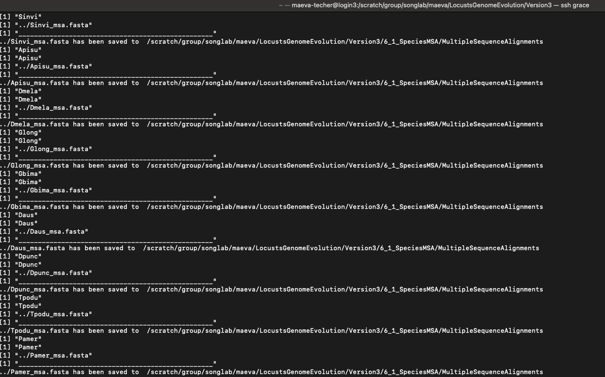
./scripts/DataMSA.R ./scripts/inputurls_13polyneoptera_May2025.txt /scratch/group/songlab/maeva/LocustsGenomeEvolution/Polyneoptera_FINAL/5_OrthoFinder/fasta/Results_May26_iqtree/MultipleSequenceAlignments/This is the final messages we get when it is successful.
Once we have obtained all the files, we go to the next step which is
filtering the protein alignment files to contain only the subset of
genes that will be called by PAL2NAL. This is due to the
fact that certain genes were not classified in orthogroups.
ml GCC/13.2.0  OpenMPI/4.1.6 R_tamu/4.4.1
export R_LIBS=$SCRATCH/R_LIBS_USER/

# Example for Schistocerca only
./scripts/FilteringCDSbyMSA.R ./scripts/inputurls_Schistocerca_Jan2025.txt

# Example for Polyneoptera
./scripts/FilteringCDSbyMSA.R ./scripts/inputurls_13polyneoptera_May2025.txt
Some of the files seems to have discrepancy of one “>” entry line
between the protein and cds file (due to a concatenation error that I
could not troubleshoot) so we are going to run the script
doublecheckCDSbyMAS which I created to remove extra
line.
# Example for Schistocerca only
./scripts/doublecheckCDSbyMAS ./scripts/inputurls_Schistocerca_Jan2025.txt

# Example for Polyneoptera
./scripts/doublecheckCDSbyMAS ./scripts/inputurls_13polyneoptera_May2025.txt

# You can also check if there is a difference with the following quick steps
grep ">" ./6_1_SpeciesMSA/proteins_Sscub.fasta | sort > proteins_Sscub_names.txt
grep ">" ./6_2_FilteredCDS/filtered_Sscub_cds.fasta | sort > cds_Sscub_names.txt
diff proteins_Sscub_names.txt cds_Sscub_names.txt
The following is the content of doublecheckCDSbyMAS:
#!/bin/bash

# Check if input file is provided
if [ "$#" -lt 1 ]; then
  echo "Usage: $0 <input_file>"
  exit 1
fi

# Input file containing species information
input_file=$1

# Directories
protein_dir="./6_1_SpeciesMSA"
cds_dir="./6_2_FilteredCDS"
backup_dir="$protein_dir/backup"
log_file="./cleaning_check.log"

# Create necessary directories
mkdir -p "$backup_dir"
rm -f "$log_file"  # Clear previous logs

# Extract species abbreviations (no header in the file)
species_list=$(awk -F',' '{print $4}' "$input_file")

# Loop through each species
for species in $species_list; do
  protein_file="$protein_dir/proteins_${species}.fasta"
  cds_file="$cds_dir/filtered_${species}_cds.fasta"
  cleaned_protein_file="$protein_dir/proteins_${species}_cleaned.fasta"
  cleaned_cds_file="$cds_dir/filtered_${species}_cds_cleaned.fasta"

  echo "Processing species: $species"

  # Check if protein and CDS files exist
  if [[ -f "$protein_file" && -f "$cds_file" ]]; then
    # Backup the original protein file
    cp "$protein_file" "$backup_dir/proteins_${species}.fasta.bak"
    echo "Backup created for: $protein_file -> $backup_dir/proteins_${species}.fasta.bak"

    # Cleaning Step: Align sequence headers between protein and CDS files
    grep ">" "$protein_file" | sort > proteins_names.txt
    grep ">" "$cds_file" | sort > cds_names.txt

    # Identify common sequence headers
    comm -12 proteins_names.txt cds_names.txt > common_names.txt

    # Check if common_names.txt is empty (indicating no matching headers)
    if [[ ! -s common_names.txt ]]; then
      echo "ERROR: No common sequence headers found for species: $species" >> "$log_file"
      echo "ERROR: Cleaning failed for species: $species due to no matching sequence headers."
      continue
    fi

    # Filter protein file
    grep -A 1 -Ff common_names.txt "$protein_file" > "$cleaned_protein_file" || {
      echo "ERROR: Failed to clean protein file for species: $species" >> "$log_file"
      continue
    }

    # Filter CDS file
    grep -A 1 -Ff common_names.txt "$cds_file" > "$cleaned_cds_file" || {
      echo "ERROR: Failed to clean CDS file for species: $species" >> "$log_file"
      continue
    }

    # Replace the original files with cleaned versions
    mv "$cleaned_protein_file" "$protein_file"
    mv "$cleaned_cds_file" "$cds_file"

    # Perform grep check to validate cleaning
    grep ">" "$protein_file" | sort > proteins_names_cleaned.txt
    grep ">" "$cds_file" | sort > cds_names_cleaned.txt
    diff_output=$(diff proteins_names_cleaned.txt cds_names_cleaned.txt)

    if [[ -z "$diff_output" ]]; then
      echo "Check passed for species: $species" >> "$log_file"
      echo "Protein and CDS sequence names match for species: $species."
    else
      echo "Check failed for species: $species" >> "$log_file"
      echo "Protein and CDS sequence names mismatch for species: $species." >> "$log_file"
      echo "$diff_output" >> "$log_file"
    fi

  else
    echo "ERROR: Missing files for species: $species" >> "$log_file"
    echo "ERROR: Protein or CDS file missing for species: $species. Skipping."
  fi
done

# Cleanup temporary files
rm -f proteins_names.txt cds_names.txt common_names.txt proteins_names_cleaned.txt cds_names_cleaned.txt

echo "All species processed. Logs saved to $log_file."
2. Generating codon-aware nucleotide alignments
PAL2NAL is installed on Grace as a module but the same
version is available in the script of this repository. We will use the
inputs generated in the previous step to obtain codon-aware
alignments.
# Example for Schistocerca only
./scripts/DataRunPAL2NAL ./scripts/inputurls_Schistocerca_Jan2025.txt

# Example for Polyneoptera
./scripts/DataRunPAL2NAL ./scripts/inputurls_13polyneoptera_May2025.txt
3. Assembling nucleotide sequence orthogroups for input in HyPHY
From M. Bardull: For some models like BUSTED, we need files that
contain orthologous nucleotide sequences from each species. Therefore,
we must recombine our codon-aware alignments in a step that is the
inverse of previous steps. To do this, use the R script
./scripts/DataSubsetCDS.R. Run with the command:
ml GCC/13.2.0  OpenMPI/4.1.6 R_tamu/4.4.1
export R_LIBS=$SCRATCH/R_LIBS_USER/

# Example for Schistocerca only
./scripts/DataSubsetCDS.R ./scripts/inputurls_Schistocerca_Jan2025.txt /scratch/group/songlab/maeva/LocustsGenomeEvolution/Schistocerca_I2/5_OrthoFinder/fasta/Results_Jan15_I2/MultipleSequenceAlignments/

# Example for Polyneoptera
 ./scripts/DataSubsetCDS.R ./scripts/inputurls_13polyneoptera_May2025.txt /scratch/group/songlab/maeva/LocustsGenomeEvolution/Polyneoptera_FINAL/5_OrthoFinder/fasta/Results_May26_iqtree/MultipleSequenceAlignments/
From M. Bardull: BUSTED will not run on sequences which contain stop
codons, even if these are reasonable, terminal stop codons.
HypPhy includes a utility which will mask these these
terminal stop codons in the orthogroups (there should be few-to-no other
stop codons, because our alignments are codon-aware). To execute this
step, use the following:
module purge
ml GCC/13.3.0  OpenMPI/5.0.3 HyPhy/2.5.71

./scripts/DataRemoveStopCodons

# for large groups launch it with sbatch
sbatch ./scripts/DataRemoveStopCodons
4. Preparing labeled phylogenies
Before performing a signature of selection analysis using HyPhy, it is important to note that some methods such as RELAX, require the phylogeny to have labeled branches to define branches. These labels define branch sets for selection testing and allow to compare selection pressures.
So we modify the script LabellingPhylogeniesHYPHY.R
ml GCC/13.2.0 OpenMPI/4.1.6 R_tamu/4.4.1
export R_LIBS=$SCRATCH/R_LIBS_USER/
# Example for Schistocerca only
./scripts/LabellingPhylogeniesHYPHY.R /scratch/group/songlab/maeva/LocustsGenomeEvolution/Schistocerca_I2/5_OrthoFinder/fasta/Results_Jan15_I2/Resolved_Gene_Trees/ Locusts.txt Locusts
# Example for Polyneoptera
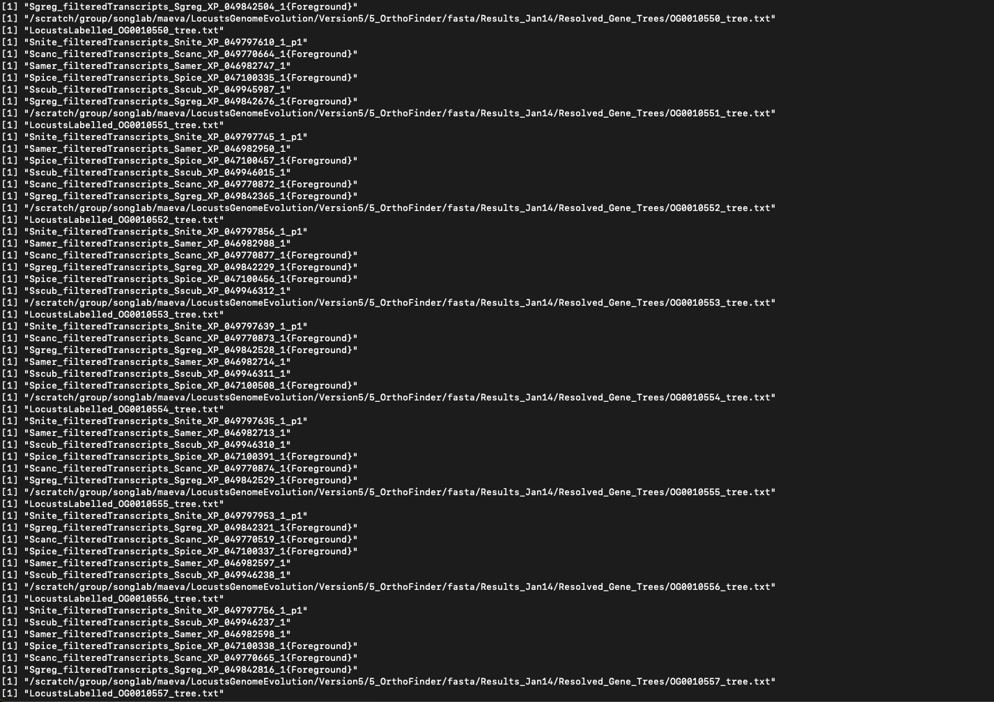
./scripts/LabellingPhylogeniesHYPHY.R /scratch/group/songlab/maeva/LocustsGenomeEvolution/Polyneoptera_FINAL/5_OrthoFinder/fasta/Results_May26_iqtree/Resolved_Gene_Trees/ Locusts.txt LocustsHow it appears when it is successful. You can see that the locust species are labelled with {Foreground}.
After running BUSTED one time, I realized that I want to check the
signal of selection only on Schistocerca and Locusta.
For that, I am pruning the trees and the fasta files of Polyneoptera if
I want to keep it with the following script
PruningLabellingPhylogeniesHYPHY.R:
ml GCC/13.2.0  OpenMPI/4.1.6 R_tamu/4.4.1
export R_LIBS=$SCRATCH/R_LIBS_USER/

  # Example for Polyneoptera
./scripts/PruningLabellingPhylogeniesHYPHY.R /scratch/group/songlab/maeva/LocustsGenomeEvolution/Polyneoptera_FINAL/5_OrthoFinder/fasta/Results_May26_iqtree/Resolved_Gene_Trees/ Locusts.txt Species2keep.txt Locusts
How the input files should look:
[maeva-techer@grace1 Polyneoptera_FINAL]$ cat Species2keep.txt
Samer
Sscub
Snite
Sgreg
Scanc
Spice
Lmigr
Details of the PruningLabellingPhylogeniesHYPHY.R are
pasted below. If we used these folders, we will have to modify our
Run{HYPHYMETHOD} to reflect the source of the new fasta sequences in
8_2_RemovedStops_Pruned:
[maeva-techer@grace1 Polyneoptera_FINAL]$ cat scripts/PruningLabellingPhylogeniesHYPHY.R
#!/usr/bin/env Rscript

# ============================= #
#        LOAD LIBRARIES        #
# ============================= #
suppressPackageStartupMessages({
  library(fs)
  library(Biostrings)
  library(ape)
  library(tidyverse)
  library(purrr)
})

# ============================= #
#         READ ARGUMENTS       #
# ============================= #
args <- commandArgs(trailingOnly = TRUE)
if (length(args) < 3) {
  stop("Usage: Rscript LabelAndPruneTreesHYPHY.R <tree_dir> <foreground_species.txt> <retained_species.txt>", call. = FALSE)
}

tree_dir <- args[1]
fg_species_file <- args[2]
retained_species_file <- args[3]
output_prefix <- ifelse(length(args) >= 4, args[4], "labelled")

# ============================= #
#       READ SPECIES FILES     #
# ============================= #
foreground_species <- read_lines(fg_species_file) %>% str_trim()
retained_species <- read_lines(retained_species_file) %>% str_trim()

# ============================= #
#         OUTPUT SETUP         #
# ============================= #
tree_output_dir <- file.path("9_1_LabelledPhylogenies_Pruned", output_prefix)
fasta_input_dir <- "8_2_RemovedStops"
fasta_output_dir <- "8_2_RemovedStops_Pruned"

dir_create(tree_output_dir)
dir_create(fasta_output_dir)

# ============================= #
#       LABEL + PRUNE FUNC     #
# ============================= #
multiTreeLabelAndPrune <- function(tree_path, retained_sp, foreground_sp, export_path) {
  tree <- read.tree(tree_path)

  message("🌳 Processing tree: ", basename(tree_path))

  # Get tip abbreviations
  tip_species <- sapply(strsplit(tree$tip.label, "_"), `[`, 1)
  keep_tips <- tree$tip.label[tip_species %in% retained_sp]

  if (length(keep_tips) < 4) {
    message("⚠️ Skipping ", basename(tree_path), " — fewer than 4 retained tips.")
    return(NULL)
  }

  pruned_tree <- drop.tip(tree, setdiff(tree$tip.label, keep_tips))

  # Label foreground tips
  pruned_tree$tip.label <- map_chr(pruned_tree$tip.label, function(label) {
    sp_abbr <- strsplit(label, "_")[[1]][1]
    if (sp_abbr %in% foreground_sp) paste0(label, "{Foreground}") else label
  })

  # Label nodes leading to foreground
  fg_tips <- grep("\\{Foreground\\}", pruned_tree$tip.label)
  if (length(fg_tips) > 0) {
    pruned_tree$node.label <- rep("", pruned_tree$Nnode)
    ancestor_nodes <- pruned_tree$edge[pruned_tree$edge[, 2] %in% fg_tips, 1]
    pruned_tree$node.label[ancestor_nodes - length(pruned_tree$tip.label)] <- "{Foreground}"
  }

  write.tree(pruned_tree, file = export_path)
  message("✅ Tree saved to: ", export_path)
}

# ============================= #
#       FASTA PRUNE FUNC       #
# ============================= #
pruneFastaBySpecies <- function(fasta_path, retained_sp, export_path) {
  message("🧬 Processing FASTA: ", basename(fasta_path))
  fasta <- readDNAStringSet(fasta_path)

  keep_idx <- vapply(names(fasta), function(x) {
    sp_abbr <- strsplit(x, "_")[[1]][1]
    sp_abbr %in% retained_sp
  }, logical(1))

  pruned_fasta <- fasta[keep_idx]
  if (length(pruned_fasta) == 0) {
    message("⚠️ No retained sequences in: ", basename(fasta_path))
    return(NULL)
  }

  writeXStringSet(pruned_fasta, filepath = export_path)
  message("✅ FASTA saved to: ", export_path)
}


# ============================= #
#         MAIN LOOP            #
# ============================= #
# Prune + label trees
tree_files <- dir_ls(tree_dir, regexp = "\\.txt$|\\.treefile$|\\.nwk$")
walk(tree_files, function(tree_file) {
  og_name <- path_file(tree_file)
  export_name <- file.path(tree_output_dir, paste0(output_prefix, "Labelled_", og_name))
  multiTreeLabelAndPrune(tree_file, retained_species, foreground_species, export_name)
})

# Prune FASTA files
fasta_files <- dir_ls(fasta_input_dir, glob = "*.fasta")
walk(fasta_files, function(fa_file) {
  out_fa <- file.path(fasta_output_dir, path_file(fa_file))
  pruneFastaBySpecies(fa_file, retained_species, out_fa)
})

message("🎉 All trees and FASTA files processed and saved.")
5. Annotating proteins with InterProScan and Orthogroups with KinFin
As part of the process, we want to make sure that the genes under selection have meaningful biological interpretations through functional annotation and GO enrichment analysis. To achieve this, we will use InterProScan to annotate individual genes and KinFin to generate gene-level annotations, assigning functional categories to entire orthogroups. This approach aligns with the orthogroup-level focus of our analyses in aBSREL, BUSTED, and RELAX, providing insights into the functional relevance of selective pressures.
For that we run the following command:
# Example for Schistocerca only
./scripts/RunningInterProScan_modif ./scripts/inputurls_Schistocerca_Jan2025.txt /scratch/group/songlab/maeva/LocustsGenomeEvolution/Schistocerca_I2/5_OrthoFinder/fasta/

# Example for Polyneoptera
./scripts/RunningInterProScan_modif ./scripts/inputurls_13polyneoptera_Jan2025.txt /scratch/group/songlab/maeva/LocustsGenomeEvolution/Polyneoptera_I2/5_OrthoFinder/fasta/

# we replace the version of interproscan to the most recent: interproscan-5.72-103.0

# we also comment out ax.set_facecolor('white')' on lines 681 and 1754 of ./kinfin/src/kinfin.py
Here is the details of
./scripts/RunningInterProScan_modif
#!/bin/bash

## SLURM Job Specifications
#SBATCH --job-name=interproscan         # Set the job name
#SBATCH --time=4-00:00:00              # Set the wall clock limit to 4 days
#SBATCH --ntasks=1                     # Request 1 task
#SBATCH --cpus-per-task=12             # Request 12 CPUs for the task
#SBATCH --mem=100G                     # Request 100GB memory
#SBATCH --output=interproscan_%j.out   # Standard output log
#SBATCH --error=interproscan_%j.err    # Standard error log

# Ensure the script receives correct arguments
if [ "$#" -ne 2 ]; then
  echo "Usage: $0 <input_file> <path_to_proteins_directory>"
  exit 1
fi

input_file=$1
proteins_dir=$2

# Load necessary modules
ml Java/11.0.2
ml WebProxy

export http_proxy=http://10.73.132.63:8080
export https_proxy=http://10.73.132.63:8080

# Main working directories
interpro_dir="./11_InterProScan/interproscan-5.72-103.0"
output_dir="$interpro_dir/out"
backup_dir="./11_InterProScan/backup"

# Create necessary directories
mkdir -p "$output_dir"
mkdir -p "$backup_dir"

# Iterate through the input file to process each species
while read -r line; do
  # Extract the species abbreviation
  name=$(echo "$line" | awk -F',' '{print $4}')
  protein_name="${name}_filteredTranscripts.fasta"

  echo "Processing species: $name"

  # Check if the protein file exists
  protein_path="$proteins_dir/$protein_name"
  if [ ! -f "$protein_path" ]; then
    echo "Protein file $protein_name not found in $proteins_dir. Skipping."
    continue
  fi

  # Check if the species has already been annotated
  annotated_file="$output_dir/${protein_name}.tsv"
  if [ -f "$annotated_file" ]; then
    echo "$annotated_file exists; skipping $name."
    continue
  fi

  # Backup original protein file and clean it
  cp "$protein_path" "$backup_dir/${protein_name}.bak"
  cp "$protein_path" "$interpro_dir/$protein_name"
  sed -i'.original' -e "s|\*||g" "$interpro_dir/$protein_name"
  rm "$interpro_dir/${protein_name}.original"

  # Run InterProScan
  echo "Running InterProScan for $protein_name..."
  cd "$interpro_dir"
  ./interproscan.sh -i "$protein_name" -d out/ -t p --goterms -appl Pfam -f TSV
  cd - > /dev/null

done < "$input_file"

# Combine all annotated results into a single file
cat "$output_dir"/*.tsv > "$interpro_dir/all_proteins.tsv"
echo "Annotation completed. Combined results stored in $interpro_dir/all_proteins.tsv."

# KinFin Preparation
kinfin_dir="./11_InterProScan/kinfin"
if [ ! -d "$kinfin_dir" ]; then
  echo "KinFin not installed. Please install KinFin and rerun this step."
  exit 1
fi

# Convert InterProScan results to KinFin-compatible format
echo "Preparing InterProScan results for KinFin..."
"$kinfin_dir/scripts/iprs2table.py" -i "$interpro_dir/all_proteins.tsv" --domain_sources Pfam

# Copy Orthofinder files to KinFin directory
cp 5_OrthoFinder/fasta/OrthoFinder/Results*/Orthogroups/Orthogroups.txt "$kinfin_dir/"
cp 5_OrthoFinder/fasta/OrthoFinder/Results*/WorkingDirectory/SequenceIDs.txt "$kinfin_dir/"
cp 5_OrthoFinder/fasta/OrthoFinder/Results*/WorkingDirectory/SpeciesIDs.txt "$kinfin_dir/"

# Create KinFin configuration file
echo '#IDX,TAXON' > "$kinfin_dir/config.txt"
sed 's/: /,/g' "$kinfin_dir/SpeciesIDs.txt" | cut -f 1 -d"." >> "$kinfin_dir/config.txt"

# Run KinFin functional annotation
echo "Running KinFin functional annotation..."
"$kinfin_dir/kinfin" --cluster_file "$kinfin_dir/Orthogroups.txt" \
  --config_file "$kinfin_dir/config.txt" \
  --sequence_ids_file "$kinfin_dir/SequenceIDs.txt" \
  --functional_annotation functional_annotation.txt

echo "Functional annotation completed."
6. BUSTED
We will perform BUSTED analysis using both unlabeled and labelled phylogeny.
The unlabeled gene tree phylogeny will allow for an exploratory analysis, testing all Polyneoptera for positive selection. While this approach provides a broad overview, it comes at the cost of reduced statistical power due to multiple testing.
In contrast, the labelled gene tree phylogeny will focus specifically on migratory locust species compared to all other species or to non-migratory grasshoppers, enabling us to associate traits with selective pressures.
Note: The new version of OrthoFinder
makes a list of SingleCopy Orthologues by adding a N0:H
before the orthogroup name. N0.HOG0000086 N0.HOG0000090 N0.HOG0000212
N0.HOG0000220 N0.HOG0000478 N0.HOG0000479 N0.HOG0000503
N0.HOG0000505
So we need to clean that up before running our files using the command
sed 's/^N0\.HOG/OG/' Orthogroups_SingleCopyOrthologues.txt > Orthogroups_SingleCopyOrthologues_renamed.txtRunning the analysis
We will perform BUSTED analysis using both unlabeled and labelled gene tree phylogeny. The unlabeled phylogeny will allow for a gene-wide exploratory analysis treating the entire tree of Polyneoptera as foreground.
# For unlabelled phylogeny
sbatch scripts/RunBUSTED_May2025.sh \
/scratch/group/songlab/maeva/LocustsGenomeEvolution/Schistocerca_I2/5_OrthoFinder/fasta/Results_Jan15_I2/Resolved_Gene_Trees \
/scratch/group/songlab/maeva/LocustsGenomeEvolution/Schistocerca_I2/5_OrthoFinder/fasta/Results_Jan15_I2/Orthogroups/Orthogroups_SingleCopyOrthologues.txt

# For labelled phylogeny
sbatch ./scripts/RunBUSTED_labeled_May2025.sh \
/scratch/group/songlab/maeva/LocustsGenomeEvolution/Schistocerca_I2/9_1_LabelledPhylogenies/Locusts \
Locusts \
/scratch/group/songlab/maeva/LocustsGenomeEvolution/Schistocerca_I2/5_OrthoFinder/fasta/Results_Jan15_I2/Orthogroups/Orthogroups_SingleCopyOrthologues.txt

################################
# Polyneoptera
# For unlabelled phylogeny
sbatch scripts/RunBUSTED_May2025.sh  \
/scratch/group/songlab/maeva/LocustsGenomeEvolution/Polyneoptera_FINAL/5_OrthoFinder/fasta/Results_May26_iqtree/Resolved_Gene_Trees/ \
/scratch/group/songlab/maeva/LocustsGenomeEvolution/Polyneoptera_FINAL/5_OrthoFinder/fasta/Results_May26_iqtree/Orthogroups/Orthogroups_SingleCopyOrthologues_selanalysiswide.txt

# For labelled phylogeny
sbatch ./scripts/RunBUSTED_labeled_May2025.sh \
/scratch/group/songlab/maeva/LocustsGenomeEvolution/Polyneoptera_FINAL/9_1_LabelledPhylogenies/Locusts \
Locusts \
/scratch/group/songlab/maeva/LocustsGenomeEvolution/Polyneoptera_FINAL/5_OrthoFinder/fasta/Results_May26_iqtree/Orthogroups/Orthogroups_SingleCopyOrthologues_selanalysiswide.txt

# For labelled phylogeny PRUNED
sbatch ./scripts/RunBUSTED_labeled_June2025.sh \
/scratch/group/songlab/maeva/LocustsGenomeEvolution/Polyneoptera_FINAL/9_1_LabelledPhylogenies_Pruned/Locusts \
Locusts \
/scratch/group/songlab/maeva/LocustsGenomeEvolution/Polyneoptera_FINAL/5_OrthoFinder/fasta/Results_May26_iqtree/Orthogroups/Orthogroups_SingleCopyOrthologues_selanalysiswide.txt
If we want to run R interactively on the cluster:
srun --ntasks 1 --cpus-per-task 16 --mem 50G --time 05:00:00 --pty bash
ml GCC/13.2.0  OpenMPI/4.1.6 R_tamu/4.4.1
ml WebProxy
export R_LIBS=$SCRATCH/R_LIBS_USER/

Rscript ./scripts/Parsing_BUSTEDresulsr_unlabel.R
Parsing the json files
To parse all the details from the BUSTED by testing all branches to
see if we have selection pressures
./scripts/Parsing_BUSTEDresulsr_unlabel_June2025.R:
#!/usr/bin/env Rscript

library(jsonlite)
library(tidyverse)
library(hexbin)

# ============ SETTINGS ============
input_dir <- "/scratch/group/songlab/maeva/LocustsGenomeEvolution/Polyneoptera_FINAL/8_3_BustedResults"
single_copy_file <- "/scratch/group/songlab/maeva/LocustsGenomeEvolution/Polyneoptera_FINAL/5_OrthoFinder/fasta/Results_May26_iqtree/Orthogroups/Orthogroups_SingleCopyOrthologues_selanalysiswide.txt"
output_dir <- "/scratch/group/songlab/maeva/LocustsGenomeEvolution/Polyneoptera_FINAL/ParsedBUSTEDResults_unlabeled"
dir.create(output_dir, showWarnings = FALSE, recursive = TRUE)

# ============ JSON PARSER ============
parse_busted <- function(file) {
  tryCatch({
    busted <- jsonlite::fromJSON(file)

    og <- stringr::str_extract(basename(file), "^OG[0-9]+")
    busted_input_file <- busted[["input"]][["file name"]]
    busted_pval <- as.numeric(busted[["test results"]][["p-value"]])

    # Corrected metadata fields
    aln_length <- busted[["input"]][["number of sites"]]
    seq_count  <- busted[["input"]][["number of sequences"]]

    # Rate model info: safely extract from 'Test'
    rate_info <- busted[["fits"]][["Unconstrained model"]][["Rate Distributions"]][["Test"]]

    omega_vals <- sapply(rate_info, function(x) as.numeric(x[["omega"]]))
    prop_vals  <- sapply(rate_info, function(x) as.numeric(x[["proportion"]]))

    # Optional: if missing, use NA
    omega3 <- ifelse(length(omega_vals) >= 3, omega_vals[3], NA)
    prop3  <- ifelse(length(prop_vals) >= 3, prop_vals[3], NA)

    # Flag potential overfitting
    suspect <- is.na(omega3) || omega3 > 1000 || prop3 < 0.001 || aln_length < 100 || seq_count < 4

    tibble::tibble(
      file = file,
      input_file = busted_input_file,
      orthogroup = og,
      seq_count = seq_count,
      aln_length = aln_length,
      omega1 = omega_vals[1],
      prop1  = prop_vals[1],
      omega2 = omega_vals[2],
      prop2  = prop_vals[2],
      omega3 = omega3,
      prop_sites = prop3,
      pval = busted_pval,
      padj = p.adjust(busted_pval, method = "BH"),
      significant = p.adjust(busted_pval, method = "BH") < 0.05,
      suspect_result = suspect
    )
  }, error = function(e) {
    message("⚠️ Error parsing: ", file, " -> ", e$message)
    return(NULL)
  })
}


# ============ Parse All JSON Files ============
json_files <- list.files(input_dir, pattern = "\\.json$", full.names = TRUE)
parsed <- map_dfr(json_files, parse_busted)

# ============ Save All Results ============
write_csv(parsed, file.path(output_dir, "BUSTED_results_all.csv"))
write_csv(filter(parsed, significant), file.path(output_dir, "BUSTED_results_significant.csv"))

# ============ Optional: Filter for Single-Copy Orthogroups ============
if (file.exists(single_copy_file)) {
  sc_ogs <- read_lines(single_copy_file) %>% str_trim()
  parsed_sc <- parsed %>% filter(orthogroup %in% sc_ogs)

  write_csv(parsed_sc, file.path(output_dir, "BUSTED_results_singlecopy.csv"))
  write_csv(filter(parsed_sc, significant), file.path(output_dir, "BUSTED_results_singlecopy_significant.csv"))
}

# ============ Quick Summary ============
message("✅ Parsed: ", nrow(parsed), " orthogroups")
message("🧬 Positive selection (FDR < 0.05): ", sum(parsed$significant))


library(ggplot2)

# Create hexbin plot for significant results
p <- ggplot(filter(parsed, significant), aes(x = prop_sites, y = omega3)) +
  geom_hex(bins = 40) +
  scale_fill_gradient(trans = "log10", low = "#ccf0ed", high = "#014a44") +
  scale_x_log10() +
  scale_y_log10() +
  labs(
    title = "Selection Landscape for Positively Selected Genes",
    x = "Proportion of Sites Under Selection (log10)",
    y = "Strength of Selection (omega, log10)",
    fill = "Number of Genes"
  ) +
  theme_bw()

ggsave(filename = file.path(output_dir, "busted_hexbin_plot.pdf"), plot = p, width = 7, height = 6)

p2 <- ggplot(parsed, aes(x = omega3, y = -log10(padj), color = significant)) +
  geom_point(alpha = 0.8) +
  scale_color_manual(values = c("FALSE" = "grey60", "TRUE" = "red")) +
  labs(
    x = "Strength of Selection (omega3)",
    y = expression(-log[10]~"(FDR-adjusted p-value)"),
    color = "Significant"
  ) +
  theme_minimal()

ggsave(file.path(output_dir, "busted_volcano_plot.pdf"), p2, width = 7, height = 6)

p3 <- parsed %>%
  filter(significant) %>%
  arrange(padj) %>%
  slice_head(n = 20) %>%
  ggplot(aes(x = reorder(orthogroup, -padj), y = -log10(padj))) +
  geom_col(fill = "steelblue") +
  coord_flip() +
  labs(
    x = "Orthogroup",
    y = expression(-log[10]~"(FDR-adjusted p-value)"),
    title = "Top 20 Positively Selected Orthogroups"
  ) +
  theme_classic()

ggsave(file.path(output_dir, "busted_top20_barplot.pdf"), p3, width = 8, height = 6)
To parse the results from the *json files from the BUSTED-PH with
migratory locusts as foreground branches we run this
./scripts/Parsing_BUSTEDresulsr_labelled_June2025.R:
#!/usr/bin/env Rscript

# ============================= #
#         LOAD LIBRARIES       #
# ============================= #
suppressPackageStartupMessages({
  library(tidyverse)
  library(jsonlite)
  library(fs)
  library(ggplot2)
  library(patchwork)
})


# ============================= #
#      PARSING UTILITIES       #
# ============================= #
loadJsons <- function(dir) {
  files <- fs::dir_ls(dir, glob = "*.json")
  purrr::map(files, jsonlite::read_json)
}

.getTested <- function(file, json) {
  tibble(file = file, id = names(json), condition = unlist(json))
}

.getTestResultsBPH <- function(file, json) {
  tibble(
    file = file,
    test = c("test results", "test results background", "test results shared distribution"),
    lrt = c(json$`test results`$LRT,
            json$`test results background`$LRT,
            json$`test results shared distributions`$LRT),
    pval = c(json$`test results`$`p-value`,
             json$`test results background`$`p-value`,
             json$`test results shared distributions`$`p-value`)
  )
}

.getBranchAttributesBPH <- function(file, json) {
  partitions <- json[-length(json)]
  map_dfr(partitions, function(pt) {
    imap_dfr(pt, ~{
      values_clean <- suppressWarnings(as.numeric(unlist(.x)))
      if (length(values_clean) == 0 || length(values_clean) != length(.x)) return(NULL)
      tibble(file = file, id = .y, models = names(.x), values = values_clean)
    })
  })
}

parseBustedPh <- function(jsons, dataset_label) {
  test.results <- list()
  grouping <- list()
  branch.attributes <- list()

  for (i in seq_along(jsons)) {
    js <- jsons[[i]]
    file.name <- sub(".fasta", "", basename(js$input$`file name`))
    test.results[[i]] <- .getTestResultsBPH(file.name, js)
    grouping[[i]] <- .getTested(file.name, js$tested$`0`)
    branch.attributes[[i]] <- .getBranchAttributesBPH(file.name, js$`branch attributes`)
  }

  list(
    `test results` = bind_rows(test.results) %>% mutate(dataset = dataset_label),
    grouping = bind_rows(grouping) %>% mutate(dataset = dataset_label),
    branch_attributes = bind_rows(branch.attributes)
  )
}


pcorrBUSTEDPH <- function(df, p = 0.05, corrMethod = 'fdr') {
  df %>%
    group_by(file, dataset, test) %>%
    summarise(pval = min(pval, na.rm = TRUE), .groups = "drop") %>%
    pivot_wider(names_from = test, values_from = pval) %>%
    mutate(
      adj_test = p.adjust(`test results`, method = corrMethod),
      adj_background = p.adjust(`test results background`, method = corrMethod),
      adj_dist = p.adjust(`test results shared distribution`, method = corrMethod),
      result = case_when(
        adj_test < p & adj_dist < p & adj_background > p ~ 'Selection in test branches only',
        adj_test < p & adj_background < p & adj_dist < p ~ 'Selection in both test and background, distinct regimes',
        adj_test < p & adj_background < p & adj_dist > p ~ 'Selection in both, same regime',
        adj_test > p & adj_background < p ~ 'Only background selection',
        TRUE ~ 'No significant signal'
      )
    )
}

# ============================= #
#         MAIN SCRIPT           #
# ============================= #
# Paths
fg_dir <- "/scratch/group/songlab/maeva/LocustsGenomeEvolution/Polyneoptera_FINAL/8_4_BustedResults_labeled_Pruned/Locusts/foreground/"
bg_dir <- "/scratch/group/songlab/maeva/LocustsGenomeEvolution/Polyneoptera_FINAL/8_4_BustedResults_labeled_Pruned/Locusts/background/"
out_dir <- "/scratch/group/songlab/maeva/LocustsGenomeEvolution/Polyneoptera_FINAL/ParsedBUSTEDPHResults_labeled_Pruned"
pdf_out <- file.path(out_dir, "BUSTEDPH_summary_plots.pdf")

# Load and parse
json_fg <- loadJsons(fg_dir)
json_bg <- loadJsons(bg_dir)

parsed_fg <- parseBustedPh(json_fg, "foreground")
parsed_bg <- parseBustedPh(json_bg, "background")

grouping_all <- bind_rows(parsed_fg$grouping, parsed_bg$grouping)
branch_attr_all <- bind_rows(parsed_fg$branch_attributes, parsed_bg$branch_attributes)
test_results_all <- bind_rows(parsed_fg$`test results`, parsed_bg$`test results`)
corrected <- pcorrBUSTEDPH(test_results_all)

# Save data
dir.create(out_dir, showWarnings = FALSE)
write_csv(grouping_all, file.path(out_dir, "grouping_all.csv"))
write_csv(branch_attr_all, file.path(out_dir, "branch_attributes_all.csv"))
write_csv(test_results_all, file.path(out_dir, "test_results_all.csv"))
write_csv(corrected, file.path(out_dir, "BUSTEDPH_results_corrected.csv"))

message("✅ BUSTED-PH parsed.")

# ============================= #
#     BUILD PLOT DATAFRAMES     #
# ============================= #
# Omega values
omega_df <- branch_attr_all %>%
  filter(str_detect(models, "omega")) %>%
  separate(models, into = c("rate", "category"), sep = "\\.") %>%
  pivot_wider(names_from = dataset, values_from = values) %>%
  rename(omega_category = rate)

# Merge with grouping
merged_omega <- omega_df %>%
  left_join(grouping_all, by = c("file", "id")) %>%
  filter(!is.na(foreground) & !is.na(background))

# Plot A: omega scatter
plot_a <- ggplot(merged_omega, aes(x = log10(foreground), y = log10(background))) +
  geom_point(aes(color = omega_category), alpha = 0.6, size = 1.5) +
  geom_density2d(color = "grey60", size = 0.3) +
  labs(
    x = expression(log[10]*omega[Test]),
    y = expression(log[10]*omega[Background]),
    title = "A) ω rate scatter for shared branches"
  ) +
  theme_minimal() +
  theme(legend.position = "bottom")

# Plot B: proportions and omega by rate category
proportion_df <- branch_attr_all %>%
  filter(str_detect(models, "proportion")) %>%
  separate(models, into = c("rate", "category"), sep = "\\.") %>%
  pivot_wider(names_from = dataset, values_from = values) %>%
  rename(rate_category = rate)

omega_vals_df <- branch_attr_all %>%
  filter(str_detect(models, "omega")) %>%
  separate(models, into = c("rate", "category"), sep = "\\.") %>%
  pivot_wider(names_from = dataset, values_from = values) %>%
  rename(rate_category = rate)

merged_cat <- proportion_df %>%
  left_join(omega_vals_df, by = c("file", "id", "rate_category")) %>%
  pivot_longer(cols = starts_with("foreground") | starts_with("background"),
               names_to = c("dataset", ".value"),
               names_pattern = "(foreground|background)_(.*)")

# Plot B1: Proportion
plot_b1 <- ggplot(merged_cat, aes(x = rate_category, y = proportion, fill = dataset)) +
  geom_boxplot(outlier.shape = NA, position = position_dodge(0.8)) +
  scale_y_log10() +
  labs(title = "B1) % of sites by ω-rate-category", y = "Proportion (%)", x = "ω-rate-category") +
  theme_minimal()

# Plot B2: Omega
plot_b2 <- ggplot(merged_cat, aes(x = rate_category, y = omega, fill = dataset)) +
  geom_boxplot(outlier.shape = NA, position = position_dodge(0.8)) +
  scale_y_log10() +
  labs(title = "B2) ω values by category", y = expression(omega), x = "ω-rate-category") +
  theme_minimal()

# ============================= #
#         EXPORT TO PDF         #
# ============================= #
pdf(pdf_out, width = 11, height = 8)
print(plot_a)
print(plot_b1)
print(plot_b2)
dev.off()

message("📄 Exported to: ", pdf_out)
Extracting the selected genes
We run BUSTED analysis on a total of 5,347 single copy
orthogroups for which:
- 3,094 orthogroups with 1:1 orthologs for all species
(SelecAnalysisStrict = Included). - 763 orthogroups with 1:1 orthologs
for Caelifera species (SelAnalysisLocusts = Included). - 1,490
orthogroups with mixed 1:1 orthologs with all Caelifera species
(SelAnalysisMixed = Included).
We will show the results by category.
library(ggplot2)
library(dplyr)
library(readr)
library(ggnewscale)

ortho_dir <- "/Users/maevatecher/Documents/GitHub/locust-comparative-genomics/data/orthofinder/Polyneoptera"
input_file <- file.path(ortho_dir, "Results_I2_iqtree/Orthogroups/Orthogroups_CladeAssignment_WithCopyStatus_cleaned.csv")
orthologtable <- read.csv(input_file, header = TRUE, stringsAsFactors = FALSE)

hyphy_dir <- "/Users/maevatecher/Documents/GitHub/locust-comparative-genomics/data/HYPHY_selection"
input_file2 <- file.path(hyphy_dir, "ParsedBUSTEDResults_unlabeled/BUSTED_results_all.csv")
bustedtable <- read.csv(input_file2, header = TRUE, stringsAsFactors = FALSE) %>%
  select(-input_file, -file)

busted_df <- left_join(orthologtable, bustedtable, by = c("Orthogroup" = "orthogroup"))

# Save as CSV
workDir <- "/Users/maevatecher/Documents/GitHub/locust-comparative-genomics/data"
output_file <- file.path(workDir, "HYPHY_selection/ParsedBUSTEDResults_unlabeled/busted_compiled.csv")
write.csv(busted_df, output_file, row.names = FALSE)

busted_SingleStrict <- busted_df %>%
  filter(SelAnalysisStrict == "Included")

busted_locust <- busted_df %>%
  filter(SelAnalysisLocusts == "Included")

busted_mixed <- busted_df %>%
  filter(SelAnalysisMixed == "Included")

library(dplyr)
library(tibble)

summary_table <- tibble(
  Category = c("1:1 Polyneoptera", "1:1 Caelifera only", "1:1 Mixed"),
  Total = c(
    sum(busted_df$SelAnalysisStrict == "Included", na.rm = TRUE),
    sum(busted_df$SelAnalysisLocusts == "Included", na.rm = TRUE),
    sum(busted_df$SelAnalysisMixed == "Included", na.rm = TRUE)
  ),
Significant = c(
    sum(busted_df$SelAnalysisStrict == "Included" & busted_df$padj < 0.05, na.rm = TRUE),
    sum(busted_df$SelAnalysisLocusts == "Included" & busted_df$padj < 0.05, na.rm = TRUE),
    sum(busted_df$SelAnalysisMixed == "Included" & busted_df$padj < 0.05, na.rm = TRUE)
  ),
  Suspect = c(
    sum(busted_df$SelAnalysisStrict == "Included" & busted_df$padj < 0.05 & busted_df$suspect_result == TRUE, na.rm = TRUE),
    sum(busted_df$SelAnalysisLocusts == "Included" & busted_df$padj < 0.05 & busted_df$suspect_result == TRUE, na.rm = TRUE),
    sum(busted_df$SelAnalysisMixed == "Included" & busted_df$padj < 0.05 & busted_df$suspect_result == TRUE, na.rm = TRUE)
  )
)%>%
  mutate(True_Selected = Significant - Suspect)

knitr::kable(summary_table, caption = "Summary of BUSTED results per orthogroup category")| Category | Total | Significant | Suspect | True_Selected |
|---|---|---|---|---|
| 1:1 Polyneoptera | 3094 | 1414 | 280 | 1134 |
| 1:1 Caelifera only | 763 | 210 | 59 | 151 |
| 1:1 Mixed | 1490 | 559 | 110 | 449 |
A total of 2,183 orthogroups showed signature of selection but only 1,734 showed omega3 values that were not suspect (due to model over fitting, short alignment, low divergence).
Below is the selection landscape for all orthogroups with corrected (BH) p-value < 0.05.
# Filter for significant genes
parsed <- busted_df %>%
  filter(!is.na(padj), padj < 0.05) %>%
  filter(!is.na(prop_sites), !is.na(omega3))  # <- ensure both axes are numeric

# Separate the suspect results
suspect_points <- parsed %>%
  filter(suspect_result == TRUE)

# Base: All significant data
base_data <- parsed %>% filter(suspect_result == FALSE)
suspect_data <- parsed %>% filter(suspect_result == TRUE)

p <- ggplot() +
  geom_hex(data = base_data, aes(x = prop_sites, y = omega3), bins = 40) +
  scale_fill_gradient(trans = "log10", low = "#ccf0ed", high = "#014a44") +
  new_scale_fill() +  # Needed from ggh4x or ggnewscale to add a second fill scale

  geom_hex(data = suspect_data, aes(x = prop_sites, y = omega3), bins = 40, inherit.aes = FALSE) +
  scale_fill_gradient(trans = "log10", low = "mistyrose", high = "red", name = "Suspect Count") +

  scale_x_log10() +
  scale_y_log10() +
  labs(
    title = "Selection Landscape: Suspect Results in Red Hexes",
    x = "Proportion of Sites Under Selection (log10)",
    y = "Strength of Selection (omega, log10)"
  ) +
  theme_bw()

p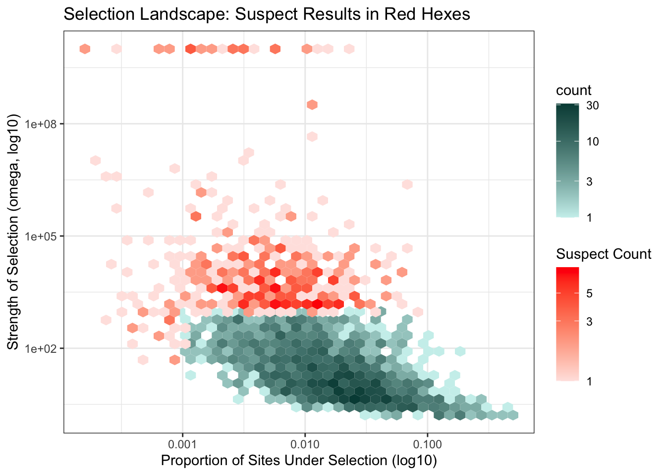
| Version | Author | Date |
|---|---|---|
| a2d2955 | Maeva TECHER | 2025-07-01 |
Below we show the hex bin graphs for only the 1:1 Polyneoptera and 1:1 Caelifera selection landscapes.
# Filter for significant genes
parsed_polyneoptera <- busted_SingleStrict %>%
  filter(!is.na(padj), padj < 0.05) %>%
  filter(!is.na(prop_sites), !is.na(omega3)) %>% # <- ensure both axes are numeric
  filter(suspect_result == FALSE)

# Plot
p <- ggplot(parsed_polyneoptera, aes(x = prop_sites, y = omega3)) +
  geom_hex(bins = 40) +
  scale_fill_gradient(trans = "log10", low = "#ccf0ed", high = "#014a44") +
  scale_x_log10() +
  scale_y_log10() +
  labs(
    title = "Selection Landscape for Positively Selected Genes (1:1 Polyneoptera)",
    x = "Proportion of Sites Under Selection (log10)",
    y = "Strength of Selection (omega, log10)",
    fill = "Number of Orthogroups"
  ) +
  theme_bw()

p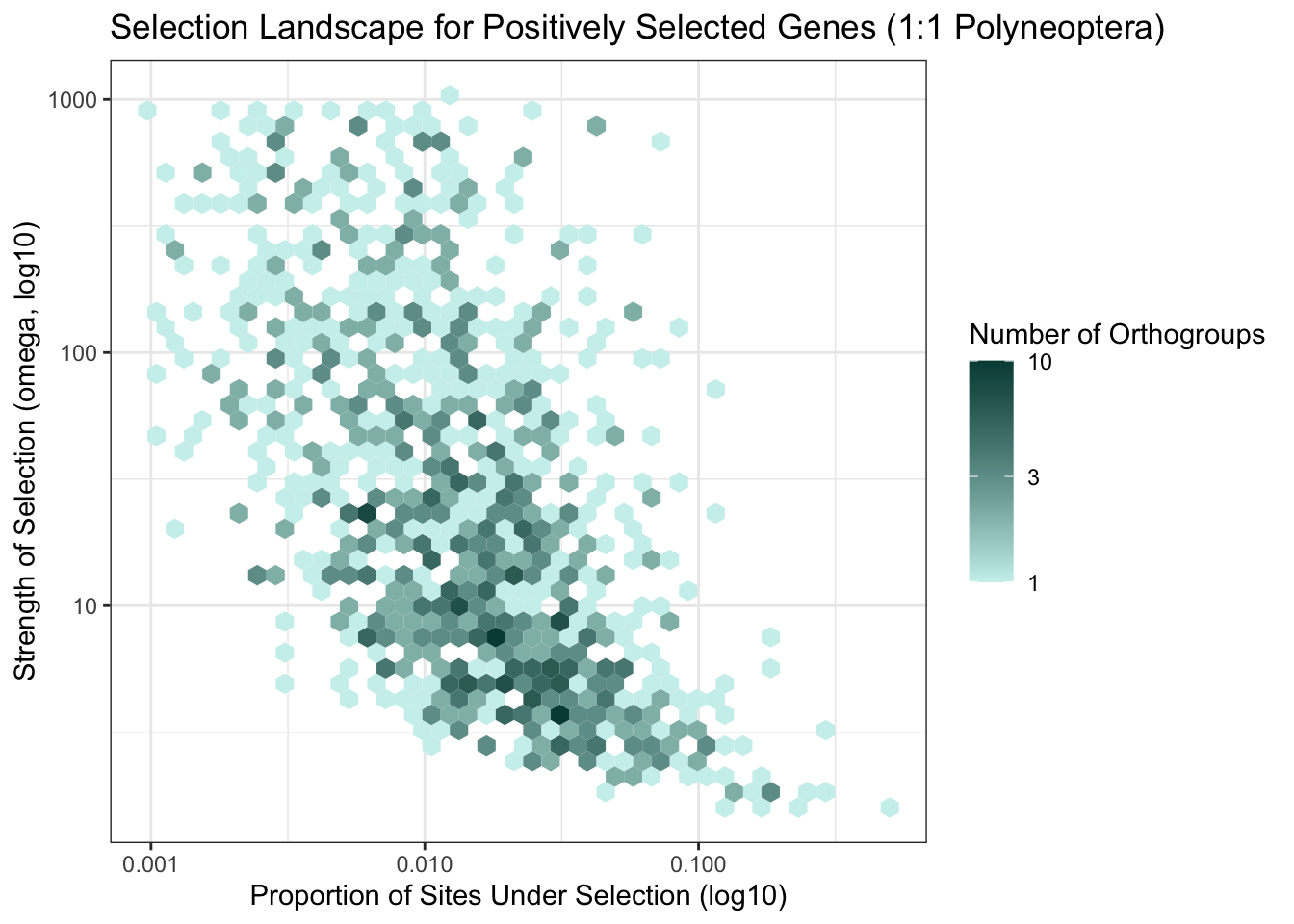
| Version | Author | Date |
|---|---|---|
| a2d2955 | Maeva TECHER | 2025-07-01 |
# Filter for significant genes
parsed_locust <- busted_locust %>%
  filter(!is.na(padj), padj < 0.05) %>%
  filter(!is.na(prop_sites), !is.na(omega3)) %>% # <- ensure both axes are numeric
  filter(suspect_result == FALSE)

# We make a hexbin graph only for genes that are locust only

ggplot(parsed_locust, aes(x = prop_sites, y = omega3)) +
  geom_hex(bins = 40) +
  scale_fill_gradient(trans = "log10", low = "#e6f2ff", high = "#084594") +
  scale_x_log10() +
  scale_y_log10() +
  labs(
    title = "Selection on Strict Single-Copy Genes (1:1 Caelifera only)",
    x = "Proportion of Sites Under Selection (log10)",
    y = "Strength of Selection (omega, log10)",
    fill = "Number of Orthogroups"
  ) +
  theme_bw()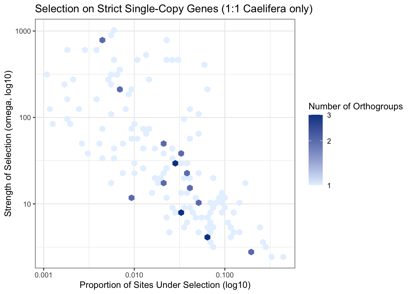
| Version | Author | Date |
|---|---|---|
| a2d2955 | Maeva TECHER | 2025-07-01 |
To explore more clearly which orthogroups are showing high selective pressure, we made an interactive version of the hex bin plot below:
library(plotly)

# Prepare your data (already filtered for single-copy, etc.)
plot_data <- parsed_locust %>%
  mutate(
    log_omega3 = log10(omega3),
    log_prop_sites = log10(prop_sites)
  )


p <- ggplot(parsed_locust, aes(x = log10(prop_sites), y = log10(omega3))) +
  geom_hex(bins = 40, aes(fill = ..count..)) +
  geom_point(aes(text = Orthogroup), alpha = 0.1, color = "black") +  # invisible overlay for tooltip
  scale_fill_viridis_c(trans = "log10") +
  labs(
    x = "log10(Proportion of Sites Under Selection)",
    y = "log10(Omega3)",
    fill = "Orthogroup Count",
    title = "Interactive Hexbin with Orthogroup Hover (1:1 genes Caelifera only)"
  ) +
  theme_minimal()

ggplotly(p, tooltip = "text")
Annotating orthogroups under selection
Now we will enrich the pathways for which the genes under selection were found:
ortho_dir <- "/Users/maevatecher/Documents/GitHub/locust-comparative-genomics/data/orthofinder/Polyneoptera"
input_file <- file.path(ortho_dir, "Results_I2_iqtree/Orthogroups_genesproteinbiotype_13species_annotated_May2025.csv")
ortho_map <- read.csv(input_file, header = TRUE, stringsAsFactors = FALSE)
head(ortho_map)
Orthogroup SpeciesID protein_id GeneID
1 OG0000000 Asimp_filteredTranscripts XP_067003642.2 LOC136874043
2 OG0000000 Asimp_filteredTranscripts XP_067004661.1 LOC136874869
3 OG0000000 Asimp_filteredTranscripts XP_067015293.1 LOC136886419
4 OG0000000 Asimp_filteredTranscripts XP_067015651.2 LOC136886746
5 OG0000000 Asimp_filteredTranscripts XP_068085770.1 LOC137496902
6 OG0000000 Asimp_filteredTranscripts XP_068087037.1 LOC137503369
Description Species GeneType
1 farnesol dehydrogenase isoform X1 Asimp protein-coding
2 dehydrogenase/reductase SDR family member 11 Asimp protein-coding
3 farnesol dehydrogenase Asimp protein-coding
4 farnesol dehydrogenase Asimp protein-coding
5 farnesol dehydrogenase-like Asimp protein-coding
6 farnesol dehydrogenase-like Asimp protein-coding
Accession Begin End Orthogroup_Type
1 NC_090269.1 316521124 316596183 MultiCopy
2 NC_090269.1 316408775 316497937 MultiCopy
3 NC_090279.1 165240845 165292312 MultiCopy
4 NC_090279.1 164532314 164617967 MultiCopy
5 NC_090275.1 60074551 60101839 MultiCopy
6 NC_090279.1 164618824 164719067 MultiCopy# Extract the orthogroup names
selected_orthogroups <- parsed_locust %>%
filter(!is.na(padj), padj < 0.05) %>%
filter(!is.na(prop_sites), !is.na(omega3)) %>% # <- ensure both axes are numeric
filter(suspect_result == FALSE) %>%
pull(Orthogroup) %>% unique()
# Get corresponding GeneID
selected_genes <- ortho_map %>%
filter(Orthogroup %in% selected_orthogroups) %>%
pull(GeneID) %>% unique()We can use the same pipeline and functions as in our section 3: GO enrichment for DEGs.
# === Paths and Constants ===
workDir     <- "/Users/maevatecher/Documents/GitHub/locust-comparative-genomics/data"
GODir       <- file.path(workDir, "list", "GO_Annotations")
RefDir      <- file.path(workDir, "RefSeq")
enrichDir   <- file.path(workDir, "HYPHY_selection/pathway_enrichment")
selListDir <- file.path(workDir, "HYPHY_selection/ParsedBUSTEDResults_unlabeled")

species_list <- c("gregaria", "cancellata", "piceifrons", "americana", "cubense", "nitens")

# === Load Required Libraries ===
library(data.table)
library(dplyr)
library(readr)
library(clusterProfiler)
library(GO.db)
library(rtracklayer)
library(DesertLocustR)  # Local installation

gff_map <- c(
  gregaria   = "GCF_023897955.1_iqSchGreg1.2_genomic.gff",
  cancellata = "GCF_023864275.1_iqSchCanc2.1_genomic.gff",
  piceifrons = "GCF_021461385.2_iqSchPice1.1_genomic.gff",
  americana  = "GCF_021461395.2_iqSchAmer2.1_genomic.gff",
  cubense    = "GCF_023864345.2_iqSchSeri2.2_genomic.gff",
  nitens     = "GCF_023898315.1_iqSchNite1.1_genomic.gff"
)

annot_map <- c(
  gregaria   = "EggNog_Arthropoda_one2one.emapper.annotations",
  cancellata = "GCF_023864275.1_iqSchCanc2.1_Arthopoda_one2one.emapper.annotations",
  piceifrons = "GCF_021461385.2_iqSchPice1.1_Arthopoda_one2one.emapper.annotations",
  americana  = "GCF_021461395.2_iqSchAmer2.1_Arthopoda_one2one.emapper.annotations",
  cubense    = "GCF_023864345.2_iqSchSeri2.2_Arthopoda_one2one.emapper.annotations",
  nitens     = "GCF_023898315.1_iqSchNite1.1_Arthopoda_one2one.emapper.annotations"
)

# GO enrichment
enrich_GO <- function(dge_genes.df, term2gene, term2name, pval, qval){
  genes <- rownames(dge_genes.df)
  enricher(genes, TERM2GENE = term2gene, TERM2NAME = term2name, pvalueCutoff = pval,
           pAdjustMethod = "BH", qvalueCutoff = qval)
}

# KEGG preparation
assign_kegg_ids <- function(sig_genes.df){
  if (is.vector(sig_genes.df)) {
    sig_genes.df <- data.frame(X.query = sig_genes.df, stringsAsFactors = FALSE)
  } else {
    sig_genes.df$X.query <- rownames(sig_genes.df)
  }

  dge_with_kegg_ids <- left_join(sig_genes.df, kegg_final, by = "X.query")
  dge_with_kegg_ids$KEGG_ko[grepl("^K", dge_with_kegg_ids$KEGG_ko)]
}


# KEGG enrichment
enrich_KEGG <- function(dge_genes.df, pval_cutoff = 0.05, qval_cutoff = 0.2) {
  gene_with_kegg_ids <- assign_kegg_ids(dge_genes.df)
  enrichKEGG(
    gene         = gene_with_kegg_ids,
    organism     = "ko",
    pvalueCutoff = pval_cutoff,
    qvalueCutoff = qval_cutoff,
    pAdjustMethod = "BH"
  )
}


run_GO_enrichment_selected <- function(
  gene_list,
  go_table,
  term2name,
  species,
  suffix,
  ontology,
  output_dir,
  show_n = 30,
  top_n = 30
) {
  if (length(gene_list) == 0) return(NULL)

  if (!dir.exists(output_dir)) {
  dir.create(output_dir, recursive = TRUE)
}
  # Make sure column names are correct for clusterProfiler::enricher()
  go_table_fixed <- go_table[, 1:2]
  colnames(go_table_fixed) <- c("go_id", "gene_id")

  term2name_fixed <- term2name[, 1:2]
  colnames(term2name_fixed) <- c("go_id", "name")

  # Run enrichment
  go_result <- enricher(
    gene = gene_list,
    TERM2GENE = go_table_fixed,
    TERM2NAME = term2name_fixed,
    pvalueCutoff = 0.05,
    qvalueCutoff = 0.2
  )

  if (!is.null(go_result) &&
      inherits(go_result, "enrichResult") &&
      nrow(go_result@result) > 0 &&
      sum(!is.na(go_result@result$Description)) > 0) {

    # Save dotplot
    try({
      pdf(file = file.path(output_dir, paste0("GO_", ontology, "_dotplot_", species, "_", suffix, ".pdf")),
          width = 8, height = 6)
      print(dotplot(go_result, showCategory = min(show_n, nrow(go_result@result))) +
              ggtitle(paste(ontology, suffix)))
      dev.off()
    }, silent = TRUE)

    # Export top terms with log10(p)
    species_enrich_ready <- go_result@result[, c("ID", "p.adjust")]
    species_enrich_ready$logp <- -log10(species_enrich_ready$p.adjust)
    species_enrich_ready <- species_enrich_ready[order(-species_enrich_ready$logp), ]
    species_enrich_ready <- head(species_enrich_ready, n = top_n)[, c("ID", "logp")]

    write.table(species_enrich_ready,
                file = file.path(output_dir, paste0("enrich_", ontology, "_GOs_", species, "_", suffix, ".txt")),
                sep = "\t", quote = FALSE, row.names = FALSE, col.names = FALSE)

    # Also export the full table if needed
    write.csv(go_result@result,
              file = file.path(output_dir, paste0("GO_enrichment_full_", ontology, "_", species, "_", suffix, ".csv")),
              row.names = FALSE)

  } else {
    message(paste0("⚠️ No GO enrichment result to plot/export for ", species, " - ", suffix))
  }
}


run_KEGG_enrichment_selected <- function(gene_list, species, suffix, output_dir,
                                         show_n = 40, top_n = 40) {
  if (length(gene_list) == 0) return(NULL)

  kegg_result <- enrich_KEGG(gene_list, pval_cutoff = 0.05, qval_cutoff = 0.2)

  if (!is.null(kegg_result) && inherits(kegg_result, "enrichResult") &&
      nrow(kegg_result@result) > 0) {
    try({
      pdf(file = file.path(output_dir, paste0("KEGG_dotplot_", species, "_", suffix, ".pdf")),
          width = 8, height = 6)
      print(dotplot(kegg_result, showCategory = min(show_n, nrow(kegg_result@result))) +
              ggtitle(paste("KEGG", suffix)))
      dev.off()
    }, silent = TRUE)

    # Full result
    write.csv(kegg_result@result,
              file = file.path(output_dir, paste0("KEGG_enrichment_", species, "_", suffix, ".csv")),
              row.names = FALSE)

    # Top KEGG terms
    species_enrich_kegg <- kegg_result@result[, c("ID", "p.adjust")]
    species_enrich_kegg$logp <- -log10(species_enrich_kegg$p.adjust)
    species_enrich_kegg <- species_enrich_kegg[order(-species_enrich_kegg$logp), ][1:min(nrow(species_enrich_kegg), top_n), ]
    species_enrich_kegg <- species_enrich_kegg[, c("ID", "logp")]

    write.table(species_enrich_kegg,
                file = file.path(output_dir, paste0("enrich_KEGG_", species, "_", suffix, ".txt")),
                sep = "\t", quote = FALSE, row.names = FALSE, col.names = FALSE)
  } else {
    message(paste("⚠️ No KEGG enrichment result to plot/export for", species, "-", suffix))
  }
}

GO_terms_list      <- list()
ontologies_list    <- list()
term2name_list     <- list()
kegg_final_list    <- list()

# Mapping external species names to internal codes in ortho_map
species_translate <- c(
  gregaria   = "Sgreg",
  cancellata = "Scanc",
  piceifrons = "Spice",
  americana  = "Samer",  # double-check this is correct
  cubense    = "Sscub",
  nitens     = "Snite"
)

for (sp in species_list) {
  message("Preparing annotations for ", sp)
  sp_code <- species_translate[sp]
  eggnog_path <- file.path(GODir, annot_map[[sp]])
  gff_path    <- file.path(RefDir,  gff_map[[sp]])

  output_dir <- file.path(enrichDir, sp)
  dir.create(output_dir, recursive = TRUE, showWarnings = FALSE)

  eggnog_annots <- read.delim(eggnog_path, sep = "\t", skip = 4)
  eggnog_annots <- eggnog_annots[1:(nrow(eggnog_annots) - 3), ]

  gff.df <- as.data.frame(import(gff_path))
  protein_2_gene <- unique(gff.df[c("Name", "gene")])
  protein_2_gene_df <- subset(protein_2_gene, grepl("^XP", protein_2_gene$Name))

  eggnog_annots$Name <- eggnog_annots$X.query
  eggnog_annots <- left_join(eggnog_annots, protein_2_gene_df, by = "Name")
  eggnog_annots$X.query <- eggnog_annots$gene

  # GO
  GO_terms <- data.table(eggnog_annots[, c("X.query", "GOs")])
  GO_terms <- GO_terms[, .(GOs = unlist(strsplit(GOs, ","))), by = X.query]
  term2name <- GO_terms[, .(GOs, X.query)]
  term2name$Names <- mapIds(GO.db, keys = term2name$GOs, column = "TERM", keytype = "GOID")
  term2name$Ontology <- mapIds(GO.db, keys = term2name$GOs, column = "ONTOLOGY", keytype = "GOID")
  term2name <- as.data.frame(term2name)

  go_bp <- term2name[term2name$Ontology == "BP", c("GOs", "X.query")]
  go_mf <- term2name[term2name$Ontology == "MF", c("GOs", "X.query")]
  go_cc <- term2name[term2name$Ontology == "CC", c("GOs", "X.query")]
  term2name_filtered <- term2name[!is.na(term2name$Names), c("GOs", "Names")]
  ontologies <- list(BP = go_bp, MF = go_mf, CC = go_cc)

  # KEGG
  KO_terms <- data.table(eggnog_annots[, c("X.query", "KEGG_ko")])
  KO_terms$KEGG_ko <- gsub("ko:", "", KO_terms$KEGG_ko)
  KO_terms <- KO_terms[, .(KEGG_ko = unlist(strsplit(KEGG_ko, ","))), by = X.query]
  kegg_final <- KO_terms[, .(KEGG_ko, X.query)]

  # Store per species
  GO_terms_list[[sp]]     <- GO_terms
  ontologies_list[[sp]]   <- ontologies
  term2name_list[[sp]]    <- term2name_filtered
  kegg_final_list[[sp]]   <- kegg_final
}
For the Polyneoptera genes: we enrich only for S. gregaria as own model since the genes are orthologs.
# ===== Prepare list of selected genes from orthogroups ====
selected_orthogroups <- parsed_polyneoptera %>%
  filter(!is.na(padj), padj < 0.05) %>%
  filter(!is.na(prop_sites), !is.na(omega3)) %>% # <- ensure both axes are numeric
  filter(suspect_result == FALSE) %>%
  pull(Orthogroup) %>% unique()

selected_genes <- ortho_map %>%
  filter(Orthogroup %in% selected_orthogroups) %>%
  pull(GeneID) %>%
  unique()

# ===== Set up parameters =====
#species_list <- c("gregaria", "cancellata", "piceifrons", "americana", "cubense", "nitens")
species_list <- c("gregaria")
suffix <- "BUSTED_POLYNEOPTERA"

# Mapping external species names to internal codes in ortho_map
species_translate <- c(
  gregaria   = "Sgreg",
  cancellata = "Scanc",
  piceifrons = "Spice",
  americana  = "Samer",  # double-check this is correct
  cubense    = "Sscub",
  nitens     = "Snite"
)

go_results_all <- list()
kegg_results_all <- list()

# ===== Loop through each species =====
for (sp in species_list) {
  message("Processing ", sp)
  sp_code <- species_translate[sp]
  output_dir <- file.path(enrichDir, sp)

  species_genes <- ortho_map %>%
    filter(Orthogroup %in% selected_orthogroups, Species == sp_code) %>%
    pull(GeneID) %>%
    unique()

  # Get species-specific GO terms
  selected_genes_annot <- species_genes[species_genes %in% GO_terms_list[[sp]]$X.query]
  message("→ ", length(selected_genes_annot), " genes for GO enrichment in ", sp)

  # GO enrichment
  go_by_onto <- list()
  for (onto in names(ontologies_list[[sp]])) {
    go_by_onto[[onto]] <- run_GO_enrichment_selected(
      gene_list  = selected_genes_annot,
      go_table   = ontologies_list[[sp]][[onto]],
      term2name  = term2name_list[[sp]],
      species    = sp,
      suffix     = suffix,
      ontology   = onto,
      output_dir = output_dir
    )
  }
  go_results_all[[sp]] <- go_by_onto

  # KEGG enrichment
  kegg_final <<- kegg_final_list[[sp]]  # used inside assign_kegg_ids
  kegg_results_all[[sp]] <- run_KEGG_enrichment_selected(
    gene_list  = selected_genes_annot,
    species    = sp,
    suffix     = suffix,
    output_dir = output_dir
  )
}
Now we check the genes under selection only in Schistocerca clade, only for S. gregaria as own model since the genes are orthologs.
# ===== Prepare list of selected genes from orthogroups =====
selected_orthogroups <- parsed_locust %>%
  filter(!is.na(padj), padj < 0.05) %>%
  filter(!is.na(prop_sites), !is.na(omega3)) %>% # <- ensure both axes are numeric
  filter(suspect_result == FALSE) %>%
  pull(Orthogroup) %>% unique()

selected_genes <- ortho_map %>%
  filter(Orthogroup %in% selected_orthogroups) %>%
  pull(GeneID) %>%
  unique()

# ===== Set up parameters =====
#species_list <- c("gregaria", "cancellata", "piceifrons", "americana", "cubense", "nitens")
species_list <- c("gregaria")
suffix <- "BUSTED_CAELIFERA"

# Mapping external species names to internal codes in ortho_map
species_translate <- c(
  gregaria   = "Sgreg",
  cancellata = "Scanc",
  piceifrons = "Spice",
  americana  = "Samer",  # double-check this is correct
  cubense    = "Sscub",
  nitens     = "Snite"
)

go_results_all <- list()
kegg_results_all <- list()

# ===== Loop through each species =====
for (sp in species_list) {
  message("Processing ", sp)
  sp_code <- species_translate[sp]
  output_dir <- file.path(enrichDir, sp)

  species_genes <- ortho_map %>%
    filter(Orthogroup %in% selected_orthogroups, Species == sp_code) %>%
    pull(GeneID) %>%
    unique()

  # Get species-specific GO terms
  selected_genes_annot <- species_genes[species_genes %in% GO_terms_list[[sp]]$X.query]
  message("→ ", length(selected_genes_annot), " genes for GO enrichment in ", sp)

  # GO enrichment
  go_by_onto <- list()
  for (onto in names(ontologies_list[[sp]])) {
    go_by_onto[[onto]] <- run_GO_enrichment_selected(
      gene_list  = selected_genes_annot,
      go_table   = ontologies_list[[sp]][[onto]],
      term2name  = term2name_list[[sp]],
      species    = sp,
      suffix     = suffix,
      ontology   = onto,
      output_dir = output_dir
    )
  }
  go_results_all[[sp]] <- go_by_onto

  # KEGG enrichment
  kegg_final <<- kegg_final_list[[sp]]  # used inside assign_kegg_ids
  kegg_results_all[[sp]] <- run_KEGG_enrichment_selected(
    gene_list  = selected_genes_annot,
    species    = sp,
    suffix     = suffix,
    output_dir = output_dir
  )
}
7. aBSREL
Running the analysis
We will perform aBSREL analysis using both unlabeled and labelled phylogeny.
# For unlabelled phylogeny
sbatch ./scripts/RunaBSREL_May2025.sh \
/scratch/group/songlab/maeva/LocustsGenomeEvolution/Schistocerca_I2/5_OrthoFinder/fasta/Results_Jan15_I2/Resolved_Gene_Trees/ \
/scratch/group/songlab/maeva/LocustsGenomeEvolution/Schistocerca_I2/5_OrthoFinder/fasta/Results_Jan15_I2/Orthogroups/Orthogroups_SingleCopyOrthologues.txt

# For labelled phylogeny
sbatch ./scripts/RunaBSREL_labeled_May2025.sh \
/scratch/group/songlab/maeva/LocustsGenomeEvolution/Schistocerca_I2/9_1_LabelledPhylogenies/Locusts \
Locusts \
/scratch/group/songlab/maeva/LocustsGenomeEvolution/Schistocerca_I2/5_OrthoFinder/fasta/Results_Jan15_I2/Orthogroups/Orthogroups_SingleCopyOrthologues.txt

################################
# Polyneoptera
# For unlabelled phylogeny
sbatch ./scripts/RunaBSREL_May2025.sh \
/scratch/group/songlab/maeva/LocustsGenomeEvolution/Polyneoptera_FINAL/5_OrthoFinder/fasta/Results_May26_iqtree/Resolved_Gene_Trees/ \
/scratch/group/songlab/maeva/LocustsGenomeEvolution/Polyneoptera_FINAL/5_OrthoFinder/fasta/Results_May26_iqtree/Orthogroups/Orthogroups_SingleCopyOrthologues_selanalysiswide.txt

# For labelled phylogeny
sbatch ./scripts/RunaBSREL_labeled_May2025.sh \
/scratch/group/songlab/maeva/LocustsGenomeEvolution/Polyneoptera_FINAL/9_1_LabelledPhylogenies/Locusts \
Locusts \
/scratch/group/songlab/maeva/LocustsGenomeEvolution/Polyneoptera_FINAL/5_OrthoFinder/fasta/Results_May26_iqtree/Orthogroups/Orthogroups_SingleCopyOrthologues_selanalysiswide.txt

# For labelled phylogeny PRUNED
sbatch ./scripts/RunaBSREL_labeled_June2025.sh \
/scratch/group/songlab/maeva/LocustsGenomeEvolution/Polyneoptera_FINAL/9_1_LabelledPhylogenies_Pruned/Locusts \
Locusts \
/scratch/group/songlab/maeva/LocustsGenomeEvolution/Polyneoptera_FINAL/5_OrthoFinder/fasta/Results_May26_iqtree/Orthogroups/Orthogroups_SingleCopyOrthologues_selanalysiswide.txt
Parsing the json files
For parsing the results, you just do:
srun --ntasks 1 --cpus-per-task 16 --mem 50G --time 05:00:00 --pty bash
ml GCC/13.2.0  OpenMPI/4.1.6 R_tamu/4.4.1
export R_LIBS=$SCRATCH/R_LIBS_USER/

Rscript ./scripts/Parsing_aBSRELresulsr_unlabel_June2025.R
Below is the detail of the parsing aBSREL script
./scripts/Parsing_aBSRELresulsr_unlabel_June2025.R:
library(jsonlite)
library(dplyr)
library(stringr)

input_dir <- "/scratch/group/songlab/maeva/LocustsGenomeEvolution/Polyneoptera_FINAL/9_2_ABSRELResults_unlabeled/"
output_dir <- "/scratch/group/songlab/maeva/LocustsGenomeEvolution/Polyneoptera_FINAL/ParsedABSRELResults_unlabeled/"

files <- list.files(path = input_dir, pattern = "\\.json$", full.names = TRUE)

file_all <- file.path(output_dir, "parsed_absrel_full.tsv")
file_sig <- file.path(output_dir, "parsed_absrel_significant_full.tsv")

all_results <- data.frame()
sig_results <- data.frame()

for (file in files) {
  try({
    json <- fromJSON(file)
    branches <- json$`branch attributes`$`0`
    orthogroup <- str_extract(basename(file), "OG[0-9]+")

    for (branch_name in names(branches)) {
      entry <- branches[[branch_name]]
      rates <- entry$`Rate Distributions`
      n <- if (!is.null(rates)) nrow(as.data.frame(rates)) else 0

      # Prepare row
      row <- data.frame(
        Orthogroup = orthogroup,
        Branch = branch_name,
        Baseline_MG94xREV = entry$`Baseline MG94xREV`,
        Baseline_omega = entry$`Baseline MG94xREV omega ratio`,
        Full_adaptive_model = entry$`Full adaptive model`,
        Full_adaptive_model_nonsyn = entry$`Full adaptive model (non-synonymous subs/site)`,
        Full_adaptive_model_syn = entry$`Full adaptive model (synonymous subs/site)`,
        LRT = entry$`LRT`,
        Nucleotide_GTR = entry$`Nucleotide GTR`,
        Rate_classes = entry$`Rate classes`,
        Uncorrected_P = entry$`Uncorrected P-value`,
        Corrected_P = entry$`Corrected P-value`,
        Omega1 = NA, Percent1 = NA,
        Omega2 = NA, Percent2 = NA,
        Omega3 = NA, Percent3 = NA,
        stringsAsFactors = FALSE
      )

      # Add omega/proportion values
      if (!is.null(rates)) {
        df <- as.data.frame(rates)
        for (i in 1:min(n, 3)) {
          row[[paste0("Omega", i)]] <- df[i, 1]
          row[[paste0("Percent", i)]] <- df[i, 2]
        }
      }

      all_results <- bind_rows(all_results, row)

      if (!is.null(row$Corrected_P) && !is.na(row$Corrected_P) && row$Corrected_P <= 0.05) {
        sig_results <- bind_rows(sig_results, row)
      }
    }
  }, silent = TRUE)
}

if (!dir.exists(output_dir)) dir.create(output_dir, recursive = TRUE)

write.table(all_results, file = file_all, sep = "\t", quote = FALSE, row.names = FALSE)
write.table(sig_results, file = file_sig, sep = "\t", quote = FALSE, row.names = FALSE)

# After parsing loop and writing files
cat("✅ Full parsing complete.\n")
cat("→ All branches: ", file_all, "\n")
cat("→ Significant only: ", file_sig, "\n")


# Add species extraction
all_results$Species <- substr(all_results$Branch, 1, 5)
sig_results$Species <- substr(sig_results$Branch, 1, 5)

# === Create Summary Table Function ===
createSummaryTable <- function(results_df) {
  results_df <- results_df %>%
    mutate(across(starts_with("Omega"), as.numeric),
           `Corrected_P` = as.numeric(Corrected_P),
           Significant = Corrected_P <= 0.05) %>%
    rowwise() %>%
    mutate(
      Mean_omega = mean(c_across(starts_with("Omega")), na.rm = TRUE),
      Max_omega = max(c_across(starts_with("Omega")), na.rm = TRUE)
    ) %>%
    ungroup()

  summary_table <- results_df %>%
    group_by(Orthogroup) %>%
    summarise(
      Total_Branches = n(),
      Significant_Branches = sum(Significant, na.rm = TRUE),
      Proportion_Significant = Significant_Branches / Total_Branches,
      Positive_Species = paste0(Species[Significant], collapse = ";"),
      Mean_omega = mean(Mean_omega, na.rm = TRUE),
      Max_omega = max(Max_omega, na.rm = TRUE),
      .groups = "drop"
    )

  return(summary_table)
}

# Create and save
summary_table <- createSummaryTable(all_results)

saveSummaryTable(summary_table, output_dir)


### tree
library(pheatmap)
library(tidyverse)

# Filter significant only
significant_mat <- all_results %>%
  filter(`Corrected_P` <= 0.05) %>%
  mutate(Significant = 1) %>%
  distinct(Orthogroup, Species, Significant) %>%
  pivot_wider(names_from = Orthogroup, values_from = Significant, values_fill = 0) %>%
  column_to_rownames("Species") %>%
  as.matrix()

# Save heatmap
pdf(file.path(output_dir, "heatmap_significant_orthogroups.pdf"), width = 9, height = 6)
pheatmap(significant_mat,
         cluster_rows = TRUE,
         cluster_cols = TRUE,
         color = c("white", "darkred"),
         main = "aBSREL: Positive Selection Heatmap")
dev.off()

library(tidyverse)
library(igraph)

# Define helper function for pairwise combinations
pairwise_combinations <- function(df, col) {
  col <- rlang::ensym(col)
  df %>%
    group_by(!!col) %>%
    filter(n() > 1) %>%
    summarise(pairs = list(t(combn(unique(.[[deparse(col)]]), 2))), .groups = "drop") %>%
    unnest_wider(pairs, names_sep = "_") %>%
    rename(from = pairs_1, to = pairs_2)
}

# Build edge list from significant orthogroups with more than 1 species
edges <- all_results %>%
  filter(Corrected_P <= 0.05) %>%
  distinct(Species, Orthogroup) %>%
  pairwise_combinations(Orthogroup)

# Create graph object
g <- graph_from_data_frame(edges, directed = FALSE)

# Optional: plot it
pdf(file.path(output_dir, "network_positive_selection_species.pdf"), width = 8, height = 8)
plot(
  g,
  vertex.size = 30,
  vertex.label.cex = 0.9,
  vertex.label.color = "black",
  vertex.color = "skyblue",
  edge.width = ,
  main = "Network of Species Co-selected in aBSREL Orthogroups"
)
dev.off()


# ===========================
# Load Libraries
# ===========================
library(ape)
library(viridis)
library(tidyverse)

# ===========================
# File Paths
# ===========================
input_results <- "/scratch/group/songlab/maeva/LocustsGenomeEvolution/Polyneoptera_FINAL/ParsedABSRELResults_unlabeled/parsed_absrel_full.tsv"
tree_file <- "/scratch/group/songlab/maeva/LocustsGenomeEvolution/Polyneoptera_FINAL/5_OrthoFinder/fasta/Results_May26_iqtree/Species_Tree/SpeciesTree_rooted_node_labels.txt"
output_file <- "tree_colored_by_omega3_allbranches_FINAL.pdf"
trusted_orthogroups <- readLines("/scratch/group/songlab/maeva/LocustsGenomeEvolution/Polyneoptera_FINAL/ParsedABSRELResults_unlabeled/trusted_ogs.txt")

# ===========================
# Load Data
# ===========================
all_results <- read_tsv(input_results, show_col_types = FALSE)

filtered_results <- all_results %>%
  filter(Orthogroup %in% trusted_orthogroups & !is.na(Omega3))


tree <- read.tree(tree_file)

desired_order <- c(
  "Pamer_filteredTranscripts", "Csecu_filteredTranscripts",
  "Sgreg_filteredTranscripts", "Snite_filteredTranscripts", "Scanc_filteredTranscripts",
  "Spice_filteredTranscripts", "Sscub_filteredTranscripts", "Samer_filteredTranscripts",
  "Lmigr_filteredTranscripts", "Asimp_filteredTranscripts", "Glong_filteredTranscripts",
  "Gbima_filteredTranscripts", "Brsri_filteredTranscripts"
)

# Ensure all desired tips are in the tree
stopifnot(all(desired_order %in% tree$tip.label))

# Ladderize and reorder the tip labels by desired order
tree <- ladderize(tree, right = FALSE)

# Reorder tree$tip.label visually via `plot.phylo()` call
tip_order <- match(tree$tip.label, desired_order)


# ===========================
# Harmonize Labels
# ===========================
# Create node label lookup: node index → cleaned label
node_labels <- c(tree$tip.label, tree$node.label)
names(node_labels) <- 1:(length(tree$tip.label) + tree$Nnode)

# Remove "_filteredTranscripts..." and lowercase
node_to_label <- tolower(gsub("_filteredTranscripts.*", "", node_labels))
names(node_to_label) <- names(node_labels)

# Clean Branch names from all_results
omega_df <- filtered_results %>%
  filter(!is.na(Omega3)) %>%
  mutate(label = tolower(gsub("_filteredTranscripts.*", "", Branch))) %>%
  group_by(label) %>%
  summarize(mean_omega3 = mean(as.numeric(Omega3), na.rm = TRUE)) %>%
  ungroup()

# ===========================
# Map omega3 to Tree Branches
# ===========================
omega_vals <- rep(NA, nrow(tree$edge))

for (i in seq_len(nrow(tree$edge))) {
  child_node <- tree$edge[i, 2]
  label <- node_to_label[as.character(child_node)]

  if (!is.na(label) && label %in% omega_df$label) {
    omega_vals[i] <- omega_df$mean_omega3[omega_df$label == label]
  }
}

# ===========================
# Generate Colors
# ===========================
color_scale <- viridis(100)

if (all(is.na(omega_vals))) {
  warning("No omega3 values matched any tree node labels.")
  edge_colors <- rep("grey", length(omega_vals))
} else {
  omega_vals <- as.numeric(omega_vals)
  cut_omega <- cut(omega_vals, breaks = 100)
  edge_colors <- color_scale[as.numeric(cut_omega)]
  edge_colors[is.na(edge_colors)] <- "grey"
}

# ===========================
# Plot Tree with Edge Colors
# ===========================
pdf(output_file, width = 9, height = 7)
par(mar = c(5, 4, 4, 6))  # leave space for legend

plot(tree,
     edge.color = edge_colors,
     edge.width = 4,
     cex = 1,
     main = "Mean omega3 per Branch (Tips + Internal)",
     show.tip.label = TRUE,
     use.edge.length = FALSE,
     tip.order = tip_order)


# Continuous legend (manual)
zlim_vals <- range(omega_vals, na.rm = TRUE)
legend_vals <- pretty(zlim_vals, n = 5)
legend_colors <- color_scale[as.numeric(cut(legend_vals, breaks = 100))]


legend("topright",
       legend = round(legend_vals, 2),
       fill = legend_colors,
       border = NA,
       title = "omega3")

dev.off()

message("✅ Tree plot saved to: ", output_file)
8. RELAX
Running the analysis
We will perform RELAX analysis to check whether the foreground branches that have experienced selection were intensifying or relaxing:
# For labelled phylogeny
sbatch ./scripts/RunRELAX_labeled_May2025.sh \ /scratch/group/songlab/maeva/LocustsGenomeEvolution/Schistocerca_I2/9_1_LabelledPhylogenies/Locusts \
Locusts \
/scratch/group/songlab/maeva/LocustsGenomeEvolution/Schistocerca_I2/5_OrthoFinder/fasta/Results_Jan15_I2/Orthogroups/Orthogroups_SingleCopyOrthologues.txt

################################
# Polyneoptera
# For labelled phylogeny
sbatch ./scripts/RunRELAX_labeled_May2025.sh \
/scratch/group/songlab/maeva/LocustsGenomeEvolution/Polyneoptera_FINAL/9_1_LabelledPhylogenies/Locusts \
Locusts \
/scratch/group/songlab/maeva/LocustsGenomeEvolution/Polyneoptera_FINAL/5_OrthoFinder/fasta/Results_May26_iqtree/Orthogroups/Orthogroups_SingleCopyOrthologues_selanalysiswide.txt

# For labelled phylogeny PRUNED
sbatch ./scripts/RunRELAX_labeled_June2025.sh \
/scratch/group/songlab/maeva/LocustsGenomeEvolution/Polyneoptera_FINAL/9_1_LabelledPhylogenies_Pruned/Locusts \
Locusts \
/scratch/group/songlab/maeva/LocustsGenomeEvolution/Polyneoptera_FINAL/5_OrthoFinder/fasta/Results_May26_iqtree/Orthogroups/Orthogroups_SingleCopyOrthologues_selanalysiswide.txt
sessionInfo()R version 4.4.2 (2024-10-31)
Platform: aarch64-apple-darwin20
Running under: macOS Sequoia 15.6.1
Matrix products: default
BLAS: /Library/Frameworks/R.framework/Versions/4.4-arm64/Resources/lib/libRblas.0.dylib
LAPACK: /Library/Frameworks/R.framework/Versions/4.4-arm64/Resources/lib/libRlapack.dylib; LAPACK version 3.12.0
locale:
[1] en_US.UTF-8/en_US.UTF-8/en_US.UTF-8/C/en_US.UTF-8/en_US.UTF-8
time zone: Asia/Tokyo
tzcode source: internal
attached base packages:
[1] stats4 stats graphics grDevices utils datasets methods
[8] base
other attached packages:
[1] DesertLocustR_0.1.0 remotes_2.5.0 Biostrings_2.74.1
[4] XVector_0.46.0 AnnotationHub_3.14.0 BiocFileCache_2.14.0
[7] dbplyr_2.5.0 rtracklayer_1.66.0 GenomicRanges_1.58.0
[10] GenomeInfoDb_1.42.3 GO.db_3.20.0 AnnotationDbi_1.68.0
[13] IRanges_2.40.1 S4Vectors_0.44.0 Biobase_2.66.0
[16] BiocGenerics_0.52.0 clusterProfiler_4.14.6 data.table_1.17.6
[19] plotly_4.11.0 tibble_3.3.0 ggnewscale_0.5.2
[22] readr_2.1.5 dplyr_1.1.4 ggplot2_3.5.2
loaded via a namespace (and not attached):
[1] RColorBrewer_1.1-3 rstudioapi_0.17.1
[3] jsonlite_2.0.0 magrittr_2.0.3
[5] ggtangle_0.0.6 farver_2.1.2
[7] rmarkdown_2.29 BiocIO_1.16.0
[9] fs_1.6.6 zlibbioc_1.52.0
[11] vctrs_0.6.5 Rsamtools_2.22.0
[13] memoise_2.0.1 RCurl_1.98-1.17
[15] ggtree_3.14.0 S4Arrays_1.6.0
[17] htmltools_0.5.8.1 curl_6.4.0
[19] SparseArray_1.6.2 gridGraphics_0.5-1
[21] sass_0.4.10 bslib_0.9.0
[23] htmlwidgets_1.6.4 plyr_1.8.9
[25] cachem_1.1.0 GenomicAlignments_1.42.0
[27] whisker_0.4.1 igraph_2.1.4
[29] lifecycle_1.0.4 pkgconfig_2.0.3
[31] Matrix_1.7-3 R6_2.6.1
[33] fastmap_1.2.0 gson_0.1.0
[35] MatrixGenerics_1.18.1 GenomeInfoDbData_1.2.13
[37] digest_0.6.37 aplot_0.2.7
[39] enrichplot_1.26.6 colorspace_2.1-1
[41] patchwork_1.3.1 rprojroot_2.0.4
[43] crosstalk_1.2.1 RSQLite_2.4.1
[45] filelock_1.0.3 labeling_0.4.3
[47] abind_1.4-8 httr_1.4.7
[49] compiler_4.4.2 bit64_4.6.0-1
[51] withr_3.0.2 BiocParallel_1.40.2
[53] DBI_1.2.3 hexbin_1.28.5
[55] R.utils_2.13.0 rappdirs_0.3.3
[57] DelayedArray_0.32.0 rjson_0.2.23
[59] tools_4.4.2 ape_5.8-1
[61] httpuv_1.6.16 R.oo_1.27.1
[63] glue_1.8.0 restfulr_0.0.15
[65] nlme_3.1-168 GOSemSim_2.32.0
[67] promises_1.3.3 grid_4.4.2
[69] reshape2_1.4.4 fgsea_1.32.4
[71] generics_0.1.4 gtable_0.3.6
[73] tzdb_0.5.0 R.methodsS3_1.8.2
[75] tidyr_1.3.1 hms_1.1.3
[77] BiocVersion_3.20.0 ggrepel_0.9.6
[79] pillar_1.10.2 stringr_1.5.1
[81] yulab.utils_0.2.0 later_1.4.2
[83] splines_4.4.2 treeio_1.30.0
[85] lattice_0.22-7 bit_4.6.0
[87] tidyselect_1.2.1 knitr_1.50
[89] git2r_0.36.2 SummarizedExperiment_1.36.0
[91] xfun_0.52 matrixStats_1.5.0
[93] stringi_1.8.7 UCSC.utils_1.2.0
[95] workflowr_1.7.1 lazyeval_0.2.2
[97] ggfun_0.1.9 yaml_2.3.10
[99] evaluate_1.0.4 codetools_0.2-20
[101] qvalue_2.38.0 BiocManager_1.30.26
[103] ggplotify_0.1.2 cli_3.6.5
[105] jquerylib_0.1.4 dichromat_2.0-0.1
[107] Rcpp_1.0.14 png_0.1-8
[109] XML_3.99-0.18 parallel_4.4.2
[111] blob_1.2.4 DOSE_4.0.1
[113] bitops_1.0-9 viridisLite_0.4.2
[115] tidytree_0.4.6 scales_1.4.0
[117] purrr_1.0.4 crayon_1.5.3
[119] rlang_1.1.6 cowplot_1.1.3
[121] fastmatch_1.1-6 KEGGREST_1.46.0