Behavior and transcriptomics following RNAi
Devon Boland and Maeva Techer
2025-02-12
Last updated: 2025-02-12
Checks: 5 2
Knit directory:
locust-comparative-genomics/
This reproducible R Markdown analysis was created with workflowr (version 1.7.1). The Checks tab describes the reproducibility checks that were applied when the results were created. The Past versions tab lists the development history.
The R Markdown file has unstaged changes. To know which version of
the R Markdown file created these results, you’ll want to first commit
it to the Git repo. If you’re still working on the analysis, you can
ignore this warning. When you’re finished, you can run
wflow_publish to commit the R Markdown file and build the
HTML.
Great job! The global environment was empty. Objects defined in the global environment can affect the analysis in your R Markdown file in unknown ways. For reproduciblity it’s best to always run the code in an empty environment.
The command set.seed(20221025) was run prior to running
the code in the R Markdown file. Setting a seed ensures that any results
that rely on randomness, e.g. subsampling or permutations, are
reproducible.
Great job! Recording the operating system, R version, and package versions is critical for reproducibility.
Nice! There were no cached chunks for this analysis, so you can be confident that you successfully produced the results during this run.
Using absolute paths to the files within your workflowr project makes it difficult for you and others to run your code on a different machine. Change the absolute path(s) below to the suggested relative path(s) to make your code more reproducible.
| absolute | relative |
|---|---|
| /Users/maevatecher/Documents/GitHub/locust-comparative-genomics/data | data |
Great! You are using Git for version control. Tracking code development and connecting the code version to the results is critical for reproducibility.
The results in this page were generated with repository version 3746422. See the Past versions tab to see a history of the changes made to the R Markdown and HTML files.
Note that you need to be careful to ensure that all relevant files for
the analysis have been committed to Git prior to generating the results
(you can use wflow_publish or
wflow_git_commit). workflowr only checks the R Markdown
file, but you know if there are other scripts or data files that it
depends on. Below is the status of the Git repository when the results
were generated:
Ignored files:
    Ignored:    .DS_Store
    Ignored:    analysis/.DS_Store
    Ignored:    analysis/.Rhistory
    Ignored:    data/.DS_Store
    Ignored:    data/DEG_results/.DS_Store
    Ignored:    data/DEG_results/Bulk_RNAseq/.DS_Store
    Ignored:    data/DEG_results/RNAi/.DS_Store
    Ignored:    data/DEG_results/RNAi/Head/.DS_Store
    Ignored:    data/DEG_results/RNAi/Thorax/.DS_Store
    Ignored:    data/WGCNA_input/.DS_Store
    Ignored:    data/WGCNA_output/.DS_Store
    Ignored:    data/behavioral_data/.DS_Store
    Ignored:    data/behavioral_data/Raw_data/.DS_Store
    Ignored:    data/list/.DS_Store
    Ignored:    data/list/GO_Annotations/.DS_Store
    Ignored:    data/orthofinder/.DS_Store
    Ignored:    data/orthofinder/Polyneoptera/.DS_Store
    Ignored:    data/orthofinder/Polyneoptera/Results_I2/.DS_Store
    Ignored:    data/orthofinder/Polyneoptera/Results_I2/Orthogroups/.DS_Store
    Ignored:    data/orthofinder/Polyneoptera/Results_I5/.DS_Store
    Ignored:    data/orthofinder/Polyneoptera/Results_I5/Orthogroups/.DS_Store
    Ignored:    data/orthofinder/Schistocerca/.DS_Store
    Ignored:    data/orthofinder/Schistocerca/Results_I2/.DS_Store
    Ignored:    data/orthofinder/Schistocerca/Results_I2/Orthogroups/.DS_Store
    Ignored:    data/orthofinder/Schistocerca/Results_I5/.DS_Store
    Ignored:    data/orthofinder/Schistocerca/Results_I5/Orthogroups/.DS_Store
    Ignored:    data/overlap/.DS_Store
    Ignored:    data/overlap/Bulk_RNAseq/.DS_Store
    Ignored:    data/readcounts/.DS_Store
    Ignored:    data/readcounts/Bulk_RNAseq/.DS_Store
    Ignored:    data/readcounts/RNAi/.DS_Store

Untracked files:
    Untracked:  data/orthofinder/Polyneoptera/Results_I5/Orthogroups/Orthogroups.tsv
    Untracked:  data/orthofinder/Polyneoptera/Results_I5/Orthogroups/Orthogroups.txt
    Untracked:  data/orthofinder/Polyneoptera/Results_I5/Orthogroups/Orthogroups_reprocessed.tsv
    Untracked:  data/orthofinder/Polyneoptera/Results_I5/Orthogroups/Orthogroups_reprocessed.txt
    Untracked:  data/orthofinder/Schistocerca/Results_I2/Orthogroups/Orthogroups.tsv
    Untracked:  data/orthofinder/Schistocerca/Results_I2/Orthogroups/Orthogroups.txt
    Untracked:  data/orthofinder/Schistocerca/Results_I2/Orthogroups/Orthogroups_reprocessed.tsv
    Untracked:  data/orthofinder/Schistocerca/Results_I2/Orthogroups/Orthogroups_reprocessed.txt

Unstaged changes:
    Modified:   analysis/4_RNAi_degs.Rmd
Note that any generated files, e.g. HTML, png, CSS, etc., are not included in this status report because it is ok for generated content to have uncommitted changes.
These are the previous versions of the repository in which changes were
made to the R Markdown (analysis/4_RNAi_degs.Rmd) and HTML
(docs/4_RNAi_degs.html) files. If you’ve configured a
remote Git repository (see ?wflow_git_remote), click on the
hyperlinks in the table below to view the files as they were in that
past version.
| File | Version | Author | Date | Message |
|---|---|---|---|---|
| Rmd | 3746422 | Maeva TECHER | 2025-02-12 | Add RNAi |
| html | 3746422 | Maeva TECHER | 2025-02-12 | Add RNAi |
Following the overlap analysis of bulk tissue RNA-seq data from the whole head and thorax across all species, we selected a subset of differentially expressed genes between isolated and crowded individuals. The selection criteria were as follows:
- Genes must be shared by at least two or three locust species.
- Genes were ranked based on log fold change, prioritizing those with the highest absolute values (whether upregulated or downregulated in gregarious nymphs), and only genes with a significant corrected p-value were considered.
- Genes with functional descriptions suggesting a role in phenotypic plasticity in other arthropods were prioritized.
A total of X genes were included in this list and used for functional validation to assess their impact on collective behavior and the transcriptome landscape of gregarious nymphs in the Desert Locust S. gregaria. Following RNAi probes engineering, only genes with a knockdown efficacy exceeding X% in both males and females were kept for further analysis.
Hypothesis: Genes that are highly differentiated between phases are part of the downstream molecular machinery responding to density changes. If these genes do not directly drive rapid behavioral changes, they may instead contribute to the maintenance of phase-specific traits. Disrupting their function could interfere with gene-gene interactions essential for stabilizing either the solitarious or gregarious phase, triggering compensatory maintenance mechanims.
1. RNAi probe engineering
For Seema to add her part
2. Behavioral assays
For Seema and Audelia to add their parts
3. DEGs and enrichment of RNAi samples
The following results were obtained using the same RNA-seq workflow
as the non-RNAi bulk tissue transcriptomics. This includes RNA
extraction using Maxwell Promega simplyRNA tisse kit, RNA library
preparation with the Illumina Total Stranded RNA kit with RiboDepletion,
and short-read sequencing on an Illumina NovaSeq PE150 platform.
Differentially expressed genes between GFP-injected controls and
RNAi-injected last nymphal instar females of the gregarious phase were
analyzed using DESeq2.
We start by loading all the required R packages with in particular
DESeq2 for DEG analysis, biomaRt for pathway
annotations and clusterProfiler for GO enrichment and
visualization.
library("DESeq2")
library("ggplot2")
library("ggrepel")
library("ggConvexHull")
library("AnnotationHub")
library("ensembldb")
library("ComplexHeatmap")
library("RColorBrewer")
library("circlize")
library("EnhancedVolcano")
library("clusterProfiler")
library("sva")
library("cowplot")
library("ashr")
library("dplyr")
library("purrr")
library("httr2")
library("biomaRt")
library("rafalib")


workDir <- "/Users/maevatecher/Documents/GitHub/locust-comparative-genomics/data"
setwd(workDir)
Head tissue
Minor changes here are made compared to the DESeq2 results regarding the importation of samples to transform into a matrix. Sample names are structured as follow: {Sg}{gene}{#} {Sg} = Schistocerca gregaria {gene} = gene abbreviation gfp, hex1, hex2, jhmt, miox and unch {#} = biological replicate
saveDir <- paste0(workDir,"/DEG_results/RNAi/Head")
dir.create(saveDir)

### Prepare Sample CSV file #####
samples <- read.delim(file.path(workDir, "list/RNAi/Head_RNAisample_list.csv"), sep = ",", row.names = 1, header = TRUE)
files <- file.path(workDir, "readcounts/RNAi/", samples$Tissue, samples$Filename)
names(files) <- row.names(samples)
all(file.exists(files))
[1] TRUE### Create count sample matrix
cts <- map_dfc(files, function(sample) {
data_count <- read.delim(sample, sep = "\t", header = FALSE)
col_name <- gsub("_counts.txt", "", basename(sample))
setNames(data.frame(data_count[, 2]), col_name)
})
row_get <- read.delim(files[1], sep = "\t", row.names = 1, header = F) # Get proper row names
rownames(cts) <- rownames(row_get)
rm(row_get) # remove unused object from memoryWhile for bulk RNAseq on head and thorax for all species, the DEGs model was made between isolated and crowded individuals (with isolated as the reference state), here, the DEG analysis will be carried between GFP knock-down nymphs (as reference state) vs Hexamerins / Juvenile Hormones / Uncharacterized proteins
### Build DESeq2 Object
dds <- DESeqDataSetFromMatrix(countData = cts,
                              colData = samples,
                              design = ~ Gene)
dds$Gene <- relevel(dds$Gene, ref = "GFP")

smallestGroupSize <- 5
keep <- rowSums(counts(dds) >= 10) >= smallestGroupSize
dds <- dds[keep,]

dds <- DESeq(dds)
Following the generation of the DEseq2 object, we
annotate the genes with the GeneID using biomaRt.
### Fetch Annotation Gene IDs using biomaRt
ensembl <- useMart("metazoa_mart", host = "https://metazoa.ensembl.org")
metazoa_list <- listDatasets(ensembl)
dataset <- useMart("metazoa_mart", dataset = "sggca023897955v2rs_eg_gene",
                   host = "https://metazoa.ensembl.org")
#listAttributes(dataset)

test_raw_counts <- as.data.frame(counts(dds))
rownames(test_raw_counts) <- as.character(rownames(test_raw_counts))
test_raw_counts$ensembl_gene_id <- row.names(test_raw_counts)
annotations <- getBM(attributes = c("ensembl_gene_id", "geneid"),
                     filters = "ensembl_gene_id",
                     values = rownames(test_raw_counts),
                     mart = dataset)

# Merge dataframes to retain geneid information from biomaRt
test_raw_counts_annotated <- merge(test_raw_counts, annotations,
                                   by = "ensembl_gene_id",
                                   all.x = T)

write.csv(test_raw_counts_annotated, file=paste0(saveDir,"/Head_raw_counts.csv"))
#####
Normalization and PCA
# Plot PCA and investigate quality metrics
vsd <- vst(dds, blind=T)

p1 <- plotPCA(vsd, intgroup=c("Gene")) +
  geom_text_repel(aes(label = rownames(samples)), size = 4, max.overlaps = 20) +
  geom_point(size=3) +
  theme_bw() +
  theme(legend.title = element_blank()) +
  theme(legend.text = element_text(face="bold", size=16)) +
  theme(axis.text = element_text(size=12)) +
  theme(axis.title = element_text(size=12))
p1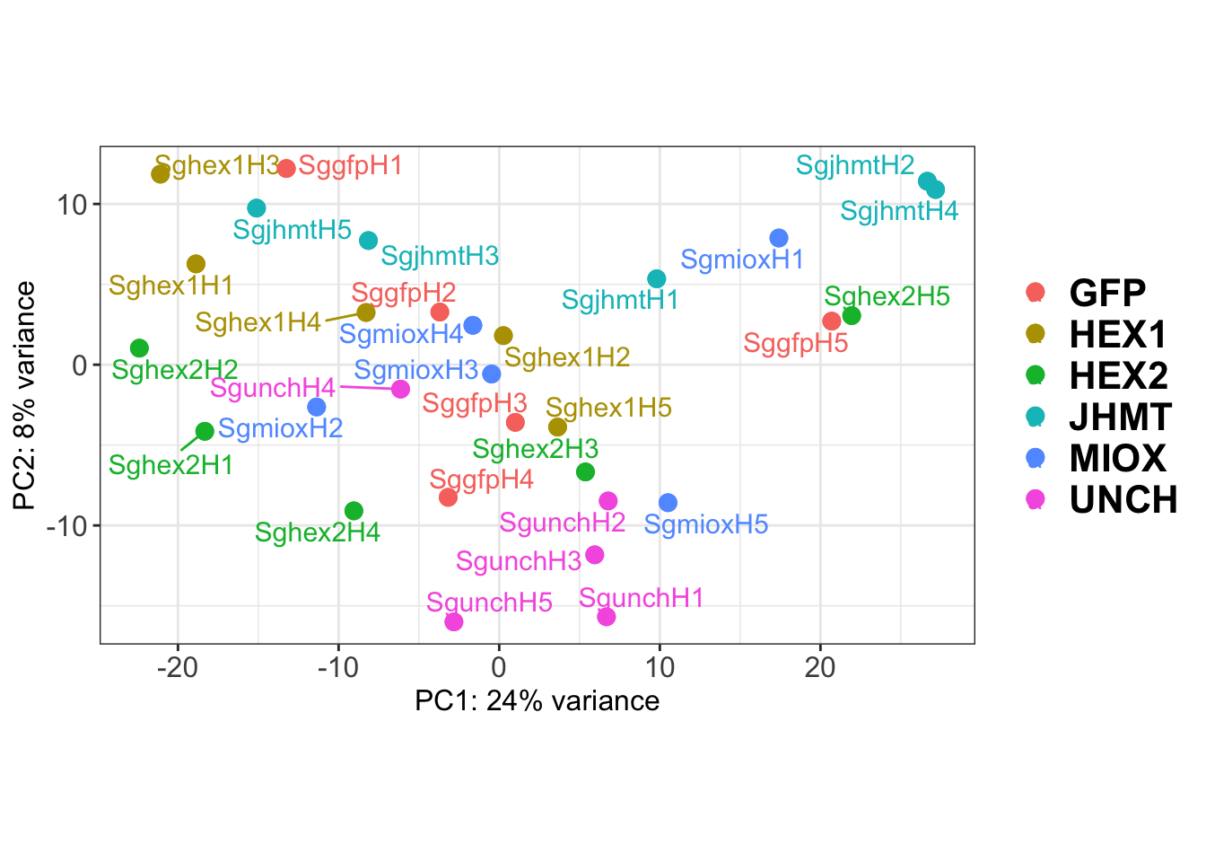
| Version | Author | Date |
|---|---|---|
| 3746422 | Maeva TECHER | 2025-02-12 |
ggsave(paste0(saveDir,"/PCA_labelled_plots.png"), width =10 , height = 10,
       dpi = 600, device = "png", plot = p1)

p2 <- plotPCA(vsd, intgroup=c("Gene")) +
  geom_point(size=3) +
  theme_bw() +
  theme(legend.title = element_blank()) +
  theme(legend.text = element_text(face="bold", size=16)) +
  theme(axis.text = element_text(size=12)) +
  theme(axis.title = element_text(size=12)) +
  geom_convexhull(aes(fill = Gene), alpha = 0.5) +
  ggtitle("PCA on S. gregaria Head tissues", subtitle = "vst transformation")
p2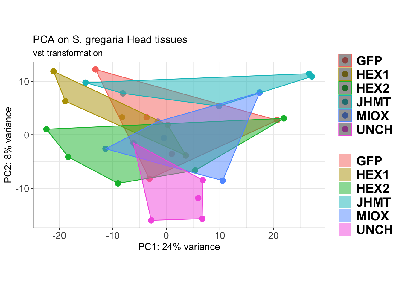
| Version | Author | Date |
|---|---|---|
| 3746422 | Maeva TECHER | 2025-02-12 |
ggsave(paste0(saveDir,"/PCA_plot.png"), width =10 , height = 10,
       dpi = 600, device = "png", plot = p2)
The PCA plot shows clear distinction between tissue types, while gene silencing has a large variation within each tissue, and presents no distinct clear groupings for a single gene.
Surrogate Variable Analysis
### SVA analysis to control for technical variation
dat <- counts(dds, normalized = TRUE)
idx <- rowMeans(dat) > 1
dat <- dat[idx, ]
mod <- model.matrix(~ Gene, colData(dds))
mod0 <- model.matrix(~ 1, colData(dds))
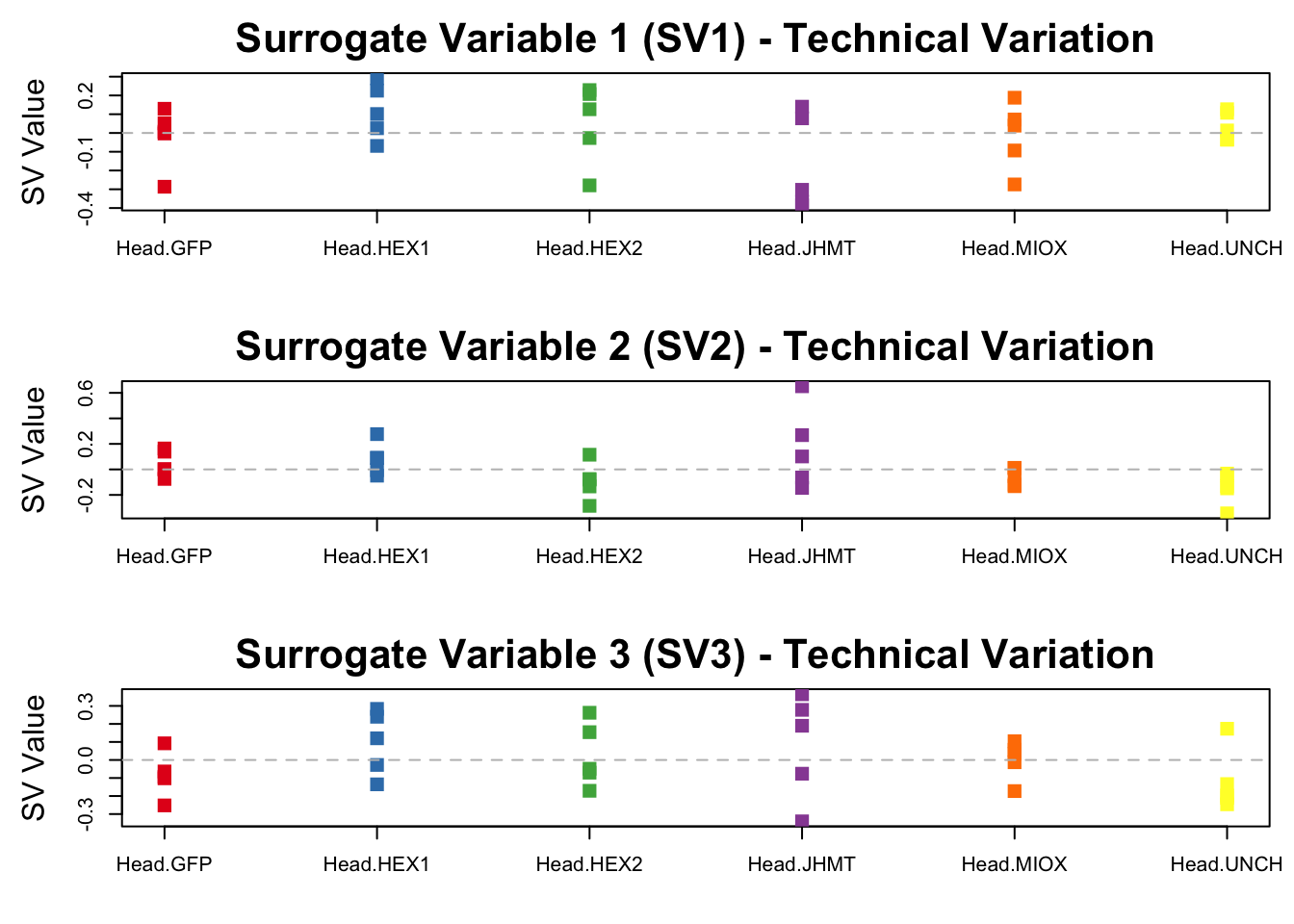
svseq <- svaseq(dat, mod, mod0)Number of significant surrogate variables is: 3
Iteration (out of 5 ):1 2 3 4 5 # Set up layout: 3 plots in a 3x1 grid
par(mfrow = c(3, 1), mar = c(4,5,3,1))
# Create color mapping for each unique combination of Tissue + Gene
tissue_gene_groups <- interaction(dds$Tissue, dds$Gene, drop = TRUE) # Create grouping
unique_groups <- unique(tissue_gene_groups) # Get unique combinations
group_colors <- setNames(colorRampPalette(brewer.pal(min(length(unique_groups), 8), "Set1"))(length(unique_groups)), unique_groups)
# Loop through first 3 surrogate variables
for (i in 1:3) {
# Extract SV values
sv_values <- svseq$sv[, i]
# Assign colors per group
assigned_colors <- group_colors[as.factor(tissue_gene_groups)]
stripchart(sv_values ~ tissue_gene_groups,
vertical = TRUE,
pch = 15, # Use solid circles
cex = 1.5, # Increase point size
col = group_colors, # Correctly map colors per group
main = paste0("Surrogate Variable ", i, " (SV", i, ") - Technical Variation"),
ylab = "SV Value",
cex.axis = 1, cex.lab = 1.5, cex.main = 2)
abline(h = 0, lty = 2, col = "gray") # Dashed reference line
}
| Version | Author | Date |
|---|---|---|
| 3746422 | Maeva TECHER | 2025-02-12 |
# Add a legend with correctly mapped colors
#legend("topright", legend = unique_groups, col = group_colors, pch = 16, cex = 1.2, bty = "n", title = "Tissue + Gene")

# Save the plot **AFTER** displaying it for knitr
dev.copy(png, filename = paste0(saveDir, "/sva_analysis.png"), width = 15000, height = 5000, res = 600)
quartz_off_screen
3 dev.off()quartz_off_screen
2 bigpar() # Optimize plotting parameters
# Set up layout: 3 rows, 1 column
par(mfrow = c(2, 2), mar = c(5, 5, 3, 2)) # Adjust margins for readability
# Generate color mapping for each unique Gene
gene_labels <- as.character(dds$Gene)
unique_genes <- unique(gene_labels)
gene_colors <- setNames(colorRampPalette(brewer.pal(min(length(unique_genes), 8), "Set1"))(length(unique_genes)), unique_genes)
# === Plot 1: SV1 vs SV2 ===
plot(svseq$sv[,1], svseq$sv[,2],
col = gene_colors[gene_labels],
pch = 16, cex = 1.5,
xlab = "SV1", ylab = "SV2",
main = "SVA Analysis: SV1 vs SV2")
# === Plot 2: SV1 vs SV3 ===
plot(svseq$sv[,1], svseq$sv[,3],
col = gene_colors[gene_labels],
pch = 16, cex = 1.5,
xlab = "SV1", ylab = "SV3",
main = "SVA Analysis: SV1 vs SV3")
# === Plot 3: SV2 vs SV3 ===
plot(svseq$sv[,2], svseq$sv[,3],
col = gene_colors[gene_labels],
pch = 16, cex = 1.5,
xlab = "SV2", ylab = "SV3",
main = "SVA Analysis: SV2 vs SV3")
# === Fourth Plot (Empty) with Legend ===
plot.new()
legend("topright", legend = unique_genes, pch = 16, col = gene_colors, cex = 1, title = "Gene", ncol = 3)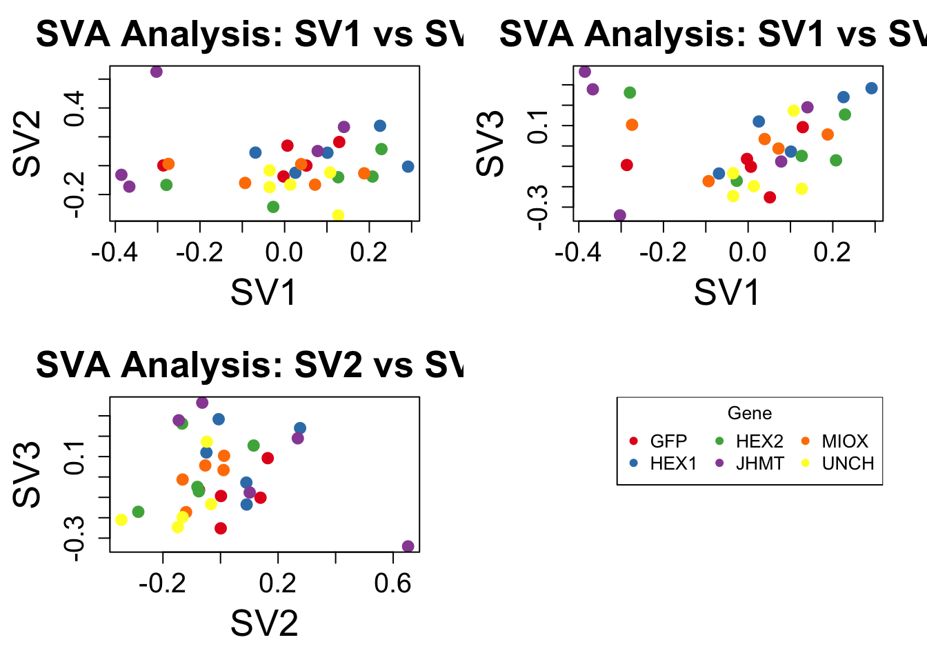
| Version | Author | Date |
|---|---|---|
| 3746422 | Maeva TECHER | 2025-02-12 |
dev.copy(png, filename = paste0(saveDir, "/sva_analysis_interact.png"), width = 15000, height = 5000, res = 600)quartz_off_screen
3 dev.off()quartz_off_screen
2 We rerun the DESeq2 model but this time including the
surrogate variable as a covariate, as we know that the modeled variation
is more likely explained by tissue and gene variation rather than batch
effects.
ddssva <- dds
ddssva$SV1 <- svseq$sv[,1]
ddssva$SV2 <- svseq$sv[,2]
ddssva$SV3 <- svseq$sv[,3]
design(ddssva) <- ~ SV1 + SV2 + SV3 + Gene
ddssva$Gene <- relevel(ddssva$Gene, ref = "GFP")

smallestGroupSize <- 5
keep <- rowSums(counts(ddssva) >= 10) >= smallestGroupSize
ddssva <- ddssva[keep,]

ddssva <- DESeq(ddssva)

ddssva <- ddssva[which(mcols(ddssva)$betaConv),] # remove non converging rows

### Extract results
resultsNames(ddssva)
[1] "Intercept" "SV1" "SV2" "SV3"
[5] "Gene_HEX1_vs_GFP" "Gene_HEX2_vs_GFP" "Gene_JHMT_vs_GFP" "Gene_MIOX_vs_GFP"
[9] "Gene_UNCH_vs_GFP"hex1 <- results(ddssva, name = "Gene_HEX1_vs_GFP", alpha = 0.05)
hex2 <- results(ddssva, name = "Gene_HEX2_vs_GFP", alpha = 0.05)
jhmt <- results(ddssva, name = "Gene_JHMT_vs_GFP", alpha = 0.05)
miox <- results(ddssva, name = "Gene_MIOX_vs_GFP", alpha = 0.05)
unch <- results(ddssva, name = "Gene_UNCH_vs_GFP", alpha = 0.05)Volcano plots and Heatmaps
First we create function to generate the plots we are interested to obtain and then run the whole pipeline for each gene.
create_output_dirs <- function(label) {
  dir.create(file.path(saveDir, label), showWarnings = FALSE)
  return()
}

# Retrieve various accession IDs
get_sig_genes <- function(res) {
  sig_genes <- res[which(res$padj < 0.05 & abs(res$log2FoldChange)>=1.0), ]
  sig_genes <- sig_genes[order(sig_genes, decreasing = T), ]
  return(sig_genes)
}

create_volcano <- function(res, label) {
  mypalette <- brewer.pal(9, "Set1")
  volcano <-EnhancedVolcano(res,
                            lab=rownames(res),
                            x='log2FoldChange',
                            y='padj',
                            title=paste("Volcano Plot:", label),
                            col=c(mypalette[9], mypalette[3], mypalette[2],
                                  mypalette[1]),
                            labSize = 4,
                            pCutoff = 0.05,
                            FCcutoff = 1,
                            pointSize = 3,
                            drawConnectors = T,
                            widthConnectors = 0.5,
                            colConnectors = "black",
                            max.overlaps = 25,
                            gridlines.major = F,
                            gridlines.minor = F)
  ggsave(paste0(saveDir, "/", label,"/volcano_plot_",label,".tiff"), device = "tiff",
         plot = volcano, width = 10, height = 10)
  return()
}

create_heatmap <- function(res, label, contrast_) {
  mat <- counts(dds, normalized=T)
  mat.z <- t(apply(mat, 1, scale))
  colnames(mat.z) <- colnames(mat)
  mat.z <- mat.z[rownames(res), contrast_, drop=F]
  rownames(mat.z) <- rownames(res)
  tiff(paste0(saveDir, "/", label,"/heatmap_plot_",label,".tiff"),
       units="in", res= 300, width =5, height=10 )
  draw(Heatmap(mat.z,
               cluster_rows = T,
               cluster_columns = F,
               column_labels = contrast_,
               name = "Z-Transformed Counts",
               row_labels = rownames(mat.z),
               row_names_gp = gpar(fontsize=8)))
  dev.off()
  return()
}


# Define contrast_sets
hex1_samples <- c("SggfpH1","SggfpH2","SggfpH3","SggfpH4","SggfpH5",
                  "Sghex1H1","Sghex1H2","Sghex1H3","Sghex1H4","Sghex1H5")
hex2_samples <- c("SggfpH1","SggfpH2","SggfpH3","SggfpH4","SggfpH5",
                  "Sghex2H1","Sghex2H2","Sghex2H3","Sghex2H4","Sghex2H5")
jhmt_samples <- c("SggfpH1","SggfpH2","SggfpH3","SggfpH4","SggfpH5",
                  "SgjhmtH1","SgjhmtH2","SgjhmtH3","SgjhmtH4","SgjhmtH5")
miox_samples <- c("SggfpH1","SggfpH2","SggfpH3","SggfpH4","SggfpH5",
                  "SgmioxH1","SgmioxH2","SgmioxH3","SgmioxH4","SgmioxH5")
unch_samples <- c("SggfpH1","SggfpH2","SggfpH3","SggfpH4","SggfpH5",
                  "SgunchH1","SgunchH2","SgunchH3","SgunchH4","SgunchH5")


visualize_data <- function(res, label, contrast_) {
  sig_genes <- get_sig_genes(res)
  create_output_dirs(label)
  write.csv(as.data.frame(sig_genes), paste0(saveDir, "/",label, "/DGE_results_", label,
                                             ".csv"))
  create_volcano(res, label)
  create_heatmap(sig_genes, label, contrast_)
  return()
}

# Run full analysis
visualize_data(hex1,
             "Hex1_vs_GFP",
hex1_samples)NULLvisualize_data(hex2,
"Hex2_vs_GFP",
hex2_samples)NULLvisualize_data(jhmt,
"JHMT_vs_GFP",
jhmt_samples)NULLvisualize_data(miox,
"MIOX_vs_GFP",
miox_samples)NULLvisualize_data(unch,
"UNCH_vs_GFP",
unch_samples)NULLGO and KEGG enrichment
get_ids <- function(res) {
  rownames(res) <- as.character(rownames(res))
  res$ensembl_gene_id <- row.names(res)
  annotations <- getBM(attributes = c("ensembl_gene_id", "geneid"),
                       filters = "ensembl_gene_id",
                       values = rownames(res),
                       mart = dataset)
  return(annotations$geneid)
}

GOMFEnrichment <- function(res, label) {
  # Check if there are valid gene IDs
  if (!is.null(res)) {

    # Perform GO enrichment analysis
    ego <- enrichGO(
      gene = rownames(res),
      OrgDb = org.Sgregaria.eg.db,
      keyType = "GID",
      ont = "MF",  # Cellular Component
      pAdjustMethod = "BH",  # Benjamini-Hochberg adjustment
      pvalueCutoff = 0.1
    )

    # Check if the result has any significant enrichment terms
    if (nrow(as.data.frame(ego)) > 0) {
      # Create the barplot
      go_barplot <- barplot(ego, showCategory = 20) +  # Show top 20 categories
        ggtitle(paste("GO MF Enrichment:", label))

      # Print the plot
      ggsave(paste0(save_dir, "/", label,"/gp_MF_barplot_",label,".tiff"), device = "tiff",
             plot=go_barplot, width=10, height = 10)

      change_vec <- res$log2FoldChange
      names(change_vec) <- rownames(res)
      RYD  = brewer.pal(n = 8, name = "RdBu")
      go_network <- cnetplot(ego, foldChange=change_vec) +
        scale_color_gradientn(colours = RYD, limits=c(-2,2))
      ggsave(paste0(save_dir, "/", label,"/gp_MF_cnetplot_",label,".tiff"), device = "tiff",
             plot=go_network, width=30, height = 30, bg = "white")

      write.csv(as.data.frame(ego), paste0(save_dir, "/", label,
                                           "/GO_MF_Enrichment_Results_", label,".csv"))
    } else {
      message("No significant MF GO terms found.")
    }

  } else {
    message("No valid gene IDs found.")
  }
  return()
}

GOCCEnrichment <- function(res, label) {
  # Check if there are valid gene IDs
  if (!is.null(res)) {

    # Perform GO enrichment analysis
    ego <- enrichGO(
      gene = rownames(res),
      OrgDb = org.Sgregaria.eg.db,
      keyType = "GID",
      ont = "CC",  # Cellular Component
      pAdjustMethod = "BH",  # Benjamini-Hochberg adjustment
      pvalueCutoff = 0.1
    )

    # Check if the result has any significant enrichment terms
    if (nrow(as.data.frame(ego)) > 0) {
      # Create the barplot
      go_barplot <- barplot(ego, showCategory = 20) +  # Show top 20 categories
        ggtitle(paste("GO CC Enrichment:", label))

      # Print the plot
      ggsave(paste0(save_dir, "/", label,"/gp_CC_barplot_",label,".tiff"), device = "tiff",
             plot=go_barplot, width=10, height = 10)

      change_vec <- res$log2FoldChange
      names(change_vec) <- rownames(res)
      RYD  = brewer.pal(n = 8, name = "RdBu")
      go_network <- cnetplot(ego, foldChange=change_vec) +
        scale_color_gradientn(colours = RYD, limits=c(-2,2))
      ggsave(paste0(save_dir, "/", label,"/gp_CC_cnetplot_",label,".tiff"), device = "tiff",
             plot=go_network, width=30, height = 30, bg = "white")

      write.csv(as.data.frame(ego), paste0(save_dir, "/", label,
                                           "/GO_CC_Enrichment_Results_", label,".csv"))
    } else {
      message("No significant CC GO terms found.")
    }

  } else {
    message("No valid gene IDs found.")
  }
  return()
}

GOBPEnrichment <- function(res, label) {
  # Check if there are valid gene IDs
  if (!is.null(res)) {

    # Perform GO enrichment analysis
    ego <- enrichGO(
      gene = rownames(res),
      OrgDb = org.Sgregaria.eg.db,
      keyType = "GID",
      ont = "BP",  # Cellular Component
      pAdjustMethod = "BH",  # Benjamini-Hochberg adjustment
      pvalueCutoff = 0.1
    )

    # Check if the result has any significant enrichment terms
    if (nrow(as.data.frame(ego)) > 0) {
      # Create the barplot
      go_barplot <- barplot(ego, showCategory = 20) +  # Show top 20 categories
        ggtitle(paste("GO BP Enrichment:", label))

      # Print the plot
      ggsave(paste0(save_dir, "/", label,"/gp_BP_barplot_",label,".tiff"), device = "tiff",
             plot=go_barplot, width=10, height = 10)

      change_vec <- res$log2FoldChange
      names(change_vec) <- rownames(res)
      RYD  = brewer.pal(n = 8, name = "RdBu")
      go_network <- cnetplot(ego, foldChange=change_vec) +
        scale_color_gradientn(colours = RYD, limits=c(-2,2))
      ggsave(paste0(save_dir, "/", label,"/gp_BP_cnetplot_",label,".tiff"), device = "tiff",
             plot=go_network, width=30, height = 30, bg="white")

      write.csv(as.data.frame(ego), paste0(save_dir, "/", label,
                                           "/GO_BP_Enrichment_Results_", label,".csv"))
    } else {
      message("No significant BP GO terms found.")
    }

  } else {
    message("No valid gene IDs found.")
  }
  return()
}

KEGGEnrichment <- function(res, label) {
  # Check if there are valid gene IDs
  if (!is.null(res)) {

    kk <- enrichKEGG(gene = rownames(res),
                     organism = "sgre",
                     pvalueCutoff = 0.1)

    # Check if the result has any significant enrichment terms
    if (nrow(as.data.frame(kk)) > 0) {

      kk_barplot <- barplot(kk) + ggtitle(paste("KEGG Enrichment:", label))
      ggsave(paste0(save_dir, "/", label,"/kk_barplot_",label,".tiff"), device = "tiff",
             plot=kk_barplot, width=10, height = 10)

      change_vec <- res$log2FoldChange
      names(change_vec) <- rownames(res)
      RYD  = brewer.pal(n = 8, name = "RdBu")
      kk_network <- cnetplot(kk, foldChange=change_vec) +
        scale_color_gradientn(colours = RYD, limits=c(-2,2))
      ggsave(paste0(save_dir, "/", label,"/kk_cnetplot_",label,".tiff"), device = "tiff",
             plot=kk_network, width=30, height = 30, bg = "white")

      write.csv(as.data.frame(kk), paste0(save_dir,  "/",label,
                                          "/KEGG_Enrichment_Results_",
                                          label,".csv"))
    } else {
      message("No significant KEGG terms found.")
    }

  } else {
    message("No valid gene IDs found.")
  }
  return()
}

enrich_data <- function(res, label, contrast_) {
  sig_genes <- get_sig_genes(res)
  create_output_dirs(label)
  GOMFEnrichment(sig_genes, label)
  GOBPEnrichment(sig_genes, label)
  GOCCEnrichment(sig_genes, label)
  KEGGEnrichment(sig_genes, label)
  return()
}

#enrich_data(hex1, "Hex1_vs_GFP", hex1_samples)
#enrich_data(hex2,"Hex2_vs_GFP", hex2_samples)
#enrich_data(jhmt,"JHMT_vs_GFP",jhmt_samples)
#enrich_data(miox,"MIOX_vs_GFP",miox_samples)
#enrich_data(unch,"UNCH_vs_GFP",unch_samples)
Thorax tissue
saveDir <- paste0(workDir,"/DEG_results/RNAi/Thorax")
dir.create(saveDir)

### Prepare Sample CSV file #####
samples <- read.delim(file.path(workDir, "list/RNAi/Thorax_RNAisample_list.csv"), sep = ",", row.names = 1, header = TRUE)
files <- file.path(workDir, "readcounts/RNAi/", samples$Tissue, samples$Filename)
names(files) <- row.names(samples)
all(file.exists(files))
[1] TRUE### Create count sample matrix
cts <- map_dfc(files, function(sample) {
data_count <- read.delim(sample, sep = "\t", header = FALSE)
col_name <- gsub("_counts.txt", "", basename(sample))
setNames(data.frame(data_count[, 2]), col_name)
})
row_get <- read.delim(files[1], sep = "\t", row.names = 1, header = F) # Get proper row names
rownames(cts) <- rownames(row_get)
rm(row_get) # remove unused object from memoryWhile for bulk RNAseq on head and thorax for all species, the DEGs model was made between isolated and crowded individuals (with isolated as the reference state), here, the DEG analysis will be carried between GFP knock-down nymphs (as reference state) vs Hexamerins / Juvenile Hormones / Uncharacterized proteins
### Build DESeq2 Object
dds <- DESeqDataSetFromMatrix(countData = cts,
                              colData = samples,
                              design = ~ Gene)
dds$Gene <- relevel(dds$Gene, ref = "GFP")

smallestGroupSize <- 5
keep <- rowSums(counts(dds) >= 10) >= smallestGroupSize
dds <- dds[keep,]

dds <- DESeq(dds)
Following the generation of the DEseq2 object, we
annotate the genes with the GeneID using biomaRt.
### Fetch Annotation Gene IDs using biomaRt
ensembl <- useMart("metazoa_mart", host = "https://metazoa.ensembl.org")
metazoa_list <- listDatasets(ensembl)
dataset <- useMart("metazoa_mart", dataset = "sggca023897955v2rs_eg_gene",
                   host = "https://metazoa.ensembl.org")
#listAttributes(dataset)

test_raw_counts <- as.data.frame(counts(dds))
rownames(test_raw_counts) <- as.character(rownames(test_raw_counts))
test_raw_counts$ensembl_gene_id <- row.names(test_raw_counts)
annotations <- getBM(attributes = c("ensembl_gene_id", "geneid"),
                     filters = "ensembl_gene_id",
                     values = rownames(test_raw_counts),
                     mart = dataset)

# Merge dataframes to retain geneid information from biomaRt
test_raw_counts_annotated <- merge(test_raw_counts, annotations,
                                   by = "ensembl_gene_id",
                                   all.x = T)

write.csv(test_raw_counts_annotated, file=paste0(saveDir,"/Thorax_raw_counts.csv"))
#####
Normalization and PCA
# Plot PCA and investigate quality metrics
vsd <- vst(dds, blind=T)

p1 <- plotPCA(vsd, intgroup=c("Gene")) +
  geom_text_repel(aes(label = rownames(samples)), size = 4, max.overlaps = 20) +
  geom_point(size=3) +
  theme_bw() +
  theme(legend.title = element_blank()) +
  theme(legend.text = element_text(face="bold", size=16)) +
  theme(axis.text = element_text(size=12)) +
  theme(axis.title = element_text(size=12))
p1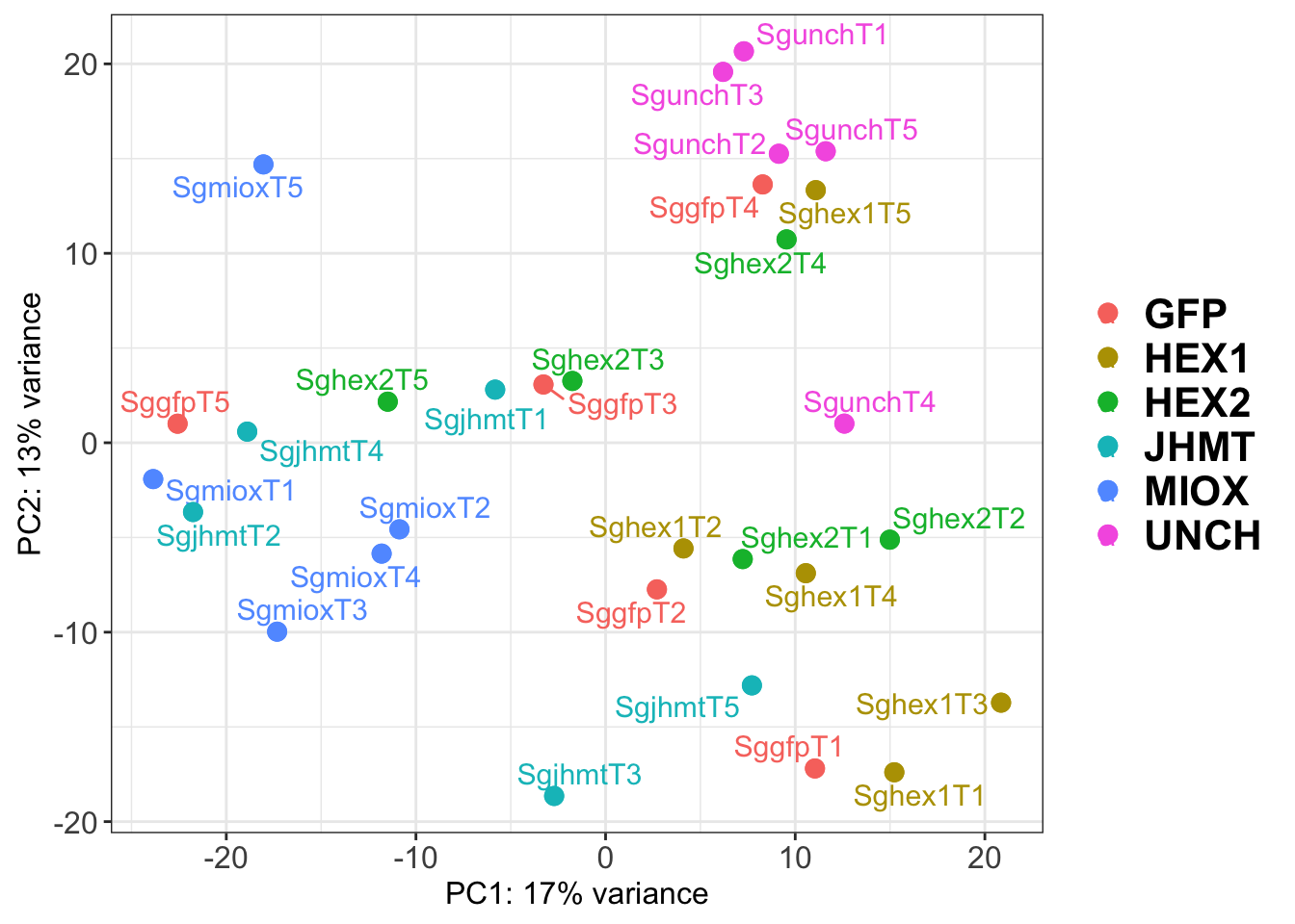
| Version | Author | Date |
|---|---|---|
| 3746422 | Maeva TECHER | 2025-02-12 |
ggsave(paste0(saveDir,"/PCA_labelled_plots.png"), width =10 , height = 10,
       dpi = 600, device = "png", plot = p1)

p2 <- plotPCA(vsd, intgroup=c("Gene")) +
  geom_point(size=3) +
  theme_bw() +
  theme(legend.title = element_blank()) +
  theme(legend.text = element_text(face="bold", size=16)) +
  theme(axis.text = element_text(size=12)) +
  theme(axis.title = element_text(size=12)) +
  geom_convexhull(aes(fill = Gene), alpha = 0.5) +
  ggtitle("PCA on S. gregaria Thorax tissues", subtitle = "vst transformation")
p2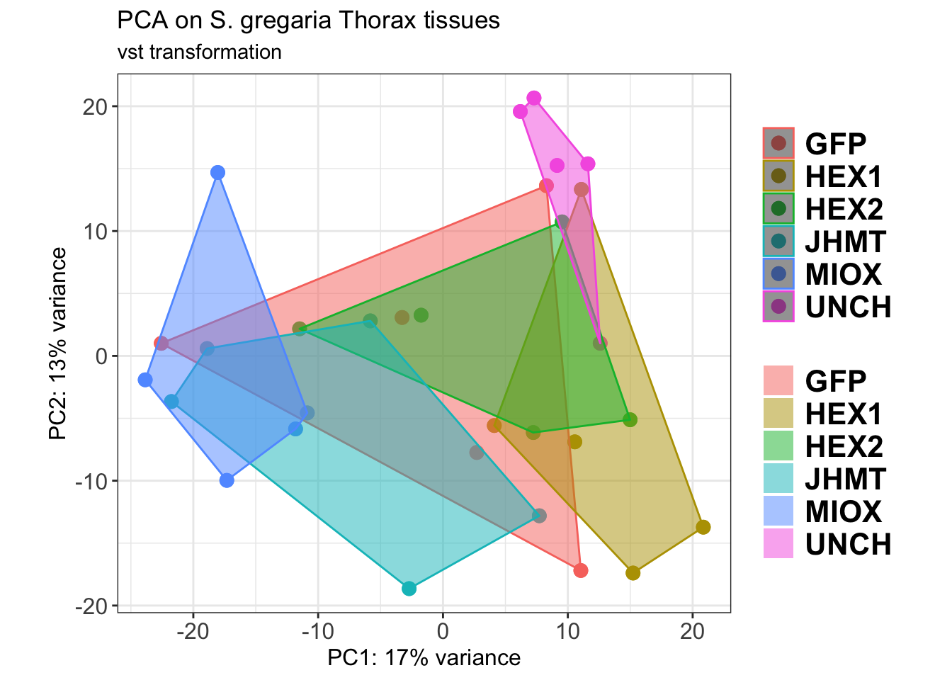
| Version | Author | Date |
|---|---|---|
| 3746422 | Maeva TECHER | 2025-02-12 |
ggsave(paste0(saveDir,"/PCA_plot.png"), width =10 , height = 10,
       dpi = 600, device = "png", plot = p2)
The PCA plot shows clear distinction between tissue types, while gene silencing has a large variation within each tissue, and presents no distinct clear groupings for a single gene.
Surrogate Variable Analysis
### SVA analysis to control for technical variation
dat <- counts(dds, normalized = TRUE)
idx <- rowMeans(dat) > 1
dat <- dat[idx, ]
mod <- model.matrix(~ Gene, colData(dds))
mod0 <- model.matrix(~ 1, colData(dds))
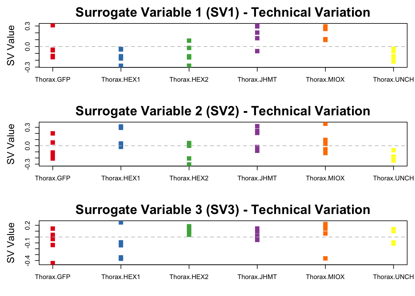
svseq <- svaseq(dat, mod, mod0)Number of significant surrogate variables is: 4
Iteration (out of 5 ):1 2 3 4 5 # Set up layout: 3 plots in a 3x1 grid
par(mfrow = c(3, 1), mar = c(4,5,3,1))
# Create color mapping for each unique combination of Tissue + Gene
tissue_gene_groups <- interaction(dds$Tissue, dds$Gene, drop = TRUE) # Create grouping
unique_groups <- unique(tissue_gene_groups) # Get unique combinations
group_colors <- setNames(colorRampPalette(brewer.pal(min(length(unique_groups), 8), "Set1"))(length(unique_groups)), unique_groups)
# Loop through first 3 surrogate variables
for (i in 1:3) {
# Extract SV values
sv_values <- svseq$sv[, i]
# Assign colors per group
assigned_colors <- group_colors[as.factor(tissue_gene_groups)]
stripchart(sv_values ~ tissue_gene_groups,
vertical = TRUE,
pch = 15, # Use solid circles
cex = 1.5, # Increase point size
col = group_colors, # Correctly map colors per group
main = paste0("Surrogate Variable ", i, " (SV", i, ") - Technical Variation"),
ylab = "SV Value",
cex.axis = 1, cex.lab = 1.5, cex.main = 2)
abline(h = 0, lty = 2, col = "gray") # Dashed reference line
}
| Version | Author | Date |
|---|---|---|
| 3746422 | Maeva TECHER | 2025-02-12 |
# Add a legend with correctly mapped colors
#legend("topright", legend = unique_groups, col = group_colors, pch = 16, cex = 1.2, bty = "n", title = "Tissue + Gene")

# Save the plot **AFTER** displaying it for knitr
dev.copy(png, filename = paste0(saveDir, "/sva_analysis.png"), width = 15000, height = 5000, res = 600)
quartz_off_screen
3 dev.off()quartz_off_screen
2 bigpar() # Optimize plotting parameters
# Set up layout: 3 rows, 1 column
par(mfrow = c(2, 2), mar = c(5, 5, 3, 2)) # Adjust margins for readability
# Generate color mapping for each unique Gene
gene_labels <- as.character(dds$Gene)
unique_genes <- unique(gene_labels)
gene_colors <- setNames(colorRampPalette(brewer.pal(min(length(unique_genes), 8), "Set1"))(length(unique_genes)), unique_genes)
# === Plot 1: SV1 vs SV2 ===
plot(svseq$sv[,1], svseq$sv[,2],
col = gene_colors[gene_labels],
pch = 16, cex = 1.5,
xlab = "SV1", ylab = "SV2",
main = "SVA Analysis: SV1 vs SV2")
# === Plot 2: SV1 vs SV3 ===
plot(svseq$sv[,1], svseq$sv[,3],
col = gene_colors[gene_labels],
pch = 16, cex = 1.5,
xlab = "SV1", ylab = "SV3",
main = "SVA Analysis: SV1 vs SV3")
# === Plot 3: SV2 vs SV3 ===
plot(svseq$sv[,2], svseq$sv[,3],
col = gene_colors[gene_labels],
pch = 16, cex = 1.5,
xlab = "SV2", ylab = "SV3",
main = "SVA Analysis: SV2 vs SV3")
# === Fourth Plot (Empty) with Legend ===
plot.new()
legend("topright", legend = unique_genes, pch = 16, col = gene_colors, cex = 1, title = "Gene", ncol = 3)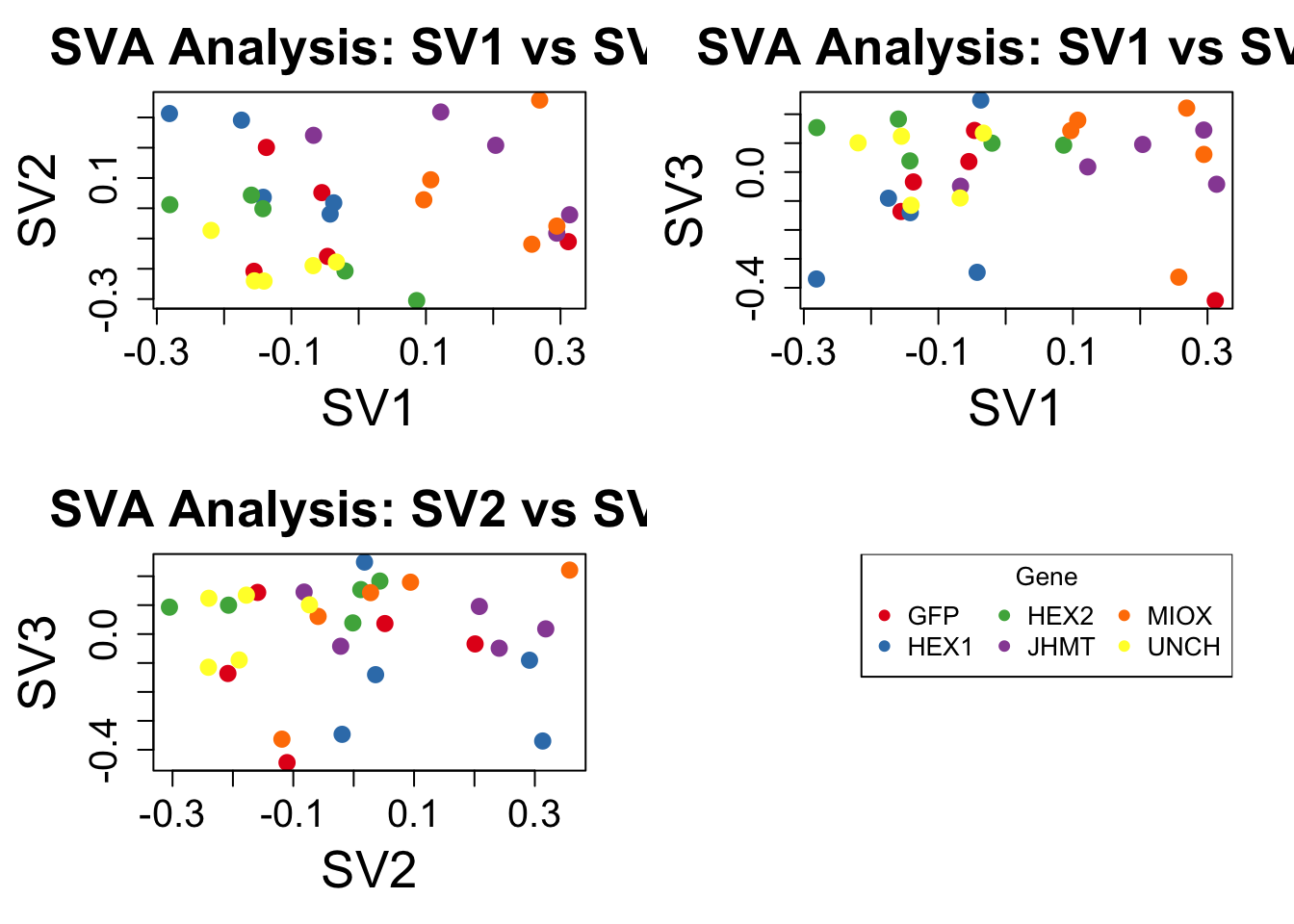
| Version | Author | Date |
|---|---|---|
| 3746422 | Maeva TECHER | 2025-02-12 |
dev.copy(png, filename = paste0(saveDir, "/sva_analysis_interact.png"), width = 15000, height = 5000, res = 600)quartz_off_screen
3 dev.off()quartz_off_screen
2 We rerun the DESeq2 model but this time including the
surrogate variable as a covariate, as we know that the modeled variation
is more likely explained by tissue and gene variation rather than batch
effects.
ddssva <- dds
ddssva$SV1 <- svseq$sv[,1]
ddssva$SV2 <- svseq$sv[,2]
ddssva$SV3 <- svseq$sv[,3]
design(ddssva) <- ~ SV1 + SV2 + SV3 + Gene
ddssva$Gene <- relevel(ddssva$Gene, ref = "GFP")

smallestGroupSize <- 5
keep <- rowSums(counts(ddssva) >= 10) >= smallestGroupSize
ddssva <- ddssva[keep,]

ddssva <- DESeq(ddssva)

ddssva <- ddssva[which(mcols(ddssva)$betaConv),] # remove non converging rows

### Extract results
resultsNames(ddssva)
[1] "Intercept" "SV1" "SV2" "SV3"
[5] "Gene_HEX1_vs_GFP" "Gene_HEX2_vs_GFP" "Gene_JHMT_vs_GFP" "Gene_MIOX_vs_GFP"
[9] "Gene_UNCH_vs_GFP"hex1 <- results(ddssva, name = "Gene_HEX1_vs_GFP", alpha = 0.05)
hex2 <- results(ddssva, name = "Gene_HEX2_vs_GFP", alpha = 0.05)
jhmt <- results(ddssva, name = "Gene_JHMT_vs_GFP", alpha = 0.05)
miox <- results(ddssva, name = "Gene_MIOX_vs_GFP", alpha = 0.05)
unch <- results(ddssva, name = "Gene_UNCH_vs_GFP", alpha = 0.05)Volcano plots and Heatmaps
First we create function to generate the plots we are interested to obtain and then run the whole pipeline for each gene.
create_output_dirs <- function(label) {
  dir.create(file.path(saveDir, label), showWarnings = FALSE)
  return()
}

# Retrieve various accession IDs
get_sig_genes <- function(res) {
  sig_genes <- res[which(res$padj < 0.05 & abs(res$log2FoldChange)>=1.0), ]
  sig_genes <- sig_genes[order(sig_genes, decreasing = T), ]
  return(sig_genes)
}

create_volcano <- function(res, label) {
  mypalette <- brewer.pal(9, "Set1")
  volcano <-EnhancedVolcano(res,
                            lab=rownames(res),
                            x='log2FoldChange',
                            y='padj',
                            title=paste("Volcano Plot:", label),
                            col=c(mypalette[9], mypalette[3], mypalette[2],
                                  mypalette[1]),
                            labSize = 4,
                            pCutoff = 0.05,
                            FCcutoff = 1,
                            pointSize = 3,
                            drawConnectors = T,
                            widthConnectors = 0.5,
                            colConnectors = "black",
                            max.overlaps = 25,
                            gridlines.major = F,
                            gridlines.minor = F)
  ggsave(paste0(saveDir, "/", label,"/volcano_plot_",label,".tiff"), device = "tiff",
         plot = volcano, width = 10, height = 10)
  return()
}

create_heatmap <- function(res, label, contrast_) {
  mat <- counts(dds, normalized=T)
  mat.z <- t(apply(mat, 1, scale))
  colnames(mat.z) <- colnames(mat)
  mat.z <- mat.z[rownames(res), contrast_, drop=F]
  rownames(mat.z) <- rownames(res)
  tiff(paste0(saveDir, "/", label,"/heatmap_plot_",label,".tiff"),
       units="in", res= 300, width =5, height=10 )
  draw(Heatmap(mat.z,
               cluster_rows = T,
               cluster_columns = F,
               column_labels = contrast_,
               name = "Z-Transformed Counts",
               row_labels = rownames(mat.z),
               row_names_gp = gpar(fontsize=8)))
  dev.off()
  return()
}


# Define contrast_sets
hex1_samples <- c("SggfpT1","SggfpT2","SggfpT3","SggfpT4","SggfpT5",
                  "Sghex1T1","Sghex1T2","Sghex1T3","Sghex1T4","Sghex1T5")
hex2_samples <- c("SggfpT1","SggfpT2","SggfpT3","SggfpT4","SggfpT5",
                  "Sghex2T1","Sghex2T2","Sghex2T3","Sghex2T4","Sghex2T5")
jhmt_samples <- c("SggfpT1","SggfpT2","SggfpT3","SggfpT4","SggfpT5",
                  "SgjhmtT1","SgjhmtT2","SgjhmtT3","SgjhmtT4","SgjhmtT5")
miox_samples <- c("SggfpT1","SggfpT2","SggfpT3","SggfpT4","SggfpT5",
                  "SgmioxT1","SgmioxT2","SgmioxT3","SgmioxT4","SgmioxT5")
unch_samples <- c("SggfpT1","SggfpT2","SggfpT3","SggfpT4","SggfpT5",
                  "SgunchT1","SgunchT2","SgunchT3","SgunchT4","SgunchT5")


visualize_data <- function(res, label, contrast_) {
  sig_genes <- get_sig_genes(res)
  create_output_dirs(label)
  write.csv(as.data.frame(sig_genes), paste0(saveDir, "/",label, "/DGE_results_", label,".csv"))
  create_volcano(res, label)
  create_heatmap(sig_genes, label, contrast_)
  return()
}

# Run full analysis
visualize_data(hex1,
             "Hex1_vs_GFP",
hex1_samples)NULLvisualize_data(hex2,
"Hex2_vs_GFP",
hex2_samples)NULLvisualize_data(jhmt,
"JHMT_vs_GFP",
jhmt_samples)NULLvisualize_data(miox,
"MIOX_vs_GFP",
miox_samples)NULLvisualize_data(unch,
"UNCH_vs_GFP",
unch_samples)NULLGO and KEGG enrichment
get_ids <- function(res) {
  rownames(res) <- as.character(rownames(res))
  res$ensembl_gene_id <- row.names(res)
  annotations <- getBM(attributes = c("ensembl_gene_id", "geneid"),
                       filters = "ensembl_gene_id",
                       values = rownames(res),
                       mart = dataset)
  return(annotations$geneid)
}

GOMFEnrichment <- function(res, label) {
  # Check if there are valid gene IDs
  if (!is.null(res)) {

    # Perform GO enrichment analysis
    ego <- enrichGO(
      gene = rownames(res),
      OrgDb = org.Sgregaria.eg.db,
      keyType = "GID",
      ont = "MF",  # Cellular Component
      pAdjustMethod = "BH",  # Benjamini-Hochberg adjustment
      pvalueCutoff = 0.1
    )

    # Check if the result has any significant enrichment terms
    if (nrow(as.data.frame(ego)) > 0) {
      # Create the barplot
      go_barplot <- barplot(ego, showCategory = 20) +  # Show top 20 categories
        ggtitle(paste("GO MF Enrichment:", label))

      # Print the plot
      ggsave(paste0(save_dir, "/", label,"/gp_MF_barplot_",label,".tiff"), device = "tiff",
             plot=go_barplot, width=10, height = 10)

      change_vec <- res$log2FoldChange
      names(change_vec) <- rownames(res)
      RYD  = brewer.pal(n = 8, name = "RdBu")
      go_network <- cnetplot(ego, foldChange=change_vec) +
        scale_color_gradientn(colours = RYD, limits=c(-2,2))
      ggsave(paste0(save_dir, "/", label,"/gp_MF_cnetplot_",label,".tiff"), device = "tiff",
             plot=go_network, width=30, height = 30, bg = "white")

      write.csv(as.data.frame(ego), paste0(save_dir, "/", label,
                                           "/GO_MF_Enrichment_Results_", label,".csv"))
    } else {
      message("No significant MF GO terms found.")
    }

  } else {
    message("No valid gene IDs found.")
  }
  return()
}

GOCCEnrichment <- function(res, label) {
  # Check if there are valid gene IDs
  if (!is.null(res)) {

    # Perform GO enrichment analysis
    ego <- enrichGO(
      gene = rownames(res),
      OrgDb = org.Sgregaria.eg.db,
      keyType = "GID",
      ont = "CC",  # Cellular Component
      pAdjustMethod = "BH",  # Benjamini-Hochberg adjustment
      pvalueCutoff = 0.1
    )

    # Check if the result has any significant enrichment terms
    if (nrow(as.data.frame(ego)) > 0) {
      # Create the barplot
      go_barplot <- barplot(ego, showCategory = 20) +  # Show top 20 categories
        ggtitle(paste("GO CC Enrichment:", label))

      # Print the plot
      ggsave(paste0(save_dir, "/", label,"/gp_CC_barplot_",label,".tiff"), device = "tiff",
             plot=go_barplot, width=10, height = 10)

      change_vec <- res$log2FoldChange
      names(change_vec) <- rownames(res)
      RYD  = brewer.pal(n = 8, name = "RdBu")
      go_network <- cnetplot(ego, foldChange=change_vec) +
        scale_color_gradientn(colours = RYD, limits=c(-2,2))
      ggsave(paste0(save_dir, "/", label,"/gp_CC_cnetplot_",label,".tiff"), device = "tiff",
             plot=go_network, width=30, height = 30, bg = "white")

      write.csv(as.data.frame(ego), paste0(save_dir, "/", label,
                                           "/GO_CC_Enrichment_Results_", label,".csv"))
    } else {
      message("No significant CC GO terms found.")
    }

  } else {
    message("No valid gene IDs found.")
  }
  return()
}

GOBPEnrichment <- function(res, label) {
  # Check if there are valid gene IDs
  if (!is.null(res)) {

    # Perform GO enrichment analysis
    ego <- enrichGO(
      gene = rownames(res),
      OrgDb = org.Sgregaria.eg.db,
      keyType = "GID",
      ont = "BP",  # Cellular Component
      pAdjustMethod = "BH",  # Benjamini-Hochberg adjustment
      pvalueCutoff = 0.1
    )

    # Check if the result has any significant enrichment terms
    if (nrow(as.data.frame(ego)) > 0) {
      # Create the barplot
      go_barplot <- barplot(ego, showCategory = 20) +  # Show top 20 categories
        ggtitle(paste("GO BP Enrichment:", label))

      # Print the plot
      ggsave(paste0(save_dir, "/", label,"/gp_BP_barplot_",label,".tiff"), device = "tiff",
             plot=go_barplot, width=10, height = 10)

      change_vec <- res$log2FoldChange
      names(change_vec) <- rownames(res)
      RYD  = brewer.pal(n = 8, name = "RdBu")
      go_network <- cnetplot(ego, foldChange=change_vec) +
        scale_color_gradientn(colours = RYD, limits=c(-2,2))
      ggsave(paste0(save_dir, "/", label,"/gp_BP_cnetplot_",label,".tiff"), device = "tiff",
             plot=go_network, width=30, height = 30, bg="white")

      write.csv(as.data.frame(ego), paste0(save_dir, "/", label,
                                           "/GO_BP_Enrichment_Results_", label,".csv"))
    } else {
      message("No significant BP GO terms found.")
    }

  } else {
    message("No valid gene IDs found.")
  }
  return()
}

KEGGEnrichment <- function(res, label) {
  # Check if there are valid gene IDs
  if (!is.null(res)) {

    kk <- enrichKEGG(gene = rownames(res),
                     organism = "sgre",
                     pvalueCutoff = 0.1)

    # Check if the result has any significant enrichment terms
    if (nrow(as.data.frame(kk)) > 0) {

      kk_barplot <- barplot(kk) + ggtitle(paste("KEGG Enrichment:", label))
      ggsave(paste0(save_dir, "/", label,"/kk_barplot_",label,".tiff"), device = "tiff",
             plot=kk_barplot, width=10, height = 10)

      change_vec <- res$log2FoldChange
      names(change_vec) <- rownames(res)
      RYD  = brewer.pal(n = 8, name = "RdBu")
      kk_network <- cnetplot(kk, foldChange=change_vec) +
        scale_color_gradientn(colours = RYD, limits=c(-2,2))
      ggsave(paste0(save_dir, "/", label,"/kk_cnetplot_",label,".tiff"), device = "tiff",
             plot=kk_network, width=30, height = 30, bg = "white")

      write.csv(as.data.frame(kk), paste0(save_dir,  "/",label,
                                          "/KEGG_Enrichment_Results_",
                                          label,".csv"))
    } else {
      message("No significant KEGG terms found.")
    }

  } else {
    message("No valid gene IDs found.")
  }
  return()
}

enrich_data <- function(res, label, contrast_) {
  sig_genes <- get_sig_genes(res)
  create_output_dirs(label)
  GOMFEnrichment(sig_genes, label)
  GOBPEnrichment(sig_genes, label)
  GOCCEnrichment(sig_genes, label)
  KEGGEnrichment(sig_genes, label)
  return()
}

#enrich_data(hex1, "Hex1_vs_GFP", hex1_samples)
#enrich_data(hex2,"Hex2_vs_GFP", hex2_samples)
#enrich_data(jhmt,"JHMT_vs_GFP",jhmt_samples)
#enrich_data(miox,"MIOX_vs_GFP",miox_samples)
#enrich_data(unch,"UNCH_vs_GFP",unch_samples)
sessionInfo()R version 4.4.1 (2024-06-14)
Platform: aarch64-apple-darwin20
Running under: macOS 15.3
Matrix products: default
BLAS: /Library/Frameworks/R.framework/Versions/4.4-arm64/Resources/lib/libRblas.0.dylib
LAPACK: /Library/Frameworks/R.framework/Versions/4.4-arm64/Resources/lib/libRlapack.dylib; LAPACK version 3.12.0
locale:
[1] en_US.UTF-8/en_US.UTF-8/en_US.UTF-8/C/en_US.UTF-8/en_US.UTF-8
time zone: Asia/Tokyo
tzcode source: internal
attached base packages:
[1] grid stats4 stats graphics grDevices utils datasets
[8] methods base
other attached packages:
[1] rafalib_1.0.0 biomaRt_2.60.1
[3] httr2_1.1.0 purrr_1.0.4
[5] dplyr_1.1.4 ashr_2.2-63
[7] cowplot_1.1.3 sva_3.52.0
[9] BiocParallel_1.38.0 genefilter_1.86.0
[11] mgcv_1.9-1 nlme_3.1-167
[13] clusterProfiler_4.12.6 EnhancedVolcano_1.22.0
[15] circlize_0.4.16 RColorBrewer_1.1-3
[17] ComplexHeatmap_2.20.0 ensembldb_2.28.1
[19] AnnotationFilter_1.28.0 GenomicFeatures_1.56.0
[21] AnnotationDbi_1.66.0 AnnotationHub_3.12.0
[23] BiocFileCache_2.12.0 dbplyr_2.5.0
[25] ggConvexHull_0.1.0 ggrepel_0.9.6
[27] ggplot2_3.5.1 DESeq2_1.44.0
[29] SummarizedExperiment_1.34.0 Biobase_2.64.0
[31] MatrixGenerics_1.16.0 matrixStats_1.5.0
[33] GenomicRanges_1.56.2 GenomeInfoDb_1.40.1
[35] IRanges_2.38.1 S4Vectors_0.42.1
[37] BiocGenerics_0.50.0
loaded via a namespace (and not attached):
[1] splines_4.4.1 later_1.4.1 BiocIO_1.14.0
[4] bitops_1.0-9 ggplotify_0.1.2 filelock_1.0.3
[7] tibble_3.2.1 R.oo_1.27.0 polyclip_1.10-7
[10] XML_3.99-0.18 lifecycle_1.0.4 mixsqp_0.3-54
[13] edgeR_4.2.2 doParallel_1.0.17 rprojroot_2.0.4
[16] lattice_0.22-6 MASS_7.3-64 magrittr_2.0.3
[19] limma_3.60.6 sass_0.4.9 rmarkdown_2.29
[22] jquerylib_0.1.4 yaml_2.3.10 httpuv_1.6.15
[25] DBI_1.2.3 abind_1.4-8 zlibbioc_1.50.0
[28] R.utils_2.12.3 ggraph_2.2.1 RCurl_1.98-1.16
[31] yulab.utils_0.2.0 tweenr_2.0.3 rappdirs_0.3.3
[34] git2r_0.35.0 GenomeInfoDbData_1.2.12 enrichplot_1.24.4
[37] irlba_2.3.5.1 tidytree_0.4.6 annotate_1.82.0
[40] codetools_0.2-20 DelayedArray_0.30.1 xml2_1.3.6
[43] DOSE_3.30.5 ggforce_0.4.2 tidyselect_1.2.1
[46] shape_1.4.6.1 aplot_0.2.4 UCSC.utils_1.0.0
[49] farver_2.1.2 viridis_0.6.5 GenomicAlignments_1.40.0
[52] jsonlite_1.8.9 GetoptLong_1.0.5 tidygraph_1.3.1
[55] survival_3.8-3 iterators_1.0.14 systemfonts_1.2.1
[58] foreach_1.5.2 progress_1.2.3 tools_4.4.1
[61] ragg_1.3.3 treeio_1.28.0 Rcpp_1.0.14
[64] glue_1.8.0 gridExtra_2.3 SparseArray_1.4.8
[67] xfun_0.50 qvalue_2.36.0 withr_3.0.2
[70] BiocManager_1.30.25 fastmap_1.2.0 truncnorm_1.0-9
[73] digest_0.6.37 R6_2.5.1 gridGraphics_0.5-1
[76] textshaping_1.0.0 colorspace_2.1-1 GO.db_3.19.1
[79] RSQLite_2.3.9 R.methodsS3_1.8.2 tidyr_1.3.1
[82] generics_0.1.3 data.table_1.16.4 rtracklayer_1.64.0
[85] prettyunits_1.2.0 graphlayouts_1.2.2 httr_1.4.7
[88] S4Arrays_1.4.1 scatterpie_0.2.4 whisker_0.4.1
[91] pkgconfig_2.0.3 gtable_0.3.6 blob_1.2.4
[94] workflowr_1.7.1 XVector_0.44.0 shadowtext_0.1.4
[97] htmltools_0.5.8.1 fgsea_1.30.0 ProtGenerics_1.36.0
[100] clue_0.3-66 scales_1.3.0 png_0.1-8
[103] ggfun_0.1.8 knitr_1.49 rstudioapi_0.17.1
[106] reshape2_1.4.4 rjson_0.2.23 curl_6.2.0
[109] cachem_1.1.0 GlobalOptions_0.1.2 stringr_1.5.1
[112] BiocVersion_3.19.1 parallel_4.4.1 restfulr_0.0.15
[115] pillar_1.10.1 vctrs_0.6.5 promises_1.3.2
[118] xtable_1.8-4 cluster_2.1.8 evaluate_1.0.3
[121] invgamma_1.1 cli_3.6.3 locfit_1.5-9.11
[124] compiler_4.4.1 Rsamtools_2.20.0 rlang_1.1.5
[127] crayon_1.5.3 SQUAREM_2021.1 labeling_0.4.3
[130] plyr_1.8.9 fs_1.6.5 stringi_1.8.4
[133] viridisLite_0.4.2 munsell_0.5.1 Biostrings_2.72.1
[136] lazyeval_0.2.2 GOSemSim_2.30.2 Matrix_1.7-2
[139] hms_1.1.3 patchwork_1.3.0 bit64_4.6.0-1
[142] statmod_1.5.0 KEGGREST_1.44.1 igraph_2.1.4
[145] memoise_2.0.1 bslib_0.9.0 ggtree_3.12.0
[148] fastmatch_1.1-6 bit_4.5.0.1 gson_0.1.0
[151] ape_5.8-1